Abstract
A number of real-world problems of automatic grouping of objects or clustering require a reasonable solution and the possibility of interpreting the result. More specific is the problem of identifying homogeneous subgroups of objects. The number of groups in such a dataset is not specified, and it is required to justify and describe the proposed grouping model. As a tool for interpretable machine learning, we consider formal concept analysis (FCA). To reduce the problem with real attributes to a problem that allows the use of FCA, we use the search for the optimal number and location of cut points and the optimization of the support set of attributes. The approach to identifying homogeneous subgroups was tested on tasks for which interpretability is important: the problem of clustering industrial products according to primary tests (for example, transistors, diodes, and microcircuits) as well as gene expression data (collected to solve the problem of predicting cancerous tumors). For the data under consideration, logical concepts are identified, formed in the form of a lattice of formal concepts. Revealed concepts are evaluated according to indicators of informativeness and can be considered as homogeneous subgroups of elements and their indicative descriptions. The proposed approach makes it possible to single out homogeneous subgroups of elements and provides a description of their characteristics, which can be considered as tougher norms that the elements of the subgroup satisfy. A comparison is made with the COBWEB algorithm designed for conceptual clustering of objects. This algorithm is aimed at discovering probabilistic concepts. The resulting lattices of logical concepts and probabilistic concepts for the considered datasets are simple and easy to interpret.
1. Introduction
A number of real problems of automatic grouping of objects or clustering require a reasonable solution and the possibility of interpreting the result. The initial data in our study are the values of numerical features that describe a set of objects. These objects by their nature can form subgroups, but there is no information about such a division of objects into groups in the initial data, i.e., we are dealing with unsupervised learning. The task is to substantiate the selection of subgroups of objects using their logical description. Such a description is useful for interpreting the results, identifying the distinctive characteristics of the distinguished subgroups of objects and substantiating the division and allocation of similar objects into subgroups. The proposed approach can also be useful for analyzing data that are data for a classification problem (supervised learning) to detect, refine, and describe new classes of objects.
To identify compact subgroups of objects, it is proposed to use FCA, designed to detect concepts. For the data considered in our study, the concepts are subgroups of objects that have the same description concerning binary features. When applying FCA to the problems we are considering, it is necessary to evaluate the resulting concepts in order to select the most informative of them. This requires measures for evaluating concepts, both external, based on a comparison with a known breakdown into classes, and internal, calculated only from the original data.
An interesting feature of FCA is that the result of its application can be represented as a lattice of concepts, which contributes to decision support when identifying subgroups of objects. However, the use of such tools is effective only with a small dimension (a small number of features). Known methods of reduction of the lattice of concepts are aimed at improving the readability and interpretation of the results [1]. For the problems under consideration, a method is needed to form a lattice of small-sized concepts and obtain short descriptions of the concepts themselves. For this, it is proposed to use the ideas of building sparse logical models, including algorithms of test theory and logical data analysis.
Logical Data Analysis (LAD) is a data analysis methodology first described by Peter L. Hammer in [2]. LAD creates robust classification models with high accuracy. The main advantage of LAD is that it offers a classification along with an explanation that experts can understand. The first publications were mainly devoted to theoretical and computational development [3]. Subsequently, attention was focused on practical applications.
The LAD methodology is widely used in industry. In [4], LAD was used to detect unauthorized aircraft parts. Shaaban et al. proposed a tool-wear monitoring system based on LAD [5]. The results showed that the developed alarm system detects worn parts and triggers an alarm to replace the cutting tool at an age that is relatively close to the actual failure time. Based on LAD, Mortada proposed an approach to automatic diagnostics of bearing failures as well as a multiclass LAD classifier for diagnosing power-transformer failures [6]. In [7], LAD was used to predict the estimated time to equipment failure under various operating conditions. In [8], LAD was applied in the field of occupational health and safety to highlight different types of occupational accidents. In addition, LAD has been applied in aviation to forecast passenger traffic in order to determine overbooking [9]. The proposed method proved to be competitive compared to statistically based tools used by airlines. The multiclass version of LAD has been used for face recognition [10]. The results showed that LAD is superior to other face-recognition methods. LAD has also been successfully used in medicine to diagnose the health status of patients and predict the spread of certain diseases such as breast cancer [11], ovarian cancer [12], coronary disease [13] and ischemic stroke [14]. LAD has found wide application in the financial system to build credit-risk ratings for countries and for financial institutions [15]. LAD has also been applied to several classes of stochastic optimization problems [16]. Mathematical models obtained using the LAD approach can be exact reformulations or internal approximations of problems with random constraints.
Formal concept analysis (FCA) was introduced in the early 1980s by Rudolf Wille as a mathematical theory [17] for the formalization of concepts and conceptual thinking. FCA identifies interesting clusters (formal concepts) in a set of objects and their attributes and organizes them into a structure called a concept lattice. The mathematical basis of FCA is described in [18]. Tilley and Eklund in [19] reviewed 47 articles on FCA-based software development. The authors classified these documents into 10 categories defined in the ISO 12207 software development standard and visualized them in a concept grid. Cole and Stumme in [20] presented an email management system that stores its email in a conceptual grid rather than a conventional tree structure. The use of such a conceptual multi-hierarchy provides more flexibility when searching for saved emails. Poelmans, Elzinga, Neznanov, Viaene, Dedene, and Kuznetsov [21] reviewed FCA research in information retrieval. The main advantage of FCA for information retrieval is the ability to extract context, which can be used both to improve the extraction of certain elements from a text collection and to guide the analysis of its contents. FCA is widely used to analyze medical and biological data. Belohlavek, Sigmund, and Zacpal in [22] present an FCA-based questionnaire evaluation method that gives the assessor a structured view of the data contained in the International Physical Activity Questionnaire. Kaytoue, Kuznetsov, Napoli, and Duplessis in [23] present two FCA-based methods for clustering gene expression data. In [24], FCA is used as a data mining tool to identify hypomethylated genes among breast cancer subtypes. The lattice of concepts is built based on a formal context consisting of formal concepts. The use of FCA is a powerful tool for discovering hidden relationships between subtypes of breast cancer. Finding connections between them is a big problem, because it allows you to reduce the number of parameters that must be taken into account in a mathematical model. FCA is seen as a promising method to address this problem by expanding the knowledge that can be drawn from any context using positive and negative information. FCA has also been used in the context of machine learning. In particular, the model of learning from positive and negative examples, called the JSM method, was described in terms of FCA in [25].
Ref. [26] describes the relationship between formal FCA concepts and LAD models based on the equivalence of their basic building blocks. As a potential advantage of this relationship, the authors suggest using FCA algorithms to compute LAD patterns. In addition, the article proposes an interface between FCA and LAD, which makes it possible to transfer theorems and algorithms from one methodology to another.
In this paper, we consider the use of FCA as an algorithm for identifying concepts in numerical data. This can be used both when searching for compact subgroups of objects in cluster analysis (unsupervised learning) and in classification problems to refine and justify the selected classes and search for new classes of objects in the data under study. The structure of the paper is as follows. Section 2 discusses the apparatus of the test theory, which is of practical importance for identifying homogeneous groups of objects. In Section 3, we introduce a review of conceptual clustering algorithms. In Section 4, we describe Formal Concept Analysis (FCA). In Section 5, we consider applicability of internal quality measures to evaluate identified subgroups. In Section 6, we describe our computational experiment. Our computational experiment was carried out using two approaches: the concept-formation algorithm CloseByOne (FCA) and the conceptual-clustering algorithm COBWEB. In Section 7, we present a short discussion.
2. Determination of the Support Set of Features Using Test Theory Algorithms
This section discusses the apparatus of test theory, which is of practical importance for identifying homogeneous groups of objects. The basic concepts of test theory (TT) are a test table (decision table), a test (support set), a dead-end test, and a conditional test (decision tree) [3]. Furthermore, TT uses the concepts of a representative set (decision rule, template) and a non-deterministic decision tree (a system of decision rules). All applications of TT can be divided into two groups: when complete information about the problem is known (i.e., the entire decision table) and when we have incomplete information about the problem (i.e., only some rows of the entire decision table are known).
Decision tables and decision trees as well as rules and tests are popular ways to represent data and knowledge. Decision trees, decision rule systems, and some test-based structures can be thought of as predictors or algorithms for solving problems given a finite set of attributes.
Let k be a natural number (k > 2). A k-valued decision table is a rectangular corner table whose elements belong to the set {0, …, k − 1}. The columns of this table are marked with conditional attributes f0,…, fn. The rows of the table are pairwise distinct, and each row is labeled with a non-negative integer, the value of the decision attribute d. Denote by N(T) the number of rows in the decision table T. A decision tree over T is a finite tree with a root, in which each terminal node is labeled with a decision (non-negative integer), and each non-terminal node (we will call these worker nodes) is labeled with an attribute from the set {f1, …, fn}. Each worker node starts at most k edges. These edges are pairwise labeled with different numbers from the set {0, …, k − 1}.
Let G be a decision tree over T. For a given row r of T, the evaluation of this tree starts at the root of G. If the node in question is a finite node, then the result of evaluation of G is the number attached to that node. Assume that the node currently under consideration is a worker node labeled with the f attribute. If the value of f in the row under consideration is equal to the number assigned to one of the edges outgoing from the node, then we pass along this edge. Otherwise, the computation of G terminates at the considered non-terminal node without result. We will assume that G is a decision tree for T if, for any row T, the evaluation of G ends at the final node, which is labeled with the solution attached to the row in question.
Denote by h(G) the depth of G, which is the maximum length of the path from the root to the end node. Denote by h(T) the minimum depth of the decision tree for the table T. We also take into account the average depth of decision trees. To do this, suppose that we are given a probability distribution for T, where are positive real numbers and . Then, the average depth of G with respect to P is equal to , where is the path length from the root to the end node as the computation for the ith row. Denote by the minimum average depth of the decision tree for the table T with respect to P.
The value represents the entropy of the distribution probabilities P [3].
The decision rule over T is an expression of the form , where , and t represents the value of the solution attribute d. The number m is the length of the rule. This rule is called realizable for the row , if . A rule is said to be true for T if any row r of the matrix T for which this rule is realizable is labeled with a decision attribute value of t. Denote by L(T, r) the minimum length of a rule over T that is true for T and realizable for r. We will say that the rule under consideration is a rule for T and r if this rule is true for T and realizable for r.
A system of decision rules S is called a complete system of decision rules for T if every rule from S is true for T and for every row of T there is a rule from S that is implemented for this row. Denote by L(S) the maximum length of a rule from S, and by L(T), we denote the minimum value of L(S) among all complete systems of decision rules S for T. The parameter L(S) will be called the depth of S.
The criterion for T is such a subset of columns (conditional signs) that at the intersection with these columns, any two rows with different solutions are different. The power of a test will sometimes be referred to as the length of that test. A reduction for T is a test for T for which every proper subset is not a test. It is clear that each test has a reduction as a subset. Denote by R(T) the minimum cardinality of a reduct for T [3].
Appropriate algorithms are needed to build and optimize tests that decide rules and trees. The most interesting are the following optimization problems:
- The task of minimizing the power of a test: Given a decision table T, it is required to construct a test that has the minimum power;
- The problem of minimizing the length of the decision rule: For a given decision table T and a row r, it is required to construct a decision rule over T that is true for T, realizable for r, and has a minimum length;
- The problem of optimizing the system of decision rules: For a given decision table T, it is required to build a complete system of decision rules S with the minimum value of the parameter L(S);
- The problem of minimizing the depth of a decision tree: For a given decision table T, it is required to build a decision tree that has a minimum depth.
Test theory algorithms can be used both independently to classify objects based on a set of dead-end tests and as part of other approaches, namely LAD and FCA to identify sets of essential features sufficient to divide objects into classes.
The initial set of features can be excessively large, which makes it difficult to search for concepts in such a multidimensional space. In addition, the presence of a large number of features complicates the interpretation of the results. There are different ways of selecting the most informative features. Some of them are based on statistical criteria that evaluate a feature by how effectively it separates examples of different classes. These are such criteria as Envelope Eccentricity, Separation Measure, System Entropy, Pearson Correlation, and Signal-to-Noise Correlation [27]. This approach can significantly reduce the set of features but does not take into account their combinatorial influence. The combinatorial influence of features is taken into account in test theory when forming dead-end tests as well as in logical data analysis when forming a support set of features.
To use this method, features must be binarized. Binarization of features occurs through their discretization using cut-points. Determination of the number and location of cut-points can be performed both through frequency sampling and by creating a complete set of potential cut-points and their further selection.
Let there be two classes of observations . Observations are described by real features. Let us arrange all possible values of each attribute j = 1, …, d for the observations of this sample in ascending order .
Potential cut-points can be taken as midpoints between the two closest feature values . Obviously, it makes sense to take as potential cut-points only those (from the above) for which the nearest feature values on different sides of the cut-point correspond to observations of different classes, i.e., there are and (or vice versa) such that and . Thus, for each real feature describing the recognition object, we have a set of potential cut-points . Binary variables indicate whether the value of the feature of the object has exceeded the corresponding cut-point (1).
From the obtained binary features, a support set of features is formed through the search for a dead-end test.
Consider observations of different classes and , for which we define the quantities . If , then the observations z and w are different in the binary variable . That is, the values of the numerical feature for these observations lie on opposite sides of the cut-point . Let us introduce a binary variable , indicating whether the variable will be included in the support set:
The feature selection method used in the formation of the support set consists in solving the optimization problem [28]. The optimization model (3) is aimed at reducing the number of features sufficient to separate observations of different classes.
where is the control variable that determines the use of the corresponding binary feature, for and .
The above problem is the set covering problem. The set of elements (universe) U in this problem is all possible pairs of examples and . Consider a table whose rows are the elements zw. The columns are (binary) features and the cells of the table contain the values . The collection of sets S is defined using the columns of the table; for each column, the elements with value 1 form a subset. Thus, the problem of forming the support set of features is solved using a greedy algorithm (Algorithm 1) for finding coverage of by successively selecting columns with the largest number of ones.
| Algorithm 1. Greedy algorithm for finding a support feature set |
| Input: U—all possible pairs of examples of different classes, S—a family of subsets determined by the features and values of the table . Output: a subset of features that define coverage.
|
It should be noted that when solving the clustering problem, the breakdown into classes is not initially known. In this case, the number of clusters can be determined using clustering validation methods, including visualization methods such as VAT and iVAT [29], as well as applying any cluster analysis method, for example, k-means [30], to obtain a primary breakdown that can be used in the problem of generating the support set of features.
3. A Review of Conceptual Clustering Algorithms
Conceptual clustering algorithms (conceptual algorithms), in addition to the list of objects belonging to the clusters, provide for each cluster one or several concepts as an explanation of the clusters. Formally, the problem of conceptual clustering is defined as follows [31]. Let be a set of objects, each of which is described by a set of attributes , which can be quantitative or qualitative, and take the values . The problem of conceptual clustering is to organize a set O into a set of clusters , such that the following three conditions are satisfied:
- Each cluster , I = 1, …, k has associated an extensional and an intentional description; the extensional description contains the objects that belong to the cluster, whereas the intentional one contains the concepts (statistical or logical properties) that describe the objects belonging to the cluster in terms of the attribute set A and using a given language. Depending on the complexity of the language, the concepts will be difficult or easy to understand by a final user;
- ∀oi ∈ O, i = 1, …, n, ∃cj ∈ c, j = 1, …, k such that oi ∈ cj. This property ensures that every object in the collection belongs to at least one cluster;
- ∄cj ∈ c, j = 1, …, k such that cj = ∅. This property ensures that each cluster in the solution contains at least one object of the collection.
In this section, we present an overview of the most common algorithms in the field of conceptual clustering, highlighting their limitations or shortcomings. Refs. [31,32] presents conceptual optimization-based algorithms that, starting from an initial set of clusters, build a clustering through a continuous process of optimizing this initial set, typically using an objective function. These algorithms require tuning of some parameters (for example, the number of clusters), which can be a difficult problem. In addition, conceptual optimization-based algorithms have high computational complexity.
Many authors have proposed conceptual algorithms that use a classification tree or hierarchical structure to organize objects. Each node in this structure represents a class and is labeled with a concept that describes the objects classified under the node. COBWEB [33] is a well-known incremental and hierarchical conceptual algorithm that describes the clusters using pairs of attribute-values, which summarize the probability distribution of objects classified under the sub-tree determined by that cluster. Perner and Attig propose in [34] a stepwise and hierarchical fuzzy conceptual algorithm. This algorithm can place an object in more than one node and describes clusters using a fuzzy center computed based on the objects stored in the cluster. There are also conceptual algorithms that use graph theory to build clusters. As a rule, these algorithms represent a set of objects in the form of a graph in which the vertices are objects, and the edges express the similarity relationship that exists between the objects and build a clustering through covering this graph with a special kind of subgraph. Examples of algorithms based on this approach are presented in [35]. These algorithms have a high computational complexity and can also create clusters described by a large number of terms, which can also be difficult to understand in real problems [36]. Funes presents an agglomerative conceptual algorithm that use a bottom-up approach for clustering [37]. Agglomerative algorithms create clusters, the concepts of which can be difficult to understand in real-world problems for large datasets, and they require tuning of the parameter values used to build clusters, which, as mentioned earlier, can be a difficult problem [35]. Unlike agglomerative algorithms, the literature presents algorithms that use top-down approaches to build conceptual clustering. These algorithms consist of the following steps: as the top level of the hierarchy, we take a cluster consisting of all objects and divide each node into two or more clusters using a modern clustering algorithm. These steps are repeated a specified number of times or until a specified stop condition is met. Examples of clustering algorithms based on this approach are presented in [38]. The authors note the high computational complexity of the algorithms. Gutiérrez-Rodríguez, Martínez Trinidad, García-Borroto, and Carrasco-Ochoa in [39] present the conceptual clustering algorithms based on a subset of patterns they discover from the set of objects. Generally, a pattern is a structure that belongs to the description of an object. These structures can be sets, sequences, trees, or graphs. The set of objects in which a pattern is presented and the size of this set are known as the cover and the support of the pattern, respectively. The interestingness of a pattern is measured by a function that could be as simple as its frequency of apparition in the data. Taking into account this criterion, a pattern is considered as frequent (i.e., interesting) in a set of objects iff its support is greater than a predefined cut-point value. The algorithms following this approach assume each extracted pattern and its cover constitutes the concept and the cluster, respectively. Most of these algorithms were proposed for processing documents or news. Various sources [40,41] present conceptual clustering algorithms that build clusters using an evolutionary approach. The general structure of these algorithms includes the following steps: creation of an initial population of individuals; applying evolutionary operators to the current population to build the next generation; assessment of the current and next generations using one or more objective functions; and application of heuristics to preserve and improve the best solutions. Typically, these steps are repeated a predetermined number of times or until a stop criterion is met. The algorithm proposed by Fanizzi [41] can build clusters with a large description and high computational complexity. In addition to the above, there are algorithms that perform biclustering (clustering in a set of objects and in a set of features that describe these objects). These two clusterings satisfy that either can be derived from the other, thus a group of features associated with a group of objects can be considered a concept describing these objects [36]. There are two main approaches to constructing such biclusters. The first approach is to detect them one by one [42], whereas the second approach involves direct detection of a predetermined number k of biclusters [43].
The COBWEB algorithm is a classic incremental conceptual clustering method that was proposed by Douglas Fisher in 1987 [33]. The COBWEB algorithm creates a hierarchical clustering in the form of a classification tree: each node of this tree refers to a concept and contains a probabilistic description of this concept. A node located at a certain level of a classification tree is called a slice. To build a classification tree, the algorithm uses a heuristic measure of evaluation called category utility (CU)—the increase in the expected number of correct guesses about attribute values with knowledge of their belonging to a certain category relative to the expected number of correct guesses about attribute values without this knowledge. To embed a new object in a classification tree, the COBWEB algorithm iteratively traverses the entire tree in search of the “best” node to which this object belongs. Node selection is based on placing an object in each node and computing the category utility of the resulting slice. The algorithm solves the problem of clustering the initial set of objects O into classes C = {C1, C2, …, Ck} so as to maximize the clustering utility function. The utility of clustering is considered a CU function that determines the similarity of objects within one cluster and their difference in relation to objects from other clusters:
where P(Ck) is the probability of an object to belong to a given class, P(Ai = Vij|Ck) is the probability of an object having the value Vij for the attribute Ai provided that it belongs to the class Ck, and {Ok} is the set of objects belonging to this class. When executing the algorithm, a classification tree is iteratively built. Each node in the tree represents a class. A tree slice represents a possible partition into non-overlapping classes. The utility function CU applies specifically to the slice. COBWEB (Algorithm 2) adds objects element by element to the classification tree, wherein each vertex is a probabilistic concept that represents a class. Thus, the algorithm descends the tree along the corresponding path, updates the probabilistic characteristics of the classes on the path, and performs one of the following operations at each level:
- Assigning an object to an existing class;
- Creating a new class;
- Combining two classes into one;
- Splitting one class into two.
| Algorithm 2. Conceptual clustering algorithm COBWEB |
| Input: Node root, Instance to insert record Output: Classification tree. If Node is a leaf then Create two children of Node L1 and L2. Set the probabilities of L1 to those of Node. Set the probabilities of L2 to those of Instance. Add Instance to Node, updating Node’s probabilities. Else Add Instance to Node, updating Node’s probabilities. For each child C of Node Compute the category utility of clustering achieved by placing Instance in C. end for S1 ← the score for the best categorization (Instance is placed in C1). S2 ← the score for the second best categorization (Instance is placed in C2). S3 ← the score for placing Instance in a new category. S4 ← the score for merging C1 and C2 into one category. S5 ← the score for splitting C1 (replacing it with its child categories). end if If S1 is the best score then call COBWEB (C1, Instance). If S3 is the best score then set the new category’s probabilities to those of Instance. If S4 is the best score then call COBWEB (Cm, Instance), where Cm is the result of merging C1 and C2. If S5 is the best score then split C1 and call COBWEB (Node, Instance). Return Classification tree. |
The time complexity of the COBWEB algorithm is , where B is the average branching factor of the tree, n is the number of instances being categorized, A is the average number of attributes per instance, and V is the average number of values per attribute [33]. The space complexity of the COBWEB algorithm is , where L is the number of probabilistic concepts.
The formal concept analysis approach is an alternative method of conceptual clustering [23].
4. Formal Concept Analysis
Formal Concept Analysis (FCA) [18] is a conceptual modeling paradigm that studies how objects can be hierarchically grouped together according to their common attributes. This grouping of objects actually represents their biclustering. This approach is based on the idea of preserving the object-attribute description of the similarity of clusters. The result of FCA algorithms is a conceptual lattice (lattice of formal concepts or Galois lattice) [18], which contains hierarchically related formal concepts, which are biclusters.
Let G and M be sets, called sets of objects and their features, respectively, and be a relation. This relation is interpreted as follows: for g ∈ G, m ∈ M takes place gIm if the object g has the feature m. The triple K = (G, M, I) is called the formal context. The context can be specified in the form of an object-attribute (0, 1)—matrix. In this matrix, objects correspond to rows and features-columns, and matrix elements encode the presence/absence of features in objects [44]. The Galois correspondence between the ordered sets (2G, ⊆) and (2M, ⊆) is given by the following pair of mappings (called Galois operators) for arbitrary and :
A pair of sets (A, B) such that , , , is called a formal concept of context K with (formal) scope A and (formal) content B. The sets A and B in a formal concept (A, B) are called the extent and the intent, respectively [44]. Note that the formal definition of the concept in the form of pair (A, B) is in accordance with the logico-philosophical tradition. For example, it is close to the idea of the concept in the Logic of Port-Royal (A. Arnaud, P. Nicole, France, XVII century). If the context is represented as a (0, 1)—matrix, then the formal concept corresponds to its maximum submatrix filled with ones.
As shown in [17,18], the set of all formal context concepts K forms a complete lattice with the operations ˄ (intersection) and ˄ (union):
This lattice, called the lattice of formal concepts (or the Galois lattice in French and Canadian literature), is denoted .
In addition to formal contexts, FCA explores the so-called multi-valued contexts in which features can take values from a certain set of values. Formally, a multivalued context is a quadruple (G, M, W, I), where G, M, and W are sets (objects, features, and feature values, respectively), and I is a ternary relation , which specifies the value w of feature m, and (g, m, w) ∈ I and (g, m, v) ∈ I implies w = v. The representation of multi-valued contexts with two-valued ones is called scaling. Possible types of scaling are discussed in [18].
Let K = (G, M, I) be a formal context and (A, B) be some formal concept. In this case, the stability index σ of the concept (A, B) is determined by the expression σ(A, B) = |C(A, B)|/2|A|, where C(A, B) is the union of subsets such that C = B′. It is obvious that 0 ≤ σ(A, B) ≤ 1. If the value σmin ∈ [0, 1] is chosen, then the formal concept (A, B) is called stable if σ(A, B) ≥ σmin. Biclusters, as well as dense and stable formal concepts, are used to form hypotheses in solving clustering problems [25].
In FCA, the In-Close family of algorithms [44] is considered to contain the newest algorithms. All these algorithms are based on the Close-by-One (CbO) algorithm introduced by Kuznetsov [45]. Each of the algorithms of the family uses a specific combination of functions that optimizes and speeds up calculations. The pseudocode of CbO is shown in Algorithm 3. The input set B is closed. Therefore, we directly print out the pair (A, B). The new set D is generated by adding i into B followed by subsequently closing. The recursive call is made only if D satisfies the canonicity test.
| Algorithm 3. Close-by-One algorithm (CbO) |
| CbO(A, B, y): Input: A—extent, B—intent, y—last added attribute print(<A,B>) for i ← y + 1 to n do if i ∉ B then C ← A ∩ i↓ D ← C↑ if Di = Bi then CbO(C, D, i) end for |
CbO has a polynomial delay in O(|X|∙|Y|2). This means that the time between the start of the algorithm and output of the first concept, the time between the output of two consequent concepts, and the time between outputting the last concept and the termination of the algorithm is in O(|X|∙|Y|2) [44]. CbO’s total time complexity is thusly in O(|X|∙|Y|2∙||). CbO’s total space complexity is O(|X|∙|Y|∙||). Therefore, the space complexity of CbO and COBWEB is similar.
5. Applicability of Internal Quality Measures to Evaluate Identified Subgroups
There are a number of so-called internal measures for evaluating the quality of clustering, and some of them, perhaps, could be used to evaluate concepts. However, it should be taken into account that many of these measures are based on the assessment of the resulting clustering, while only one potential cluster is known when evaluating the concept. Let us consider the most known measures and their possibilities for evaluating concepts.
5.1. The Calinski–Harabasz Index, Dunn Index, and Davies–Bouldin Index
The Calinski-Harabasz index is a measure of the quality of the partitioning of a dataset in a clustering. This index is based on intergroup variance and intragroup variance. For calculations, the distance to the cluster centers is used [46]. An alternative to this index is the Dunn Index. The Dunn Index compares the inter-cluster distance with the cluster diameter [46]. An alternative to the Dunn Index is the Davies–Bouldin Index. The Davies–Bouldin Index determines the average similarity between clusters and the cluster closest to it [46]. These indices cannot be used to evaluate concepts, since the values of intercluster distances or distances to cluster centers are used to calculate them.
5.2. The S_Dbw Index
The S_Dbw index [46] uses two concepts to determine the quality of clustering: normalized intracluster distance and intercluster density. To evaluate concepts, you can use the first part of this index, since it is not possible to determine the second. The normalized intracluster distance is defined as:
where is Euclidean norm, and is variance within a cluster. This indicator is a measure of the compactness of clusters.
5.3. The Silhouette Index
Silhouette [47] is defined as:
where is the average distance from xj to objects from another cluster cq (q ≠ p), and is the average distance from to other objects from the same cluster cp, provided that element belongs to cluster cp. The best grouping is characterized by the maximum SWC evaluation index; this is achieved when the distance within the cluster is small and the distance between the elements of neighboring clusters is large. This metric can be used to evaluate concepts if objects that are not included in the selected subgroup are used as another concept.
In our study, the Silhouette index and a part of the S_Dbw index (normalized intracluster distance) are used.
5.4. External Measures of Quality Assessment
We use the Quality Function (QF) [48] as an external measure:
where α is a parameter, N is the total number of objects, p is the number of positive objects, NSG is the number of objects in the allocated subgroup, and pSG is the number of objects of the prevailing class in the allocated subgroup. QF uses α to weight the relative of a subcluster. According to [48], in the experiments, we used the value α = 0.5.
6. Results of Computational Experiment
Computational experiments on the practical problem of grouping objects are presented.
Samples of industrial products [49] and data on gene expression for predicting cancer [50] were used as initial data:
(a) Transistors 2P771A is a dataset containing 182 transistors, described by 12 real features, representing the results of test electrical effects. The dataset contains a mixture of two homogeneous product groups;
(b) Diodes 3D713V is a dataset containing 258 diodes, described by 12 real features, representing the results of test electrical effects. The dataset is formed by a mixture of two homogeneous product groups;
(c) Microcircuit 1526LE5 is a dataset containing 619 microcircuits described by 120 real features, which are the results of test electrical influences. This is a more interesting dataset, which is formed by a mixture of three homogeneous product groups;
(e) GSE42568 is a gene-expression dataset of 116 patients (16 negative and 101 positive). The description consists of 54676 real features;
(f) GSE45827 is a gene-expression dataset from 151 patients (7 negative and 144 positive). The description consists of 54676 real features.
For computational experiments, the following test system was used: Intel (R) Core (TM) i5-8250UCPU, 16 GB of RAM, and Python was used to implement the algorithms.
To highlight the internal structure of the data in this work, we used the algorithms for visual assessment of the tendency to clustering VAT/iVAT [29]. The VAT/iVAT algorithms are tools for visually evaluating the clustering tendency of a set of points by reordering the dissimilarity matrix so that possible clusters appear as diagonal dark boxes on a cluster heatmap. This cluster heat map can be used to visually estimate the number of clusters in a dataset [29]. For the datasets used, heat maps are shown in Figure 1. Analysis of heat maps allows you to visually identify groups of clusters, the number of which corresponds to the labels of the original data.
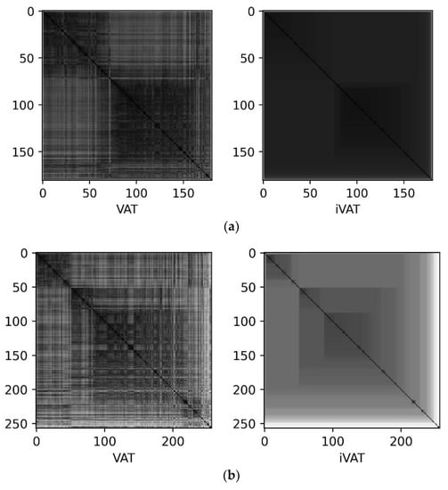
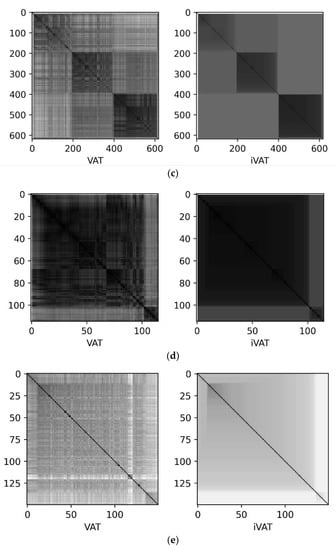
Figure 1.
Cluster heat maps. (a) Dataset 2P771A, containing 12 features. (b) Dataset 3D713V, containing 12 features. (c) Dataset 1526LE5, containing 120 features. (d) dataset GSE42568, containing 54,676 features. (e) Dataset GSE45827, containing 54,676 features.
6.1. The Transistors 2P771A Dataset
The use of the entire set of features in FCA leads to a huge number of concepts that make further analysis difficult. The work combines two approaches. Using the test theory algorithm, the smallest dead-end test (the support set of features) is found. FCA is then applied to the features of the dead-end test.
Application of the support set search algorithm (dead-end test) revealed four features sufficient to separate observations of different classes: T4, T6, T10, and T12.
For these features, the following boundary values were found:
T4 = 2.925;
T6 = 0.03425;
T10 = 0.6975;
T12 = 0.04065.
A computational experiment was carried out using two approaches:
- A concept formation algorithm, CloseByOne (FCA);
- A conceptual clustering algorithm, COBWEB.
The results obtained are presented in Appendix A and Figure A1 and Figure A2. It should be noted that class labels were used only to validate the results, but not to build sets of concepts. Figure A2 shows part of the formal concept lattice for 2P771A with a breakdown according to class (from CloseByOne).
When displaying the results, the following encoding of binary features was used in accordance with the cut-points:
1(+): x1 = 1, which corresponds to T4 ≥ 2.925;
1(−): x1 = 0, which corresponds to T4 < 2.925;
2(+): x2 = 1, which corresponds to T6 ≥ 0.03425;
2(−): x2 = 0, which corresponds to T6 < 0.03425;
…
As a result of the concept formation algorithm based on the selected features, 64 formal concepts were found. For each of them, an estimate was made using the normalized intracluster distance (D) and the silhouette index (S).
Examples of the most informative subgroups obtained by FCA are shown in Table 1.

Table 1.
Concepts obtained with FCA for the Transistors 2P771A dataset.
After imposing class labels, one can determine that among them there are pure-positive, pure-negative, and mixed concepts. The StandardQF score was used to evaluate compliance with known labels.
By analyzing the results obtained, the following conclusion can be drawn: If the silhouette index is high, say, more than 0.1, and the number of objects to be distinguished is large, for example, more than 20, then the distinguished subgroup is compact and at the same time corresponds to labels.
The study of the tree of concepts obtained with the help of Cobweb shows that the division into homogeneous subgroups (according to labels) occurs on the top branch. However, the description and interpretation of such concepts are difficult since they are based on the probabilities of accepting a certain value according to the features (Table 2).
Table 2.
Concepts obtained with COBWEB for the Transistors 2P771A dataset.
6.2. The Diodes 3D713V Dataset
The application of the algorithm for searching for the support set leads to the identification of five features sufficient to separate observations of different classes: T10, T2, T9, T8, and T11.
For these features, the following boundary values were found:
T10 = 0.4555;
T2 = 0.5275;
T9 = 0.3965;
T8 = 0.2035;
T11 = 0.6255.
The results obtained using the CloseByOne and COBWEB algorithms are shown in Appendix A and Figure A3 and Figure A4. For a more convenient presentation, the results are shown on a truncated set of the three most-influencing signs: T10, T2, and T9.
6.3. The Microcircuit 1526LE5 Dataset
The use of the support set search algorithm leads to the identification of seven cut-point values of features sufficient to separate observations of different classes:
T43 = −6.88;
T39 = 3.26;
T43 = −7.04;
T45 = −8.065;
T46 = −6.8;
T41 = 3.18;
T44 = −7.12.
The results obtained using the CloseByOne and COBWEB algorithms are presented in Appendix A, Figure A5 and Figure A6, and Table 3 and Table 4. For a more convenient presentation, the results are shown on a truncated set of the four most-influential feature cut-points.
Table 3.
Concepts obtained with CloseByOne for the Microcircuit 1526LE5 dataset.
Table 4.
Concepts obtained with COBWEB for the Microcircuit 1526LE5 dataset.
The analysis of the obtained results shows that with the help of both algorithms, subgroups containing objects of class a, as well as subgroups containing the union of objects of classes b and c, are distinguished. However, it is not possible to separate classes b and c using these algorithms, perhaps due to the similarity of these objects.
The features of data on industrial products (transistors, diodes, and microcircuits) should be noted. The data represent the results of the primary non-destructive tests to which all components are subjected. Further, for a part of the products, destructive tests are supposed to be carried out. However, the actual items in the kit can be produced under different production conditions. The results of destructive tests can only be extended to homogeneous products produced under similar conditions. The task is to identify homogeneous subgroups of products. Such allocation of subgroups should be justified and based on certain limits of parameter values, which can be considered as tougher norms for test parameters. To test the algorithms, sets of products were taken, which were formed by mixing several production batches. Batch-distribution information was used only to evaluate results and was not used to find concepts.
The logical concepts found with the help of FCA correspond to subgroups of products. These subgroups are described according to the above characteristics. Homogeneous subgroups, the elements of which belong mainly to the same batch, are distinguished via a low intracluster distance and a high value of the silhouette index (Figure A2, Figure A4 and Figure A6). At the same time, useful concepts can be located at different levels; that is, they can have different degrees (the number of literals). The concepts of the upper levels are more general and simple, the concepts of the lower levels are more selective (homogeneous) but have less coverage.
The result of the COBWEB algorithm is a lattice of probabilistic concepts. These concepts are fairly homogeneous already at the higher levels (for 2P771A transistors on the first branch and for 3D713V diodes on the second branch level). The branching factor is 2 or 3, and the branching depth is 3 and 4 for different data, i.e., the lattice of concepts turns out to be quite compact. The silhouette and intracluster distance values also make it possible to find homogeneous subgroups and, taking into account the coverage, select suitable concepts (Figure A1, Figure A3 and Figure A5). Neither FCA nor COBWEB could find subgroups corresponding to the second and third classes of 1526LE5 chips, possibly due to their indistinguishability according to the selected features.
6.4. The GSE42568 Dataset
For this dataset, one of the options for the support set of features consists of four binary features that correspond to the cut-point values:
206030_at = 6.079;
1553020_at = 4.346;
1555741_at = 4.236;
1553033_at = 3.993.
The results obtained using the CloseByOne and COBWEB algorithms are shown in Figure 2 and Figure 3. The color is responsible for label class.
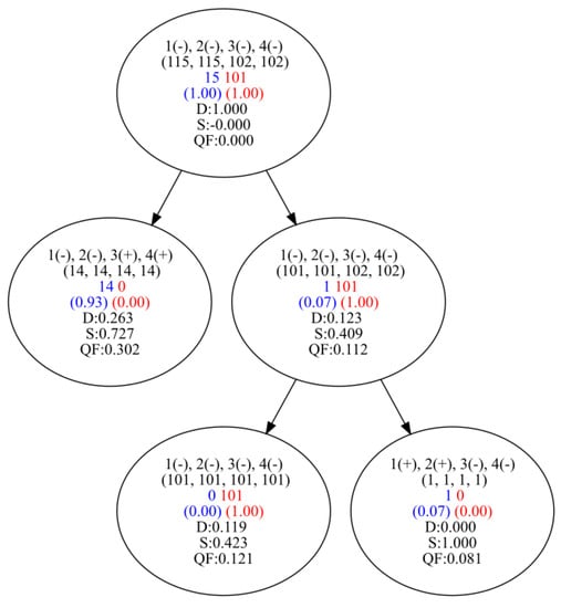
Figure 2.
Lattice of formal concepts for GSE42568 with distribution according to class (with COBWEB).
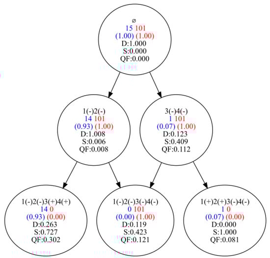
Figure 3.
Lattice of formal concepts for GSE42568 with distribution according to class (with CloseByOne).
6.5. The GSE45827 Dataset
The support set was used, consisting of six binary features that correspond to the cut-point values:
213007_at = 4.92074688046871;
221104_s_at = 3.51124853594935;
230595_at = 5.68936451280485;
235542_at = 5.43939791715374;
239071_at = 6.10825188641847;
239183_at = 3.24904004202841.
The results obtained using the CloseByOne and COBWEB algorithms are shown in Appendix A and Figure A7 and Figure A8.
Table 5.
Concepts obtained with CloseByOne for the GSE42568 and GSE45827 datasets.
Table 6.
Concepts obtained with COBWEB for the GSE42568 and GSE45827 datasets.
Data for the prediction of cancerous tumors according to gene expression are characterized by a rather large number of initial features; however, using the LAD methodology, a reference set of attributes of a small size was found. The data are characterized by a small number of examples that are not balanced across classes. The resulting grids of logical concepts and probabilistic concepts for the GSE42568 set are simple and easy to interpret (Figure 2 and Figure 3).
Examples of the GSE45827 set are also not balanced according to class (144 positive and 7 negative). However, using the FCA, we managed to find logical concepts that cover almost all positive observations (138 positive and no negative) as well as a concept that covers mostly negative observations (all 7 negative and 1 positive), which is characterized by the highest value of the silhouette among the concepts with a similar amount of coverage (Figure A8). With the help of COBWEB, it was possible to find a probabilistic concept, which includes only five negative examples along with one positive one (Figure A7).
Analyzing the obtained concept lattices (Figure 2, Figure 3, Figure A1, Figure A2, Figure A3, Figure A4, Figure A5 and Figure A6), it can be observed that the number of logical concepts obtained using FCA is greater than the number of concepts in the lattice constructed with COBWEB. However, it should be borne in mind that the FCA-based approach to identifying logical concepts can be formalized for subgroup sets, allowing for overlap between the subgroups. This does not apply to the lattice of concepts generated with COBWEB, wherein subgroup intersections are not allowed.
A graphical comparison of the running time of the CloseByOne and COBWEB algorithms is shown in Figure 4.
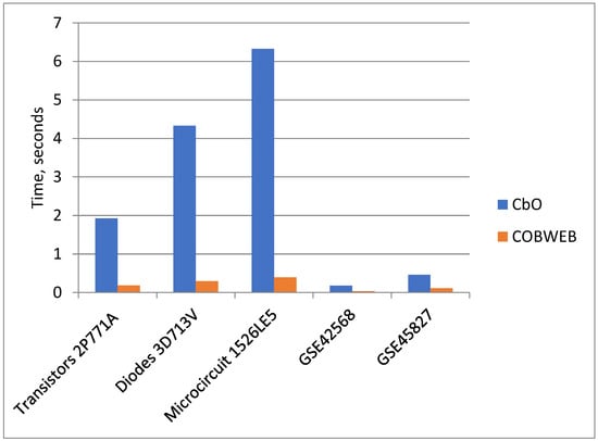
Figure 4.
A graphical comparison of the running time of the CloseByOne and COBWEB algorithms.
7. Discussion and Conclusions
FCA is most often used to analyze the classification of text data. In our work, we consider the use of FCA as an algorithm for identifying concepts in numerical data. This can be used both when searching for compact subgroups of objects in cluster analysis (unsupervised learning) and in classification problems to refine and justify the selected classes and search for new classes of objects in the data under study. For example, FCA can be used to identify subtypes of breast cancers based on the data on gene expression considered in this work. This line of work is the goal of further research.
The application of FCA for the described tasks requires an evaluation of the resulting concepts. According to the results of the work, we found that the most useful internal validation index for a concept as a compact subgroup is the silhouette index. Experiments show that a high value of the silhouette index (the specific cut-point value depends on the analyzed data) corresponds to the most informative subgroups (when compared with labels of previously known classes). Thus, when analyzing data with an unknown markup in advance, the silhouette index can be used as a selection criterion for concepts obtained in FCA to form compact subgroups of objects. It should be noted that these subgroups can intersect with each other, which corresponds to fuzzy clustering. The normalized intra-cluster distance can be used as an auxiliary criterion to confirm validation.
It is also worth noting that the concepts in FCA have a simple logical description, which is consistent with the principles of interpretive machine learning.
For comparison, the data were analyzed using the COBWEB conceptual clustering algorithm. This algorithm has significant differences from FCA both in the way of constructing a set of concepts and in the very type of concepts obtained. As a result of applying this algorithm, a hierarchy of concepts is formed, which corresponds to a clear clustering. At the same time, the concepts themselves are based on the probabilities of the values taken by the features. This makes it difficult to interpret the results and describe the concepts themselves in contrast to FCA, wherein only a part of the features can be used for a logical description. However, in general, these two algorithms give similar results in terms of the quality of the concepts they reveal.
To work with data described by a large number of features, it is proposed to supplement the algorithms with a search for a support set of features. The search for a support set is the basis of test theory. In our work, the search for a support set (support set) is carried out using a greedy algorithm that allows you to quickly find an approximate solution, the accuracy of which (in terms of the objective function of minimizing the number of features) is sufficient from a practical point of view. This approach successfully complements the FCA and COBWEB algorithms and allows them to be used to analyze data described by a large number of features and interpret the result.
An interesting topic for the further research is development of an algorithm for automatic selection of the set of the most informative logical concepts, which together cover the data examples.
Author Contributions
Conceptualization, I.M. and L.K.; methodology, I.M., N.R., and G.S.; software, N.R., S.M., and M.B.; validation, I.M., S.M., and G.S.; formal analysis, N.R. and G.S.; investigation, I.M., N.R., and G.S.; resources, I.M.; data curation, S.M. and G.S.; writing—original draft preparation, I.M. and M.B.; writing—review and editing, N.R., G.S., and L.K.; visualization, G.S. and N.R.; supervision, I.M. and L.K.; project administration, L.K.; funding acquisition, L.K. All authors have read and agreed to the published version of the manuscript.
Funding
This work was supported by the Ministry of Science and Higher Education of the Russian Federation (Grant No. 075-15-2022-1121).
Data Availability Statement
Data are available at https://www.ncbi.nlm.nih.gov and http://levk.info/data1526.zip (accessed on 21 April 2023).
Conflicts of Interest
The authors declare no conflict of interest.
Abbreviations
The following abbreviations are used in this manuscript:
| FCA | Formal Concept Analysis |
| LAD | Logical Analysis of Data |
| TT | Test Theory |
| CU | Category Utility |
| CbO | Close-by-One algorithm |
| QF | Quality Function |
Appendix A

Figure A1.
Part of lattice of formal concepts for 2P771A with distribution according to class (with COBWEB).
Figure A1.
Part of lattice of formal concepts for 2P771A with distribution according to class (with COBWEB).


Figure A2.
Part of lattice of formal concepts for 2P771A with distribution according to class (with CloseByOne).
Figure A2.
Part of lattice of formal concepts for 2P771A with distribution according to class (with CloseByOne).


Figure A3.
Lattice of formal concepts for 3D713V with distribution according to class (with COBWEB).
Figure A3.
Lattice of formal concepts for 3D713V with distribution according to class (with COBWEB).


Figure A4.
Part of lattice of formal concepts for 3D713V with distribution according to class (with CloseByOne).
Figure A4.
Part of lattice of formal concepts for 3D713V with distribution according to class (with CloseByOne).


Figure A5.
Lattice of formal concepts for 1526LE5 with distribution according to class (with COBWEB).
Figure A5.
Lattice of formal concepts for 1526LE5 with distribution according to class (with COBWEB).


Figure A6.
Lattice of formal concepts for 1526LE5 with distribution according to class (with CloseByOne).
Figure A6.
Lattice of formal concepts for 1526LE5 with distribution according to class (with CloseByOne).


Figure A7.
Lattice of formal concepts for GSE45827 with distribution according to class (with COBWEB).
Figure A7.
Lattice of formal concepts for GSE45827 with distribution according to class (with COBWEB).


Figure A8.
Part of lattice of formal concepts for GSE45827 with distribution according to class (with CloseByOne).
Figure A8.
Part of lattice of formal concepts for GSE45827 with distribution according to class (with CloseByOne).

References
- Dias, S.M.; Vieira, N.J. A methodology for analysis of concept lattice reduction. Inf. Sci. 2017, 396, 202–217. [Google Scholar] [CrossRef]
- Hammer, P.L. Partially defined boolean functions and cause-effect relationships. In Lecture at the International Conference on Multi-Attrubute Decision Making via OR-Based Expert Systems; University of Passau: Passau, Germany, 1986. [Google Scholar]
- Chikalov, I. Logical Analysis of Data: Theory, Methodology and Applications. In Three Approaches to Data Analysis. Intelligent Systems Reference Library, 41; Springer: Berlin/Heidelberg, Germany, 2013. [Google Scholar]
- Mortada, M.-A.; Carroll, T.; Yacout, S.; Lakis, A. Rogue components: Their effect and control using Logical Analysis of Data. J. Intell. Manuf. 2012, 23, 289–302. [Google Scholar] [CrossRef]
- Shaban, Y.; Yacout, S.; Balazinski, M. Tool wear monitoring and alarm system based on pattern recognition with Logical Analysis of Data. J. Manuf. Sci. Eng. 2015, 137, 041004. [Google Scholar] [CrossRef]
- Mortada, M.-A.; Yacout, S.; Lakis, A. Fault diagnosis in power transformers using multi-class Logical Analysis of Data. J. Intell. Manuf. 2014, 25, 1429–1439. [Google Scholar] [CrossRef]
- Ragab, A.; Ouali, M.-S.; Yacout, S.; Osman, H. Remaining useful life prediction using prognostic methodology based on Logical Analysis of Data and Kaplan-Meier estimation. J. Intell. Manuf. 2016, 27, 943–958. [Google Scholar] [CrossRef]
- Jocelyn, S.; Chinniah, Y.; Ouali, M.-S.; Yacout, S. Application of Logical Analysis of Data to machinery-related accident prevention based on scarce data. Reliab. Eng. Syst. Saf. 2017, 159, 223–236. [Google Scholar] [CrossRef]
- Dupuis, C.; Gamache, M.; Pagé, J.-F. Logical Analysis of Data for estimating passenger show rates at Air Canada. J. Air Transp. Manag. 2012, 18, 78–81. [Google Scholar] [CrossRef]
- Ragab, A.; de Carné de Carnavalet, X.; Yacout, S. Face recognition using multi-class Logical Analysis of Data. Pattern Recognit. Image Anal. 2017, 27, 276–288. [Google Scholar] [CrossRef]
- Kohli, R.; Krishnamurtib, R.; Jedidi, K. Subset-conjunctive rules for breast cancer diagnosis. Discret. Appl. Math. 2006, 154, 1100–1112. [Google Scholar] [CrossRef]
- Puszyński, K. Parallel implementation of Logical Analysis of Data (LAD) for discriminatory analysis of protein mass spectrometry data. Lect. Notes Comput. Sci. 2006, 3911, 1114–1121. [Google Scholar]
- Alexe, S.; Blackstone, E.; Hammer, P.L.; Ishwaran, H.; Lauer, M.S.; Pothier Snader, C.E. Coronary risk prediction by Logical Analysis of Data. Ann. Oper. Res. 2003, 119, 15–42. [Google Scholar] [CrossRef]
- Reddy, A.; Wang, H.; Yu, H.; Bonates, T.O.; Gulabani, V.; Azok, J.; Hoehn, G.; Hammer, P.L.; Baird, A.E.; Li, K.C. Logical Analysis of Data (LAD) model for the early diagnosis of acute ischemic stroke. BMC Med. Inform. Decis. Mak. 2008, 8, 30. [Google Scholar] [CrossRef]
- Kogan, A.; Lejeune, M.A. Combinatorial methods for constructing credit risk ratings. In Handbook of Financial Econometrics and Statistics; Lee, C.-F., Lee, J., Eds.; Springer: New York, NY, USA, 2014; pp. 439–483. [Google Scholar]
- Lejeune, M.A. Pattern-based modeling and solution of probabilistically constrained optimization problems. Oper. Res. 2012, 60, 1356–1372. [Google Scholar] [CrossRef]
- Wille, R. Restructuring lattice theory: An approach based on hierarchies of concepts. In Ordered Sets: Proceedings; Rival, I., Ed.; NATO Advanced Studies Institute, 83, Reidel: Dordrecht, The Netherlands, 1982; pp. 445–470. [Google Scholar]
- Ganter, B.; Wille, R. Formal concept analysis. In Mathematical Foundations; Springer: Berlin/Heidelberg, Germany, 1999. [Google Scholar]
- Tilley, T.; Eklund, P. Citation analysis using Formal Concept Analysis. In A Case Study in Software Engineering. In Database and Expert Systems Applications, DEXA’07, 18th International Workshop on; Springer: Berlin/Heidelberg, Germany, 2007; pp. 545–550. [Google Scholar]
- Cole, R.; Stumme, G. CEM—A Conceptual Email Manager. In Conceptual Structures: Logical, Linguistic, and Computational Issues. ICCS 2000. Lecture Notes in Computer Science; Ganter, B., Mineau, G.W., Eds.; Springer: Berlin/Heidelberg, Germany, 2000; Volume 1867. [Google Scholar]
- Poelmans, J.; Elzinga, P.; Neznanov, A.A.; Dedene, G.; Viaene, S.; Kuznetsov, S.O. Human-Centered Text Mining: A New Software System. In Advances in Data Mining. Applications and Theoretical Aspects. ICDM 2012. Lecture Notes in Computer Science; Perner, P., Ed.; Springer: Berlin/Heidelberg, Germany, 2012; Volume 7377. [Google Scholar]
- Belohlavek, R.; Sigmund, E.; Zacpal, J. Evaluation of IPAQ questionnaires supported by formal concept analysis. Inf. Sci. 2011, 181, 1774–1786. [Google Scholar] [CrossRef]
- Kaytoue, V.; Kuznetsov, S.O.; Napoli, A.; Duplessis, S. Mining gene expression data with pattern structures in formal concept analysis. Inf. Sci. 2011, 181, 1989–2001. [Google Scholar] [CrossRef]
- Amin, I.I.; Kassim, S.K. Applying formal concept analysis for visualizing DNA methylation status in breast cancer tumor subtypes. In Proceedings of the 2013 9th International Computer Engineering Conference (ICENCO), Giza, Egypt, 28–29 December 2013; IEEE: Piscataway, NJ, USA, 2013; pp. 37–42. [Google Scholar]
- Kuznetsov, S.O. Complexity of learning in concept lattices from positive and negative examples. Discret. Appl. Math. 2004, 142, 111–125. [Google Scholar] [CrossRef]
- Janostik, R.; Konecny, J.; Krajča, P. Interface between Logical Analysis of Data and Formal Concept Analysis. Eur. J. Oper. Res. 2020, 284, 792–800. [Google Scholar] [CrossRef]
- Alexe, G.; Alexe, S.; Hammer, P.; Vizvári, B. Pattern-based feature selection in genomics and proteomics. Ann. OR 2006, 148, 189–201. [Google Scholar] [CrossRef]
- Boros, E.; Hammer, P.; Ibaraki, T.; Kogan, A. Logical analysis of numerical data. Math. Program. 1997, 79, 163–190. [Google Scholar] [CrossRef]
- Shkaberina, G.; Rezova, N.; Tovbis, E.; Kazakovtsev, L. Visual Assessment of Cluster Tendency with Variations of Distance Measures. Algorithms 2023, 16, 5. [Google Scholar] [CrossRef]
- Lloyd, S.P. Least Squares Quantization in PCM. IEEE Trans. Inf. Theory 1982, 28, 129–137. [Google Scholar] [CrossRef]
- Michalski, R.S. Knowledge acquisition through conceptual clustering: A theoretical framework and an algorithm for partitioning data into conjunctive concepts. A special issue on knowledge acquisition and induction. Int. J. Policy Anal. Inf. Syst. 1980, 4, 219–244. [Google Scholar]
- Fonseca, N.A.; Santos-Costa, V.; Camacho, R. Conceptual clustering of multi-relational data. Proc. ILP 2012, 2011, 145–159. [Google Scholar]
- Fisher, D.H. Knowledge acquisition via incremental conceptual clustering. Mach. Learn. 1987, 2, 139–172. [Google Scholar] [CrossRef]
- Perner, P.; Attig, A. Fuzzy conceptual clustering. In Advances in Data Mining. Applications and Theoretical Aspects. ICDM 2010. Berlin, Germany, 12–14 July. Lecture Notes in Computer Science; Perner, P., Ed.; Springer: Berlin/Heidelberg, Germany, 2010; Volume 6171, pp. 71–85. [Google Scholar]
- Pons-Porrata, A.; Berlanga-Llavorí, R.; Ruiz-Shulcloper, J. Topic discovery based on text mining techniques. Inf. Process. Manag. 2007, 43, 752–768. [Google Scholar] [CrossRef]
- Pérez-Suárez, A.; Martínez-Trinidad, J.F.; Carrasco-Ochoa, J.A. A review of conceptual clustering algorithms. Artif. Intell. Rev. 2019, 52, 1267–1296. [Google Scholar] [CrossRef]
- Funes, A.; Ferri, C.; Hernández-Orallo, J.; Ramírez-Quintana, M.J. Hierarchical distance-based conceptual clustering. In Machine Learning and Knowledge Discovery in Databases. ECML PKDD 2008. Lecture Notes in Computer Science; Daelemans, W., Goethals, B., Morik, K., Eds.; Springer: Berlin/Heidelberg, Germany, 2008; Volume 5211, pp. 349–364. [Google Scholar]
- Chu, W.W.; Chiang, K.; Hsu, C.; Yau, H. An error-based conceptual clustering method for providing approximate query answers. Commun. ACM 1996, 39, 216. [Google Scholar] [CrossRef]
- Gutiérrez-Rodríguez, A.E.; Martínez Trinidad, J.F.; García-Borroto, M.; Carrasco-Ochoa, J.A. Mining patterns for clustering on numerical datasets using unsupervised decision trees. Knowl. Based Syst. 2015, 82, 70–79. [Google Scholar] [CrossRef]
- Romero-Zaliz, R.C.; Rubio-Escudero, C.; Perren-Cobb, J.; Herrera, F.; Cordón, O.; Zwir, I. A multiobjective evolutionary conceptual clustering methodology for gene annotation within structural databases: A case of study on the gene ontology database. IEEE Trans. Evol. Comput. 2008, 12, 679–701. [Google Scholar] [CrossRef]
- Fanizzi, N.; Amato, C.; Esposito, F. Evolutionary conceptual clustering of semantically annotated resources. In Proceedings of the International Conference on Semantic Computing 2007 (ICSC2007), Irvine, CA, USA, 17–19 September 2007; pp. 783–790. [Google Scholar]
- Segal, E.; Battle, A.; Koller, D. Decomposing gene expression into cellular processes. In Proceedings of the Pacific Symposium on Biocomputing, Kauai, HI, USA, 3–7 January 2003; pp. 89–100. [Google Scholar]
- Pei, J.; Zhang, X.; Cho, M.; Wang, H.; Yu, P.S. MaPle: A fast algorithm for maximal pattern-based clustering. In Proceedings of the Third IEEE International Conference on Data Mining 2003, ICDM 2003, Melbourne, FL, USA, 19–22 November 2003; pp. 259–266. [Google Scholar]
- Konecny, J.; Krajča, P. Systematic categorization and evaluation of CbO-based algorithms in FCA. Inf. Sci. 2021, 575, 265–288. [Google Scholar] [CrossRef]
- Kuznetsov, S.O. A fast algorithm for computing all intersections of objects from an arbitrary semilattice. Nauchno Tekhnicheskaya Inf. Seriya 2 Inf. Protsessy I Sist. 1993, 1, 17–20. [Google Scholar]
- Sivogolovko, E.; Novikov, B. Validating cluster structures in data mining tasks. In EDBT-ICDT’12; Association for Computing Machinery: New York, NY, USA, 2012; pp. 245–250. [Google Scholar]
- Golovanov, S.M.; Orlov, V.I.; Kazakovtsev, L.A. Recursive clustering algorithm based on silhouette criterion maximization for sorting semiconductor devices by homogeneous batches. IOP Conf. Ser. Mater. Sci. Eng. 2019, 537, 022035. [Google Scholar] [CrossRef]
- Lemmerich, F. Novel Techniques for Efficient and Effective Subgroup Discovery. Ph.D. Thesis, Bavarian Julius Maximilian University, Würzburg, Germany, 2014. [Google Scholar]
- Orlov, V.I.; Rozhnov, I.P.; Kazakovtsev, L.A.; Rezova, N.L.; Popov, V.P.; Mikhnev, D.L. Application of the K-Standards Algorithm for the Clustering Problem of Production Batches of Semiconductor Devices. In Proceedings of the 2021 XV International Scientific-Technical Conference on Actual Problems Of Electronic Instrument Engineering (APEIE), Novosibirsk, Russia, 19–21 November 2021; pp. 499–503. [Google Scholar]
- National Library of Medicine. Available online: https://www.ncbi.nlm.nih.gov/ (accessed on 10 March 2023).


Disclaimer/Publisher’s Note: The statements, opinions and data contained in all publications are solely those of the individual author(s) and contributor(s) and not of MDPI and/or the editor(s). MDPI and/or the editor(s) disclaim responsibility for any injury to people or property resulting from any ideas, methods, instructions or products referred to in the content. |
© 2023 by the authors. Licensee MDPI, Basel, Switzerland. This article is an open access article distributed under the terms and conditions of the Creative Commons Attribution (CC BY) license (https://creativecommons.org/licenses/by/4.0/).