Article

An Adaptive Deep Learning Neural Network Model to Enhance Machine-Learning-Based Classifiers for Intrusion Detection in Smart Grids

1
Department of Electrical and Electronic Engineering, Auckland University of Technology, Auckland 1010, New Zealand
2
College of Engineering, Qatar University, Doha P.O. Box 2713, Qatar
3
School of Electrical and Electronic Engineering, Nanyang Technological University, Singapore 639798, Singapore
*
Author to whom correspondence should be addressed.
Current address: Auckland University of Technology, Private Bag 92006, Auckland 1142, New Zealand.
These authors contributed equally to this work.
Algorithms 2023, 16(6), 288; https://doi.org/10.3390/a16060288
Submission received: 15 January 2023 / Revised: 28 May 2023 / Accepted: 30 May 2023 / Published: 2 June 2023

Abstract

:
Modern smart grids are built based on top of advanced computing and networking technologies, where condition monitoring relies on secure cyberphysical connectivity. Over the network infrastructure, transported data containing confidential information, must be protected as smart grids are vulnerable and subject to various cyberattacks. Various machine learning based classifiers were proposed for intrusion detection in smart grids. However, each of them has respective advantage and disadvantages. Aiming to improve the performance of existing machine learning based classifiers, this paper proposes an adaptive deep learning algorithm with a data pre-processing module, a neural network pre-training module and a classifier module, which work together classify intrusion data types using their high-dimensional data features. The proposed Adaptive Deep Learning (ADL) algorithm obtains the number of layers and the number of neurons per layer by determining the characteristic dimension of the network traffic. With transfer learning, the proposed ADL algorithm can extract the original data dimensions and obtain new abstract features. By combining deep learning models with traditional machine learning-based classification models, the performance of classification of network traffic data is significantly improved. By using the Network Security Laboratory-Knowledge Discovery in Databases (NSL-KDD) dataset, experimental results show that the proposed ADL algorithm improves the effectiveness of existing intrusion detection methods and reduces the training time, indicating a promising candidate to enhance network security in smart grids.

1. Introduction

Aiming to provide secure and dependable electrical services, the smart grid integrates power generation, transmission and distribution through digital communication technologies to detect and react to local changes in usage. The smart grid has two core subsystems: Advanced Metering Infrastructure (AMI) and Supervisory Control And Data Acquisition (SCADA), where AMI realises bi-directional data exchange between the electricity supplier and the customer to improve the efficiency of electricity consumption, while SCADA enables real-time monitoring and controlling of the transmission network [1]. However, due to the dependence among components in smart grid, a cyber attack could still lead to catastrophic failure of the entire grid [2]. Obviously, it is important to ensure the security of smart grid. In the National Institute of Standards and Technology Interagency Report (NISTIR) 7628, Guidelines for Smart Grid Cyber Security [3], information security in the smart grid consists of three essential elements: confidentiality (only authorised users can access the information), integrity (data must be accurate and consistent) and availability (information must be available with low-latency to authorized parties when needed). Therefore, smart grid should have self-healing and recovery capabilities to ensure communication and data security.
Cyber attacks on smart grid networks include control signal attacks, measurement attacks, and control-signal-measurement attacks [4]. Typical threats that impede data availability include flooding, route destruction, selective forwarding, wormhole, Byzantine attacks and denial-of-service (DoS) attacks. In general, security solutions can be divided into two main techniques, called prevention techniques and detection techniques. Prevention techniques aim to protect network data from being intercepted and encryption is usually adopted. Detection techniques aim to detect intruders [5], which include signature-based detection and anomaly-based detection. The former compares the observed attack patterns with known ones. The latter compares network traffic parameters with normal ones, where a change from normal traffic simply declares the presence of an intruder.
This paper presents an adaptive deep learning (ADL) neural network model to improve the recognition efficiency of anomalous attacks in smart grids. The proposed algorithm determines the number of layers and neurons per layer of the model, depending on the size of the smart grid. The contribution of this paper is threefold: Firstly, we propose an adaptive deep learning algorithm with a data pre-processing module, a neural network pre-training module and a classifier module, which work together classify intrusion data types using their high-dimensional data features. Secondly, the proposed ADL algorithm complements existing classification methods, and it can deployed with any existing feature classification algorithms to improve the classification performance. Finally, through experiments using the NSL-KDD dataset, we show that the robustness and flexibility of the proposed ADL algorithm. Altogether, by adding the proposed ADL algorithm, existing classifier algorithms can effectively discriminate between large ranges of network traffic, improve the accuracy of intrusion detection, converge faster, and reduce detection time significantly. The rest of the paper is organised as follows. Section 2 discusses the related work, while Section 3 presents the proposed ADL neural network model. Section 4 discusses the results, and Section 5 concludes the paper. For the sake of readability, Table 1 lists the abbreviations used in this paper.

2. Related Work

A smart grid consists of Home Area Network (HAN), Neighborhood Area Network (NAN) and Wide Area Network (WAN). The HAN consists of smart sensors, actuators and a user interface like home energy management system (HEMS). The NAN collects data from multiple HANs and transmits the data to the corresponding High Level Control Centres [6]. The NAN is therefore a dedicated channel for information exchange between the HAN and the WAN. Finally, the WAN connects multiple NANs, controlling the power transmission.
The Intrusion Detection System (IDS) monitors and detects malicious behaviour by collecting data information from key host nodes, building assessment models and analysing the network for the presence of illegal behaviour [7,8]. The IDS detects the attack trajectory of an attacked host and reports warnings to ensure the integrity of the network’s central host system. This will make the smart grid resistant to external network attacks [9].
Intrusion detection involves data acquisition, intrusion analysis and intrusion response. It reviews information from host logs, network segment protocol packets and gateways, and checks the network data using anomaly detection algorithms and discriminatory models [10]. The intrusion response module is used when anomalous attacks are reported by the intrusion analysis module. The module takes pre-defined measures, such as network disruption and alarm response, to prevent further deterioration of the situation.
Intrusion detection models are divided into host-based models, network-based models and feature-based models. Host-based models analyse the operating system’s audit trail and log messages of a single host [11]. They can detect viruses, malicious programs and destructive intrusion attacks on hosts [12]. However, the model monitors a host’s memory, which adversely affect the host’s performance. Additionally, its high memory space requirement does not support the handling of multiple attacks. For network-based models, they protect hosts by monitoring the number of network packets in a gateway to determine the network communication traffic of multiple hosts. This model can monitor large network sections with less memory [13]. However, the model cannot analyse the information flow of an encrypted network. It results in low detection accuracy in large-scale high-speed networks, thus it cannot handle fragmentation attacks. For feature-based detection model, it matches network intrusions to defined attack features through the misuse detection analysis system, which usually defines a separate feature for each anomalous event and uses a database to store the features for maintenance and matching [14]. This model enables efficient detection of correlated intrusion without generating excessive warning reports. However, this model requires constant updating of the feature database to maintain the system security, and it is unable to prevent malformed network attacks.
Intrusion detection methods include anomaly detection and misuse detection. The former is behavioural detection, which assumes that all network attacks are anomalous behaviour, then builds a model to differentiate normal behaviours from anomalous ones by comparison. Anomaly detection requires a simplified and accurate amount of features and reasonable threshold settings to ensure the optimal performance [15]. Anomaly detection can quickly detect network intrusions, but it requires heavy computation, leading to relatively high resource requirements. The latter monitors data at the gateway, compares the data signature with those in the database to determine if an intrusion is present [16]. However, it is impossible to locate the intrusion. Additionally, digital signatures are system dependent, making it difficult to standardise the detection procedure.
The KDD99 dataset was the data set used for The Third International Knowledge Discovery and Data Mining Tools Competition, which was held in conjunction with The Fifth International Conference on Knowledge Discovery and Data Mining (KDD-99). The KDD99 dataset is the most widely used dataset for intrusion detection. It consists of network data collected by Lincoln Laboratory over 69 days simulating the US Air Force LAN system with various types of network hosts and attacks [11]. The Network Security Laboratory - Knowledge Discovery in Databases (NSL-KDD) dataset is an improved version of the KDD99 dataset. It removes most of the duplicate data from the original KDD99 dataset. Each data entry in NSL-KDD contains 41-dimensional features and 1-dimensional label feature. Four types of feature data are available in the NSL-KDD, whose data label can indicate whether the data is normal data or not [12], with the data tag indicating the attack type.
The NSL-KDD data set includes four main parts, KDDTrain+, KDDTest+, KDDTrain+_ 20Percent and KDDTest-21 [17], where KDDTrain+ and KDDTest+ contain 125,973 and 22,543 data sets, espectively. The redundant part of the KDD99 data set is eliminated, KDDTrain+_20Percent provides an additional subset for training. In this dataset, network data is divided into five types: Normal, DoS attacks, user-to-root (U2R) attacks, root-to-local (R2L) attacks and Probe attacks. The normal type represents normal data; DoS attacks prevent the destination host from responding to external requests and cause a waste of resources; U2R attacks are user-unauthorised attacks, which attempt to gain root access; R2L attacks are login and access attacks by unauthorised hosts on the system; Probe attacks are port monitoring or port scanning. These five types include a total of 39 subtypes of attack types [18]. The specific classifications are shown in the Table 2.
In this paper, NSL-KDD dataset is used for the experiments. The dataset is first normalised to generate a standard dataset. With classical machine learning methods, a classifier is built for the standard dataset as a control group, and then the data features are extracted by the proposed ADL algorithm, and the generated data features are used to build a classifier to evaluate the effectiveness and usefulness of the proposed ADL algorithm.

2.1. Classification Algorithms

Intrusion detection scheme for smart grid based on machine learning refers to: converting the network intrusion problems into a packet type classification problems based on different intrusion types of packets, and using machine learning methods to train classification models to identify and classify intrusion packet types. However, due to the large number of network data features, if various features are used for training, it will increase the training time and model complexity, and the hardware requirements will also increase. To solve the problems of too many dimensions of network data features, there are various methods to extract data feature dimensions for reducing data feature dimensions. Consequently, intrusion detection can be treated as a packet type classification problem using machine learning. Feature extraction is usually adopted to reduce computation, whose common methods include correlation-based feature selection and encoding of data packets. The former uses a correlation function to select subsets of data, thereby reducing data size. The latter uses encoding to extract data features. Typical feature classification algorithms include K-nearest neighbour (KNN), Naïve Bayes (NB) classifier, Back Propagation Neural Network (BPNN) and Decision Tree (DT).
KNN Algorithm–The KNN algorithm first selects the value of K, which denotes the number of nearest neighbours. Between a given data point x and its neighbour y, their distance in the n-dimensional Euclidean space is
d x y = i = 1 n x i y i 2
Then it takes the K nearest neighbours as per the calculated Euclidean distance. Among these K neighbours, the algorithm counts the number of points in each class. Finally, it assigns x to that class for which the number of neighbours is maximum. The KNN algorithm is relatively accurate with simple implementation. Nevertheless, its efficiency will significantly decrease as the number of data points increases.
Naïve Bayes Algorithm—The Naïve Bayes classifier calculates conditional probability to perform classification.
y = arg max p y = C k p x | y = C k
With x = x 1 , x 2 , , x n , assuming that all features x are mutually independent, from Bayesian theorem we have
p C k p x | C k = p C k i = 1 n p x i | C k
Therefore, p C k | x p C k i = 1 n p x i | C k . With Laplace Smoothing, the prior probability is given by (where λ is the smoothing parameter)
p λ C k = i = 1 N I y i = C k + λ N + K λ
The conditional probability is calculated using
p λ x 1 = a j | y = C k = i = 1 N I x 1 = a j , y i = C k + λ i = 1 N I y i = C k + A λ
where K denotes the number of different values in y and A denotes the number of different values in a j . Usually λ = 1 .
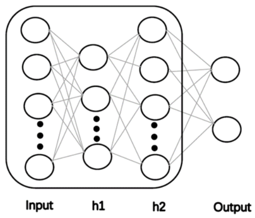
BPNN–The BPNN consists of an input layer, a hidden layer and an output layer. Given training set D = ( x 1 , y 1 ) , ( x 2 , y 2 ) , , ( x n , y n ) , x R d , y R I , as shown in Figure 1, for the j t h node (neuron), x 1 , x 2 , …, x i are the inputs of the neuron, which are connected by the weights of w j 1 , w j 2 , …, w j i to adjust the proportion of the input. Take the linear weighted sum as input and θ j as decision variable, hidden layer y j output is
y j = f i = 1 n w j i x i θ j
The parameters are set through the training data to obtain a parametric model of the prediction error, and the parameters are updated using the Gradient Descent method.
DT Algorithm–A DT consists of a root node, internal nodes and leaf nodes. The root node contains the entire data set. The internal nodes use different features to make category judgements and each leaf node represents the final judgement category. The complexity of the DT model is related to the number of layers of the tree. Under DT, information gain is the expected reduction in entropy of target variable Y for data sample S, due to sorting on variable A
G S , A = H A v V a l u e s ( A ) S v S H S v
Next, the impurity (e.g., data partition) of S is given by
G i n i S = 1 i = 1 K C i , S S 2

2.2. Feature Extraction Methods

Correlation-Based Feature Extraction–Correlation-based feature selection (CFS) uses the evaluation function to select a feature subset. For two continuous random variables X and Y, their linear correlation coefficient is given by
r X Y = i x i x i ¯ y i y i ¯ i x i x i ¯ 2 i y i y i ¯ 2
Automatic Encoder–Asymmetric Convolutional Encoder (ACE) can be used with a convolutional neural network [19] for unsupervised feature learning to extract the local features of the original data. The output of a hidden layer can be used as the input of the next layer. In each round of training operation of the convolutional layer, the algorithm first initialises k convolution sum, each convolution with weight w and bias b,
h k = f x w k + b k
The convolutional layer output from the upper layer is reconstructed (with bias c) to obtain the output data characteristics, which are adjusted by comparing the input and output data.
y = f k = 1 K h k w k + c k
This method uses multiple iterations of convolution, which increases the computational complexity.
Recently, intrusion detection was also studied for Internet of Things (IoT) and Jan et al. presented a lightweight intrusion detection method using supervised machine learning-based support vector machine (SVM) to detect malicious data injection [20]. However, it is difficult to apply it directly in smart grids due to different types of attacks. In [21], Karimipour et al. presented an unsupervised anomaly detection based on statistical correlation between measurements and time series partitioning to discover causal interactions between the subsystems. It adopted feature extraction utilising symbolic dynamic filtering (SDF) to reduce computational burden. In [22], Takiddin et al. presented an anomaly detector using stacked autoencoders with a long-short-term-memory (LSTM)-based sequence-to-sequence structure to detect electricity theft cyberattacks in smart grids. Inayat et al. presented an extensive survey on various cybersecurity enhancements of smart grids to detect false data injection attacks (FDIA), DoS attacks, distributed denial of service (DDoS) attacks, and spoofing attacks [23]. Interestingly, Zhou et al. presented a comprehensive survey for deep-learning-based abnormality detection in smart grids using multimodal image data [24], which include visible light, infrared, and optical satellite images. In [25], Berghout et al. reviewed different machine learning tools to detect cyberattacks in smart grids. In addition, it also highlighted various challenges, drawbacks and possible solutions of machine learning based cybersecurity applications in smart grids. A latest anomaly detection approach based on federated learning was proposed in [26], where machine learning models were trained locally in smart meters without sharing data with a central server, thus ensuring user Privacy. Table 3 compares our work with those machine learning based works found in the literature.

3. Proposed Adaptive Deep Learning

The proposed ADL algorithm consists of a data pre-processing module, a neural network pre-training module and a classifier module. In the data pre-processing module, the original dataset is normalised to generate a standard dataset. In the neural network pre-processing module, the algorithm is used to train the model and adjust the parameters to obtain a highly adaptive network model. The classifier module used high-dimensional data features to train a classifier to determine the intrusion data type on the test dataset.
With the proposed ADL algorithm, we extract data features through hidden layer neurons and change the distribution and structure of the data. The data features after each hidden layer are more accurate and essential. Transfer learning is embedded in the model so that it can be used for new tasks and improve the generalisation of the model. Next, deep belief networks (DBNs) enable compressed coding of raw data to accurately represent data features. A DBN consists of a multilayer Boltzmann machine network and a supervised back propagation network. The proposed algorithm combines DBNs to infer the appropriate number of hidden layers and the number of neurons per hidden layer for the neural network based on the original input data, allowing the pre-trained model to better match the size of the dataset and reduce the number of hidden layers. Too few hidden layers lead to under-reporting, while too many hidden layers lead to over-fitting. In the proposed ADL algorithm, parameters are used to control the training speed of the model and the accuracy of classification prediction. As shown in Figure 2, by adjusting the hidden layer, different data characteristics will be generated and transfer learning is adopted as shown in Figure 3.
As explained in Algorithm 1, by the proposed ADL algorithm, the number of hidden layers and the number of neurons are determined by the dimensionality of the original training data and the parameter θ , which balances training time, output accuracy and convergence speed. The range of θ is set from 0 to 1, with a step size of 0.1.
The ADL algorithm defines the number of neurons in each hidden layer of the deep neural network. The neurons before the output layer are the dimensions of the neurons in the highest layer. When θ is set close to 1, the feature dimension of the last hidden layer of the pre-trained model is close to that of the original data; when θ is set close to 0, the feature dimension of the last hidden layer of the pre-trained model is lower. The number of neurons in the first layer of the neural network is pre-set to be the same as the original data, and the data features are transformed through the hidden layers. The number of hidden layers and the number of neurons are determined by the original training data and θ . After the pre-training of the model, the back-propagation algorithm is used to adjust the parameters of the preset network model. The error gradient between the input training data v i and the model output data v i is adjusted, δ h is the weight of the node from the hidden layer to the next layer, and δ j is the error gradient of node j. The training results were obtained using the rectified linear activation function (ReLU), but experiments showed that the normal ReLU may result in the weights not being updated. Therefore, when x 0 , α x is used instead of 0 and the value of α is set to a smaller value to ensure that the weights can be updated correctly and speeds up the convergence of the network.
A x = α x , x 0 x , x > 0
The output layer uses a sigmoid function to fit the output, ranging from 0.1 to 1, which determines the behaviour and legitimacy of the data.
s x = 1 1 + e x
Algorithm 1 Proposed ADL algorithm: where v is number of training data samples, θ is the key parameter to balance the training speed and classification accuracy, η is the learning rate. N represents the set of neurons in the neural network; l is the number of neuron layers; D represents the dimension of the training data; and n i is the i t h neuron. δ k , δ h , W i j , and O i Δ W i j are the intermediate variables, W i j denotes the weights, and b j is the bias.
procedureADL( v , θ , η )               ▹ adaptive deep learning
     N t r a i n i n g _ d a t a v
    if  θ is empty then
         θ 0.3
    end if
    if  η is empty then
         η 0.1
    end if
     N
     D sizeof( N t r a i n i n g _ d a t a )
     l D D 5 5
     n i θ D
     i 2
    while  i l 1  do
         n i D D i 2 i 2 + θ D
         N . a p p e n d ( n i )
         i i + 1
    end while
     i 1
    while  i l  do
        use N to build the current layer and the n i neuron node
    end while
    output layer function s x 1 1 1 + e x 1 + e x
    for each training sample v i  do
        calculate the actual output of the model v i
    end for
     δ k v i 1 v i v i v i
     δ h v h 1 v h W h k δ k
     W i j W i j + Δ W i j
     O i Δ W i j W i j + η O i δ j
     b j δ b j
return x W + b
end procedure
After the model has been trained, the remaining part of the network other than the output layer is removed and the resultant model for the network is used for pre-processing. The number of neurons in the last layer of the hidden layers is the feature dimension of the output data. The algorithm determines the structure of the neural network through θ and the data dimension. The features of the data output from the hidden layers are considered as a downscaling of the original data. The smaller the dimension of the features generated by the model, the faster the detection, at the expense of reduced accuracy.
Four performance metrics are evaluated, namely accuracy, precision, recall, and F1-score. T P denotes the number of intrusion network data is correctly identified as intrusion network data. T N denotes the number of normal network data is correctly identified as normal network data. F P denotes the number of normal network data is incorrectly identified as intrusion network data. F N denotes the number of intrusion network data is wrongly identified as normal network data.
Accuracy is given by
s A = T P + T N T P + T N + F P + F N
Precision is given by
s P = T P T P + F P
Recall rate is given by
s R = T P T P + F N
F1-score is given by
s F 1 = 2 s P s R s P + s R

4. Results and Discussion

4.1. Preprocessing of Data

(a) IP Addresses and Port Numbers Removal—IP addresses and port numbers are removed from source and destination hosts because IP address and port numbers in the original dataset may lead to overtraining of neural networks and classifiers.
(b) Spaces Removal—Some tags in the dataset contain spaces that have no meaning in the actual data representation, but return different results in the data classification process, resulting in different classification of the packets. Thus, these spaces are removed.
(c) Label Encoding—The label of each piece of data is encoded. The label of each piece of data in the dataset contains the type of attack corresponding to that data, with different attack types corresponding to different specific strings. Encoding the strings into a specific value simplifies the learning process for the classifier. In the machine learning module, the classifier can learn the category values for each array.
(d) Data Normalisation—As the range of values taken from the data in the dataset does not meet the requirements of the classifier, the data range and format needs to be normalised to specify a minimum value for each data attribute. The normalisation and standardisation of the data provides a consistent value for the classifier, improving the correlation between the data and reducing the variability between the data features and improves the efficiency of the classifier.

4.2. Performance Evaluation

There are two types of classifiers considered in this paper–those based on four traditional machine learning models and those based on adaptive deep neural networks. As the training and test samples of the classifiers are the same, the interference of the data samples on the model results is effectively eliminated and the confidence of the comparison is improved.
80% of the data was used to train the proposed ADL model, while 80% of the remaining 20% data is used to train the classifier and 20% for testing. To verify the effectiveness of the ADL algorithm, we compare its performance with that of a traditional machine learning model for feature extraction. The experimental procedure uses the KNN, the DT, the NB algorithm and the BPNN to train the classifier. The raw data was passed through an adaptive deep neural network to obtain data features, which improved the classification accuracy of the classifier overall and also reduced the detection time of the network for abnormal data.

4.2.1. Two-Class Machine Learning Model

For the KNN algorithm, the value of K was set in the range of [3, 15] with a step size of 2. The average accuracy of the classifier with different parameters was tested. The experimental results show that the KNN algorithm produces better overall experimental results for the classifier, with the highest accuracy rates at K = 3 and K = 5 . Hereafter, we use K = 3 .
For the DT algorithm, the maximum depth of the tree and the minimum number of samples are needed for the leaf nodes. The range of values for depth is set to [10, 30] and the range of values for the minimum number of samples required by a leaf node is [2, 20]. First, the accuracy of classification of the DT algorithm at different depths was tested. Experimental results show that by the DT algorithm has the highest accuracy when the depth is 26 and the minimum number of leaf nodes is 2.
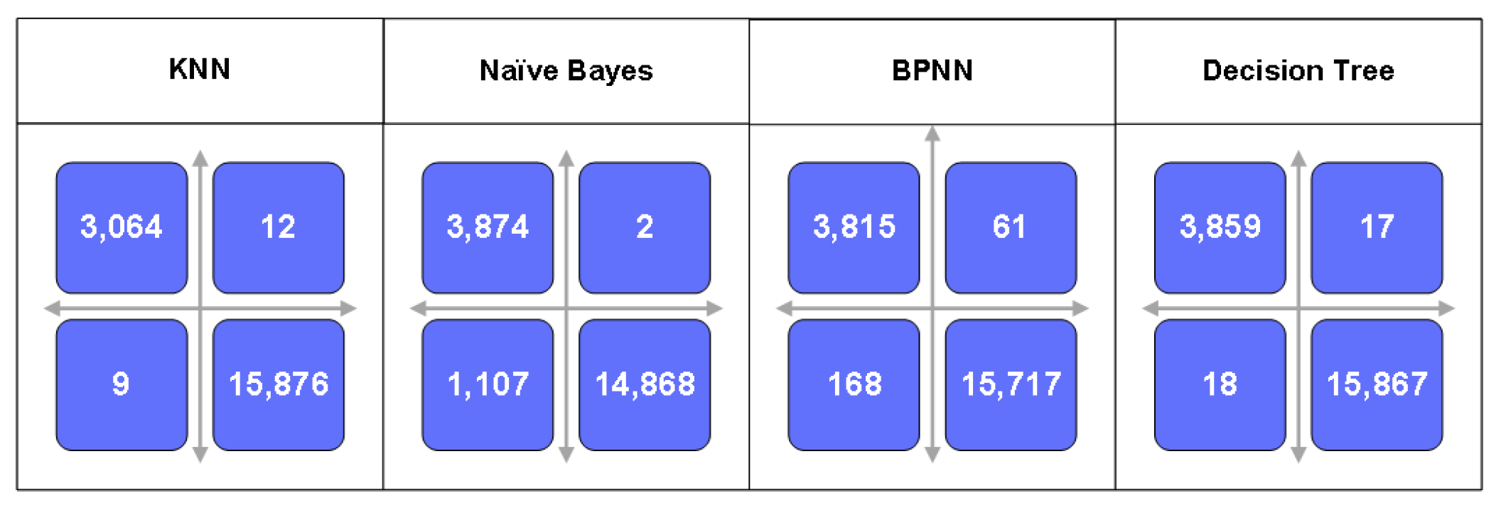
The confusion matrix is also known as the error matrix. It uses a matrix to visualize the performance of a machine learning algorithm. The column data of the confusion matrix represents the predicted values, while the row data represents the actual values. The confusion matrix is introduced to indicate whether there is confusion between different categories, i.e. whether there is a misclassification. The results of the confusion matrix produced by different algorithms are shown in Figure 4. The X-axis represents the predicted values and the Y-axis represents the true values. The values in the first quadrant represent data where the predicted value is an attack and the true value is normal. The values in the second quadrant represent data where the predicted value is normal and the true value is normal. Values in the third quadrant represent data where the predicted value is normal and the true value is an attack. A value in the fourth quadrant represents data for which the predicted value is an attack and the true value is an attack. From Figure 4, we can see that KNN outperforms other three classification techinques, followed by DT and BPNN. The performance of Naïve Bayes is the worst in terms of two-class classification.
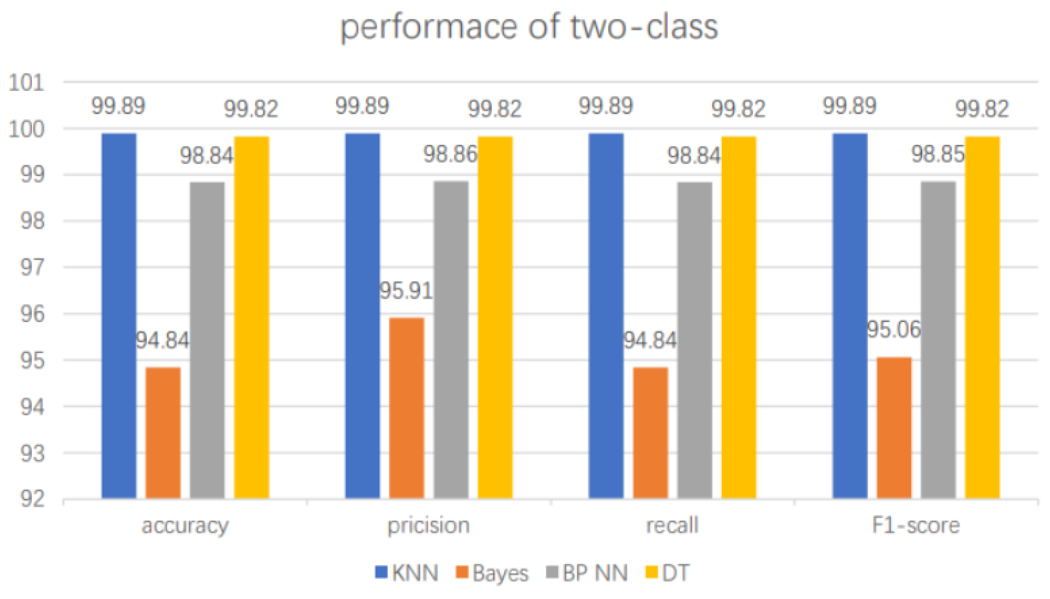
The experimental results are shown in Figure 5. Results show that with two classifications, all packets were divided into two categories–abnormal data and normal data. The abnormal data was not further classified and the sample imbalance was relatively less of a problem. However, in practical applications, the categories of abnormal data need to be further divided, so the effect of sample imbalance on the training results should be considered in the subsequent multi-classification cases.

4.2.2. Multi-Class Machine Learning Model

In the same process as for the two classifications, dataset machine learning models were used for training and testing. In order to more accurately simulate network attacks in real life situations and to classify different attacks. This paper extends the two classifications into multiple classifications to identify different types of attacks.
(1) KNN algorithm parameter setting: In order to save computational effort and processing time, the range and step size of K values were set to be the same as in the case of two classification. The experimental results show that the highest classification accuracy is achieved with K = 3. The value of K is set in line with the case of two classification, which reduces the complexity of the comparison and the difficulty of the calculation to some extent.
(2) Decision Tree algorithm parameter setting: As in the case of two classification, the algorithm needs to determine the maximum depth and minimum number of samples required for the leaf nodes in the multi-level classification case. The range of values and step size of each parameter are set to the same as in the two classification case.
The experimental results showed that the classification accuracy was stable at 99.84% when the maximum depth of the tree was greater than or equal to 27. To reduce the computational effort and the complexity of machine learning as much as possible, the maximum depth of the tree was set to 27. Subsequently, the number of leaves and he minimum number of samples of nodes was tested. The experimental results showed that when the depth of the Decision Tree is 27, the classification accuracy of the classifier decreases as the minimum number of samples of the leaf nodes increases. So the maximum number of samples of the leaf nodes was set to 2.
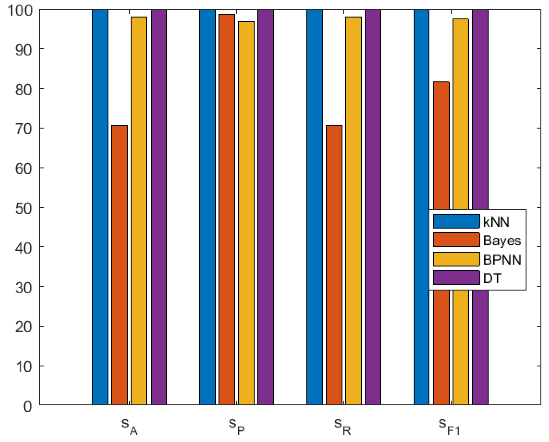
For the KNN algorithm, K = 3 provides the best results. For the DT algorithms, result show that optimal results are achieved when the maximum depth of the tree is 27 and the maximum number of samples of the leaf nodes is 2. Figure 6 shows the confusion matrix for multi-class classification by KNN, Naive Bayes, BPNN and DT. Figure 7 shows the results for multiple classifications.
After 10 experiments comparing the s F 1 of the ADL neural network model and the traditional machine learning classification model, it was demonstrated that the classification performance of the ADL neural network model was better. Since the s F 1 refers to the weighted average of precision and recall, it can be concluded experimentally that the s F 1 of the ADL classifier reaches its highest value when θ = 0.8. By applying the ADL algorithm with the traditional machine learning algorithm, the performance metrics of the classifier were significantly improved. In particular, the s A of the NB algorithm improved from 94.84% to 98.77% and the s R improved from 95.06% to 99.75%. The improvements in accuracy and recall were more pronounced than those model without the ADL algorithm to extract features. The performance metrics are summarised in Table 4.
In traditional machine learning, the NB algorithm has the worst performance, whose performance is summarised in Table 5. Next, after adding the ADL algorithm to the NB algorithm, Table 6 shows the effect of using the ADL algorithm on the performance improvement of the NB algorithm. The reason for the negligible performance improvement for the DoS data is that the main attacks in the network come from DoS attacks, so the number of DoS attacks is large and better classification can be achieved without feature extraction. R2L and U2R are relatively small data in the dataset and the performance is greatly improved after feature extraction. The S A of R2L is improved from 84.13% to 91.32%, the S P increased from 91.23% to 96.44%, the S A of U2R increased from 28.49% to 43.83%, and the S P increased from 66.88% to 75.02%.
To investigate the effect of ADL algorithm on the classifier performance at different θ values, parametric analysis of θ was carried out on selected datasets. The output efficiency of the model was determined by comparing the accuracy of the classifier at different values of θ . From the experimental results, θ can affect the accuracy of the classifier by adjusting the dimensionality of feature extraction. When θ was set to [0.1, 0.5], the S A of the ADL algorithm improved gracefully. When θ > 0.6 , the S A of the ADL algorithm is saturated and the stability of the ADL algorithm is high.
Through experiements using the NSL-KDD dataset, the performance of the naïve Bayesian algorithm classifier is greatly improved after processing by the ADL algorithm (see Table 6). The reason for the smaller performance improvement for the DoS data is that the main attacks in the network environment come from Dos attacks, so the number of Dos attacks is larger and better classification can be achieved without feature extraction. R2L and U2L are relatively small data in the dataset and the performance is greatly improved after feature extraction. The accuracy of R2L is improved from 84.13% to 91.32%, the accuracy rate increased from 91.23% to 96.44%, the accuracy rate of U2L increased from 28.49% to 43.83%, and the accuracy rate increased from 66.88% to 75.02%.
Based on the CFS method, the data features of the subset are extracted using specific measurement indicators, the correlation matrices of different feature subsets are established, and the function values of the subset matrices are solved to select the best correlation feature matrix A subset. The results of CFS are shown in Table 7. Next, coding-based feature extraction methods often use ACE for feature extraction. Thus, for the sake of comparison, we also present results of ACE in Table 8.
The experimental results show that the proposed ADL algorithm together with the NB algorithm (see Table 6) has a greater improvement in the classification accuracy of R2L and U2R compared to the ACE algorithm, and the overall performance of the algorithm is also better. This indicates that the algorithm is more efficient in intrusion detection for small sample data. Also, the use of encoders is avoided, as is the possibility of increased computational complexity. However, the s F 1 of the ADL algorithm is relatively low and could be improved in future work.
Results showed that the classification accuracy of the ADL algorithm increased as θ increased in [0.1, 0.5]. The accuracy tends to saturate when θ is greater than 0.6, demonstrating the stability and feasibility of the proposed ADL algorithm. Meanwhile, comparison results proved that the ADL algorithm is better than the CFS feature extraction algorithm when the amount of sample data is large. Compared with the ACE feature extraction algorithm, the ADL algorithm improves the classification accuracy of R2L and U2R.

5. Conclusions

This paper proposes an adaptive deep learning algorithm that determines the number of hidden layers and neurons of a neural network by extracting the dimension of the original data. By setting parameters to balance the detection time and output accuracy, the proposed ADL algorithm can adapt to different network environments and network sizes. Moreover, by combining the ADL algorithm with traditional machine learning algorithms, they can effectively discriminate between large ranges of network traffic, improve the accuracy of intrusion detection, converge faster, and reduce detection time significantly. In particular, Naïve Bayes classification produces the worst performance as compared to KNN, DT and BPNN. After adding the proposed ADL to Naïve Bayes classification, its performance can be improved significantly. For example, the accuracy of R2L is improved from 84.13% to 91.32%, the accuracy rate increased from 91.23% to 96.44%, the accuracy rate of U2L increased from 28.49% to 43.83%, and the accuracy rate increased from 66.88% to 75.02%. The proposed ADL algorithm can also improve the performance of the other three traditional classifiers to different extent. For future work, a real-time packet capture platform can be adopted for analysis and further optimisation of the proposed ADL algorithm.
For future work, a real-time packet capture platform can be set up for further analysis and optimisation of the proposed ADL algorithm. In particular, the experiment utilised a combination of deep neural networks and traditional machine learning algorithms, with specific parameters set for different network sizes to reduce the training time of the network. However, the current process of parameter learning is resource-intensive in terms of computational power and computational time, and future research could optimise the learning time of parameters and the requirement for hardware computational power. In addition, to study the complex data patterns and low footprint stealth attacks of the contemporary network traffic, we plan to verify the performance of our proposed ADL algorithm using the UNSW-NB15 dataset [27].

Author Contributions

Conceptualization, X.J.L. and M.M.; methodology, M.M.; software, Y.S. and M.M.; validation, Y.S., M.M. and X.J.L.; formal analysis, Y.S., M.M. and X.J.L.; writing—original draft preparation, X.J.L.; writing—review and editing, X.J.L. and M.M.; supervision, M.M. All authors have read and agreed to the published version of the manuscript.

Funding

This research received no external funding.

Data Availability Statement

Not applicable.

Conflicts of Interest

The authors declare no conflict of interest.

References

  1. Zhang, Y.; Wang, L.; Xiang, Y. Power System Reliability Analysis With Intrusion Tolerance in SCADA Systems. IEEE Trans. Smart Grid 2016, 7, 669–683. [Google Scholar] [CrossRef]
  2. Nguyen, T.N.; Liu, B.-H.; Nguyen, N.P.; Chou, J.-T. Cyber Security of Smart Grid: Attacks and Defenses. In Proceedings of the ICC 2020—2020 IEEE International Conference on Communications (ICC), Dublin, Ireland, 7–11 June 2020. [Google Scholar]
  3. Harvey, M.; Long, D.; Reinhard, K. Visualizing NISTIR 7628, Guidelines for Smart Grid Cyber Security. In Proceedings of the 2014 Power and Energy Conference at Illinois (PECI), Champaign, IL, USA, 28 February–1 March 2014; pp. 1–8. [Google Scholar]
  4. Zhang, H.; Liu, B.; Wu, H. Smart Grid Cyber-Physical Attack and Defense: A Review. IEEE Access 2021, 9, 29641–29659. [Google Scholar] [CrossRef]
  5. Khan, S.; Kifayat, K.; Bashir, A.K.; Gurtov, A.; Hassan, M. Intelligent intrusion detection system in smart grid using computational intelligence and machine learning. Trans. Emerg. Telecommun. Technol. 2021, 32, e4062. [Google Scholar] [CrossRef]
  6. Meng, W.; Ma, R.; Chen, H.-H. Smart grid neighborhood area networks: A survey. IEEE Netw. 2014, 28, 24–32. [Google Scholar] [CrossRef]
  7. Khoei, T.T.; Slimane, H.O.; Kaabouch, N. A Comprehensive Survey on the Cyber-Security of Smart Grids: Cyber-Attacks, Detection, Countermeasure Techniques, and Future Directions. arXiv 2022, arXiv:2207.07738. [Google Scholar]
  8. Ding, J.; Qammar, A.; Zhang, Z.; Karim, A.; Ning, H. Cyber Threats to Smart Grids: Review, Taxonomy, Potential Solutions, and Future Directions. Energies 2022, 15, 6799. [Google Scholar] [CrossRef]
  9. Vaidya, B.; Makrakis, D.; Mouftah, H.T. Device authentication mechanism for Smart Energy Home Area Networks. In Proceedings of the 2011 IEEE International Conference on Consumer Electronics (ICCE), Las Vegas, NV, USA, 9–12 January 2011; pp. 787–788. [Google Scholar]
  10. Bae, H.-S.; Lee, H.-J.; Lee, S.-G. Voice recognition based on adaptive MFCC and deep learning. In Proceedings of the 2016 IEEE 11th Conference on Industrial Electronics and Applications (ICIEA), Hefei, China, 5–7 June 2016; pp. 1542–1546. [Google Scholar]
  11. Nicanfar, H.; Jokar, P.; Beznosov, K.; Leung, V.C.M. Efficient Authentication and Key Management Mechanisms for Smart Grid Communications. IEEE Syst. J. 2014, 8, 629–640. [Google Scholar] [CrossRef]
  12. Hao, J.; Kang, E.; Sun, J.; Wang, Z.; Meng, Z.; Li, X.; Ming, Z. An Adaptive Markov Strategy for Defending Smart Grid False Data Injection From Malicious Attackers. IEEE Trans. Smart Grid 2018, 9, 2398–2408. [Google Scholar] [CrossRef]
  13. Cui, J.; Long, J.; Min, E.; Mao, Y. WEDL-NIDS: Improving network intrusion detection using word embedding-based deep learning method. In MDAI 2018: Modeling Decisions for Artificial Intelligence; Springer: Berlin/Heidelberg, Germany, 2018; pp. 283–295. [Google Scholar]
  14. Song, C.; Sun, Y.; Han, G.; Rodrigues, J.J.P.C. Intrusion detection based on hybrid classifiers for smart grid. Comput. Electr. Eng. 2021, 93, 107212. [Google Scholar] [CrossRef]
  15. Hu, H.; Doufexi, A.; Armour, S.; Kaleshi, D. A Reliable Hybrid Wireless Network Architecture for Smart Grid Neighbourhood Area Networks. In Proceedings of the 2017 IEEE Wireless Communications and Networking Conference (WCNC), San Francisco, CA, USA, 19–22 March 2017; pp. 1–6. [Google Scholar]
  16. Gobena, Y.; Durai, A.; Birkner, M.; Pothamsetty, V.; Varakantam, V. Practical architecture considerations for Smart Grid WAN network. In Proceedings of the 2011 IEEE/PES Power Systems Conference and Exposition, Phoenix, AZ, USA, 20–23 March 2011; pp. 1–6. [Google Scholar]
  17. Mohi-ud-din, G. “NSL-KDD”, IEEE Dataport, Published by IEEE, USA. Available online: https://dx.doi.org/10.21227/425a-3e55 (accessed on 29 December 2018).
  18. Shone, N.; Ngoc, T.N.; Phai, V.D.; Shi, Q. A Deep Learning Approach to Network Intrusion Detection. IEEE Trans. Emerg. Top. Comput. Intell. 2018, 2, 41–50. [Google Scholar] [CrossRef] [Green Version]
  19. Dong, S.; Wang, P.; Abbas, K. A survey on deep learning and its applications. Comput. Sci. Rev. 2022, 40, 100379. [Google Scholar] [CrossRef]
  20. Jan, S.U.; Ahmed, S.; Shakhov, V.; Koo, I. Toward a Lightweight Intrusion Detection System for the Internet of Things. IEEE Access 2019, 7, 42450–42471. [Google Scholar] [CrossRef]
  21. Karimipour, H.; Dehghantanha, A.; Parizi, R.M.; Choo, K.-K.R.; Leung, H. A Deep and Scalable Unsupervised Machine Learning System for Cyber-Attack Detection in Large-Scale Smart Grids. IEEE Access. 2019, 7, 80778–80788. [Google Scholar] [CrossRef]
  22. Takiddin, A.; Ismail, M.; Zafar, U.; Serpedin, E. Deep Autoencoder-Based Anomaly Detection of Electricity Theft Cyberattacks in Smart Grids. IEEE Syst. J. 2022, 16, 4106–4117. [Google Scholar] [CrossRef]
  23. Inayat, U.; Zia, M.F.; Mahmood, S.; Berghout, T.; Benbouzid, M. Cybersecurity Enhancement of Smart Grid: Attacks, Methods, and Prospects. Electronics 2022, 11, 3854. [Google Scholar] [CrossRef]
  24. Zhou, F.; Wen, G.; Ma, Y.; Geng, H.; Huang, R.; Pei, L.; Yu, W.; Chu, L.; Qiu, R. A Comprehensive Survey for Deep-Learning-Based Abnormality Detection in Smart Grids with Multimodal Image Data. Appl. Sci. 2022, 12, 5336. [Google Scholar] [CrossRef]
  25. Berghout, T.; Benbouzid, M.; Muyeen, S.M. Machine learning for cybersecurity in smart grids: A comprehensive review-based study on methods, solutions, and prospects. Int. J. Crit. Infrastruct. Prot. 2022, 38, 100547. [Google Scholar] [CrossRef]
  26. Jithish, J.; Alangot, B.; Mahalingam, N.; Yeo, K.S. Distributed Anomaly Detection in Smart Grids: A Federated Learning-Based Approach. IEEE Access 2023, 11, 7157–7179. [Google Scholar] [CrossRef]
  27. Moustafa, N.; Slay, J. UNSW-NB15: A comprehensive data set for network intrusion detection systems (UNSW-NB15 network data set). In Proceedings of the 2015 Military Communications and Information Systems Conference (MilCIS), Canberra, Australia, 10–12 November 2015; pp. 1–6. [Google Scholar]
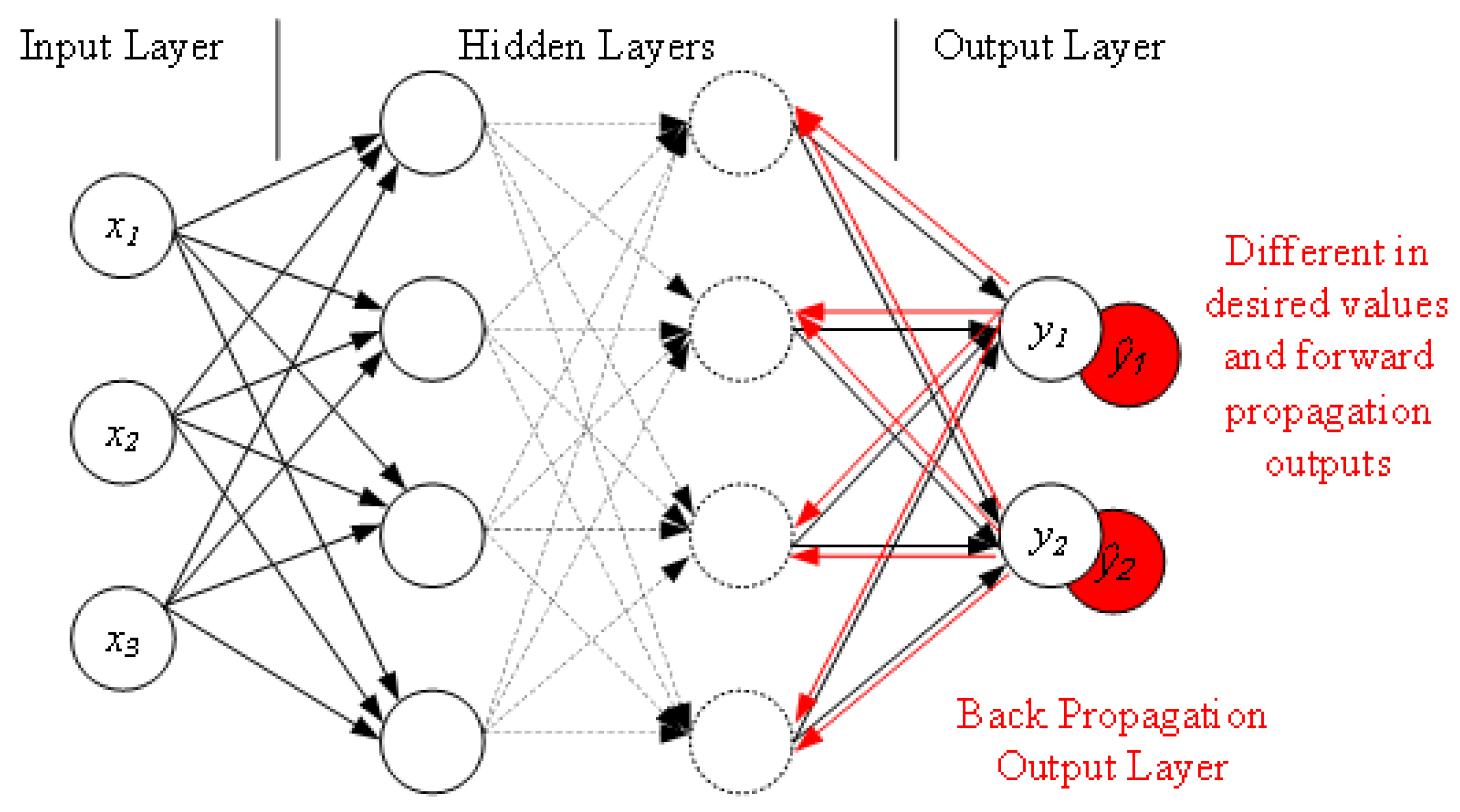
Figure 1. Illustration diagram shows how a Back Propagation Neural Network works.
Algorithms 16 00288 g001
Figure 2. Illustration diagram of the adaptive deep learning framework.
Algorithms 16 00288 g002
Figure 3. Illustration diagram of the model of transferring learning.
Algorithms 16 00288 g003
Figure 4. The confusion matrix results of two-class classification using the existing four classification methods: KNN, Naïve Bayes, BPNN and DT.
Algorithms 16 00288 g004
Figure 5. Performance comparison of two-class classifications using the existing four classification methods: KNN, Naïve Bayes, BPNN and DT.
Algorithms 16 00288 g005
Figure 6. The confusion matrix results of multi-classification using the existing four classification methods: KNN, Naïve Bayes, BPNN and DT.
Algorithms 16 00288 g006
Figure 7. Performance comparison of multi-classification using the existing four classification methods: KNN, Naïve Bayes, BPNN and DT.
Algorithms 16 00288 g007
Table 1. Nomenclature.
AbbreviationTerm
ACEasymmetric convolutional encoder
ADLAdaptive deep learning
AMIAdvanced Metering Infrastructure
BPNNBack Propagation Neural Network
CFScorrelation-based feature selection
DBNdeep belief network
DDoSdistributed denial of service
DoSdenial-of-service
DTDecision Tree
FDIAfalse data injection attacks
HANHome Area Network
HEMShome energy management system
IDSIntrusion Detection System
IoTInternet of Things
KDDKnowledge Discovery in Databases
KNNK-nearest neighbour
LSTMlong-short-term-memory
NISTIRNational Institute of Standards and Technology Interagency Report
NSL-KDDNetwork Security Laboratory - Knowledge Discovery in Databases
R2Lroot-to-local
ReLUrectified linear activation function
SCADASupervisory Control And Data Acquisition
SDFsymbolic dynamic filtering
SVMSupport Vector Machine
U2Ruser-to-root
WANWide Area Network
Table 2. Summary of attacks types labeled in the NSL-KDD dataset.
TypeAttackDescription
NormalNormal data trafficNormal data type
DoSBack, Land, Neptune,
Pod, Smurf, Teardrop,
Mailbomb, Processtable,
UDPstorm, Apache2, Worm
Denial of service attacks,
which make computers and
networks unable to provide
normal services
ProbeSatan, Nmap, Mscan, Saint,
IP sweep, Portsweep
Port attack, scan port
vulnerabilities to attack
U2RBuffer overflow, Sql attack,
XtermLoadmodule, Rootkit,
Perl, Ps
Unauthorized users obtain
root vulnerabilities through
network vulnerabilities and
perform illegal operations
R2LGuess password, Imap,
Multihop, Ftp write, Phf,
Warezmaster, Xclock,
Xsnoop, Snmpguess,
Snmpgetattack, Sendmail,
Httptunnel, Named
Remote attack, users remotely
log in operate illegally
through accounts and
passwords
Table 3. Comparison of machine learning based intrusion detection techniques.
WorksLearning TypeKey TechniquesDatasets
[5]SupervisedParticle swarm optimisation
based neural network
KDD99 and NSL-KDD
[13]SupervisedWork embedding-based
deep learning
Intrusion Detection
Evaluation Dataset
(ISCX2012)
[14]Semi-supervisedLong short-term memory and
extreme gradient boosting with
genetic algorithm
NSL-KDD
[18]UnsupervisedNonsymmetric deep
autoencoder
KDD99 and NSL-KDD
[20]SupervisedSupport vector machineIntrusion Detection
Evaluation Dataset
(CIC-IDS2017)
[21]UnsupervisedFeature extraction using
symbolic dynamic filtering
Data from testbed
from Matpower
[22]SupervisedLong short-term memory
with stacked autoencoders
State Grid Corporation
of China Dataset
[26]SupervisedFederated LearningKDD99, NSL-KDD and
CIDDS-001 datasets
This workSupervisedAdaptive deep learning
using deep belief network
NSL-KDD
Table 4. Performance comparison of existing classifiers with and without the proposed adaptive deep learning algorithm.
Model s A (%) s P (%) s R (%) S F 1 (%)
kNN99.8999.8999.8999.89
kNN with ADL99.2399.4998.7499.15
Decision Tree99.8299.8299.8299.82
DT with ADL99.5899.7299.5899.65
Bayes94.8495.9194.8495.06
Bayes with ADL98.7795.2599.7597.70
BPNN98.8498.8698.8498.05
BPNN with ADL99.1599.3699.8299.13
Table 5. Results using Naïve Bayes classifier.
Data Type s A (%) s P (%) s R (%) S F 1 (%)
Normal99.2498.8699.4399.81
DoS99.8599.8698.8599.85
Probe95.6497.4295.4396.41
R2L84.1391.2383.2387.07
U2R28.4966.8828.5740.02
Table 6. Results using Naïve Bayes classifier together with the proposed ADL Algorithm.
Data Type s A (%) s P (%) s R (%) S F 1 (%)
Normal99.9198.6599.9099.78
DoS99.8599.8898.8599.87
Probe98.8399.7599.8799.34
R2L91.3296.4490.3993.31
U2R42.8375.0242.8554.45
Table 7. Results using the Correlation Feature Selection Algorithm.
Data Type s A (%) s P (%) s R (%) S F 1 (%)
Normal99.5810097.283.9
DoS99.7697.599.389.7
Probe99.8184.799.791.6
R2L24.3655.699.790.3
U2R60.1782.399.772.08
Table 8. Results using the Asymmetric Convolutional Encoder algorithm.
Data Type s A (%) s P (%) s R (%) S F 1 (%)
Normal99.5810099.6499.82
DoS99.7610099.8199.90
Probe99.8110099.3296.61
R2L24.3610088.3693.83
U2R10.1741.3247.2344.08
Disclaimer/Publisher’s Note: The statements, opinions and data contained in all publications are solely those of the individual author(s) and contributor(s) and not of MDPI and/or the editor(s). MDPI and/or the editor(s) disclaim responsibility for any injury to people or property resulting from any ideas, methods, instructions or products referred to in the content.