Rotating Machinery Fault Detection Using Support Vector Machine via Feature Ranking

Abstract

Artificial intelligence has succeeded in many different areas in recent years. Especially the use of machine learning algorithms has been very popular in all areas, including fault detection. This paper explores a case study of applying machine learning techniques and neural networks to detect ten different machinery fault conditions using publicly available data sets collected from a tachometer, two accelerometers, and a microphone. Ten different conditions were classified using machine learning algorithms. Fifty-eight different features are extracted from time and frequency by applying the Short-Time Fourier Transform to the data with the window size of 1000 samples with 50% overlap. The Support Vector Machine models provided fault classification with 99.8% accuracy using all fifty-eight features. The proposed study explores the dimensionality reduction of the extracted features. Fifty-eight features were ranked using the Decision Tree model to identify the essential features as the classifier predictors. Based on feature extraction and raking, eleven predictors were extracted leading to reduced training complexity, while achieving a high classification accuracy of 99.7% could be obtained in less than half of the training time.

1. Introduction

Rotating machines are critical assets and play an important role in industrial settings, from milling factories to refineries and power plants. These machines can be so important that a single failure can cause a cascade of negative impacts such as permanent damage to costly machines, factory shutdown, and worst, hurting some nearby workers. It is important to maintain rotating machines in good condition to ensure their performance and long lifetime.

Rotating machines have been used in many areas and are heavily integrated into all areas of industry. These machines comprise of bearings and many other parts. As the machines rotate, wearing and misalignments are observed on the mechanical parts. Therefore, researchers have studied vibration and sound analysis to identify the faults. With the explosion of machine learning, it has found its path into fault analysis in rotating machines. There are many machine-learning application studies regarding rotating machinery health condition monitoring using various machine-learning techniques with data sets from different types of sensors. Researchers initially relied on signal processing techniques to identify the faults in the rotating machines using complex mathematical models, but with the increased popularity of Machine Learning (ML) techniques, researchers started to utilize algorithms such as K-Nearest Neighbor (KNN) or Support Vector Machines (SVM) and also Neural Networks. In a study presented in 2017, Riberiro et al. proposed an automatic fault classifier by applying the Similiarity-Base Modeling to detect faults on rotating machines to obtain an accuracy of up to 96.4% and 98.7% on two different vibration data sets, which are the Case Western Reserve University Bearing Data (CWRUBD) and MaFulDa datasets [1]. In an earlier IEEE paper, Liu et al. developed an enhanced diagnostic scheme with a neuro-fuzzy classifier that integrated several signal-processing methods. Using the proposed technique, the authors were able to detect a fault with an accuracy of up to 95.18% and 99.85% on their two available rotation data sets [2]. In another study, Li et al. state that they can detect faults up to 92.65% using discrete Wavelet Transform to analyze the vibration observed from accelerometers. Utilizing the multiresolution analysis and extracting the multiscale slope features to explore the sideband spectrum features of vibration [3]. In another study, Li et al. proposed to use generalized S transform and 2-D non-negative matrix factorization (2DNMF) to introduce a time-frequency representation. The authors were able to reach up to 99.3% accuracy with the 2DNFM model on the vibration data [4]. In another paper, Rauber et al. explored different models to extract discriminative heterogeneous features using complex envelop spectra, statistical time-frequency parameters and Wavelet Packet analysis. Upon feature extraction, ML models such as KNN and other ML models were used to classify the vibrations from the CWRUBD. The authors used the Area Under the Curve from the Receive Operating Characteristics (AUC-ROC) to gauge the performance [5]. In the study from another research group, Wu et al. created a system with a prediction accuracy of 99% using the Multiscale Permutation Entropy (MPE) method, another technique to perform feature extraction. Upon feature extraction, the Support Vector Machine (SVM) was applied to automatically identify the bearings’ faults [6]. In a recent study, Tong et al. applied discriminant analysis using multi-view learning (DAML), and the authors proposed a DAML model, where multi-view refers to the analysis of vibration and frequency of the acoustic data. Using the KNN classifier, they achieved a diagnostic accuracy of up to 97% using data collected from eight accelerometers, a voice recorder, and a tachometer [7]. In a more recent study, Alexakos et al. utilized the Convolutional Neural Network (CNN), where Short-Time Fourier Transform (STFT) was used during the pre-processing stage to generate a time-frequency representation of images. An Image Classification Transformer (ICT) was developed to classify the faults in bearings [8]. Tran and Lundgren have also converted the sounds to images using Mel Spectrograms and have extracted features to train a CNN, specifically VGG19, for fault detection with 80.25% accuracy [9]. Li et al. have used deep statistical feature learning methods from the vibration sensors. Specifically, real-value Gaussian-Bernoulli restricted Boltzmann machines were developed for fault diagnosis for rotating machinery [10]. Zhen has used techniques such as rolling element faults via high order cumulant analysis, stochastic resonance, wavelet decomposition and Local Mean Decomposition (LMD) morphological filtering to detect faults [11]. Other research articles also rely on two major type of techniques which are signal processing based techniques [12,13,14,15,16,17] or machine learning based techniques [18,19,20,21,22,23,24] to detect faulty conditions in rotating machines.

This case study explores various machine learning models, especially with feature ranking, using data from a tachometer, accelerometers, and a microphone to predict potential failures, including misalignment, imbalance, and bearing inner and outer faults. Previous research has focused primarily on improving the performance of fault diagnostic systems, but our study targets to build a low-cost system for training and validation. Therefore, the proposed approach targets reduced computation while endeavoring to meet the classification accuracies of the previous research results. The workflow of the study is shown in Figure 1. The methodology starts with data collection and preparation, followed by data preprocessing and feature extraction to develop a robust dataset for model creation. The workflow then branches into two paths: one evaluates a base Decision Tree model, and another explores different MATLAB models. Both pathways converge at a unified model evaluation stage, where the performance of each model is thoroughly assessed. Following evaluation, the workflow incorporates a model refinement phase, focusing on feature selection to enhance model accuracy and efficiency. The final step involves deploying the refined model for real-world application, showcasing its practicality and effectiveness. This system is intended for use alongside critical rotating machinery to detect early failure, helping maintenance staff schedule routine checks more effectively and avoid unnecessary shutdowns.

2. Basic Rotation Machinery Faults

The following section discusses the basics of rotating machine faults: misalignment, imbalance, and bearing faults.

2.1. Misalignment and Imbalance Fault

Misalignment occurs when a shaft is not located perfectly at the center of the rotation. There are two common types of misalignments: vertical misalignment and horizontal misalignment. Vertical misalignment occurs when two shafts are misaligned in the vertical plane, while horizontal misalignment occurs in the horizontal plane. While, imbalance occurs when uneven weight is distributed around a rotating shaft’s centerline. Both misalignment and imbalance can cause several issues where a high vibration level can occur. Such vibration leads to increased noise and heat levels leading to premature failure of the bearings.

2.2. Basic of Bearing and Its Typical Fault

The bearing is a mechanical part that assists with rotations for three primary purposes. First, it helps maintain the correct position for the rotating shafts. Second, it also helps reduce friction and make rotations smoother. Last but not least, it protects the part that supports the rotation. Because it directly relates to the rotation, its failure can significantly impact the whole system. A bearing typically comprises four parts: outer ring, cage, balls, and inner rings as shown in Figure 2

Bearings typically exhibit three issues. As shown in Figure 3, first, the inner race fault occurs when the inner ring is defective. Second, the outer race fault occurs when the outer ring has some issues. Third, a ball fault occurs when one or more internal steel balls are defective. Depending on the location of the bearing, it could be classified as an overhang or underhang fault. Underhang is when a bearing is located between a rotor and a motor. Overhang is when a rotor is between a bearing and a motor.

3. Data Collection and Processing

3.1. Original Data

Due to time and equipment constraints, this study used data collected by Felipe Moreira Lopes Ribeiro from the Federal University of Rio de Janeiro in Brazil. The data is publicly available via Kaggle, a website that hosts many datasets for the Machine Learning and Data Science Community [26].

The data was collected on SpectraQuest’s Machinery Fault Simulator (MFS) Alignment-Balance-Vibration (ABTV) with different fault conditions. Figure 4 shows the data collection setup [10]. The specifications of the simulator can be found in

Table 1. Specification of MTS ABTV Simulator.

Specification	Value	Unit
Motor	1/4	CV DC
Frequency range	700–3600	rpm
System weight	22	kg
Axis diameter	16	mm
Axis length	520	mm
Rotor	15.24	cm
Bearings distance	390	mm
Specification	Value	Unit
Number of balls	8
Balls diameter	0.7145	cm
Inner diameter	2.8519	cm
FTF	0.375	CPM/rpm
BPFO	2.998	CPM/rpm
BPFI	5.002	CPM/rpm
BSF	1.871	CPM/rpm

.

There are 1951 sequences, each presenting 10 different conditions of a rotating machine.

Each sequence data was collected with a 50 kHz sampling rate for five seconds total, which generates 250,000 observations or records per sequence.

Table 2. Collected data in 10 different machine conditions.

Mode	No. of Sequence	Description
Normal	49	49 sequences with a fixed rotation speed within the range from 737 rpm to 3686 rpm with steps of approximately 60 rpm
Horizontal Misalignment	197	Same 49 sequences from 0.5 mm to 2 mm
Vertical Misalignment	301	Same 49 sequences from 0.51 mm to 1.9 mm
Imbalance	333	Same 49 sequences from 6 g to 35 g
Underhang bearing—Inner fault	188	42~49 sequence from 0 to 35
Underhang bearing—Outer race	184	37~49 sequence from 0 to 35
Underhang bearing—Ball Fault	186	38~49 sequence from 0 to 35
Overhang bearing—Inner fault	188	41~49 sequence from 0 to 35
Overhang bearing—Outer race	188	41~49 sequence from 0 to 35
Overhang bearing—Ball Fault	137	20~49 sequence from 0 to 35

lists the 10 conditions for fault detection. The total observations for all ten conditions are 487,750,000 records, which is a huge data set. The total size of this whole data set is 13 Gigabytes. This is a lot of data to process, which became a problem during the study due to the constraints of MATLAB and computational power.

The data was organized in 8 columns or 8 predictors: tachometer data, first accelerometer data in the x-axis, first accelerometer data in the y-axis, first accelerometer data in the z-axis, second accelerometer data in the x-axis, second accelerometer data in the y-axis, second accelerometer data in the z-axis, and microphone data.

3.2. A Subset of Data for This Study

Due to the limited power of MATLAB and computer, only a subset of data was extracted for this study. For each mode, a single sequence with approximately the same rotating frequency and a similar setting was chosen: 1 mm horizontal misalignment, 0.51 mm vertical misalignment, 6 g of load imbalance, and 6 g for all bearing faults. The total records or observations for my sampled data set is 2,500,000 as shown in

Table 3. Sampled data for this study.

Mode	No. of Sequence	Total Record
Normal	1	250,000
Horizontal Misalignment—1 m	1	250,000
Vertical Misalignment—0.51 mm	1	250,000
Imbalance—6 g	1	250,000
Underhang bearing—Inner fault-6 g	1	250,000
Underhang bearing—Outer race-6 g	1	250,000
Underhang bearing—Ball Fault-6 g	1	250,000
Overhang bearing—Inner fault-6 g	1	250,000
Overhang bearing—Outer race-6 g	1	250,000
Overhang bearing—Ball Fault-6 g	1	250,000

.

There are eight pieces of information for each sequence: the tachometer data, accelerometer data from the underhang sensor in the x-axis, accelerometer data from the underhang sensor in the y-axis, accelerometer data from the underhang sensor in the z-axis, accelerometer data from the overhang sensor in the x-axis, accelerometer data from the overhang sensor in the y-axis, accelerometer data from the overhang sensor in the z-axis.

3.3. Response Labelling

Each mode was labeled with a numeric class for convenience. Class 1 is for Normal Condition. Class 2 is for Horizontal Misalignment. Class 3 for Vertical Misalignment. Class 4 is for Imbalance. Class 5 is for Inner Race fault for underhang bearing. Class 6 is for Outer Race fault for underhang bearing. Class 7 is for Ball fault for the underhang bearing. Class 8 is for Inner Race fault for overhang bearing. Class 9 is for Outer Race fault for overhang bearing. Class 10 is for the Ball fault for the overhang bearing.

3.4. Data Observation

3.4.1. Time Domain Data

The raw accelerometer data is plotted in the time domain to explore different characteristics between the 10 conditions.

The tachometer magnitude data in Figure 5a are about the same for all 10 classes because their rotating frequencies are similar. These data might not be useful predictors; however, they are not eliminated during this study and are used to confirm whether the model can detect them as useful or useless predictors.

The microphone data in Figure 5b shows very different behavior between the 10 modes due to sound differences caused by the machine’s different conditions. This information can be extremely useful for machine learning in learning the differences between classes.

Similar to microphone data, the acceleration data for both overhang and underhang sensors for all three axes have very different characteristics among all ten classes. In the first accelerometer at the underhang position, shown in Figure 5c, the class ten or overhang Ball Fault generates the highest magnitude signal in all three axes. In the second accelerometer, shown in Figure 5d, class 3 or Vertical Misalignment has the highest magnitude signal on the x-axis. This overhang sensor also generated a significant signal in the y-axis during the class-10 fault condition. Classes 3, 7, and 10 generated the most standout signals than other classes. This indicates that accelerometers work extremely well in picking different frequencies when there is a fault with a rotating machine.

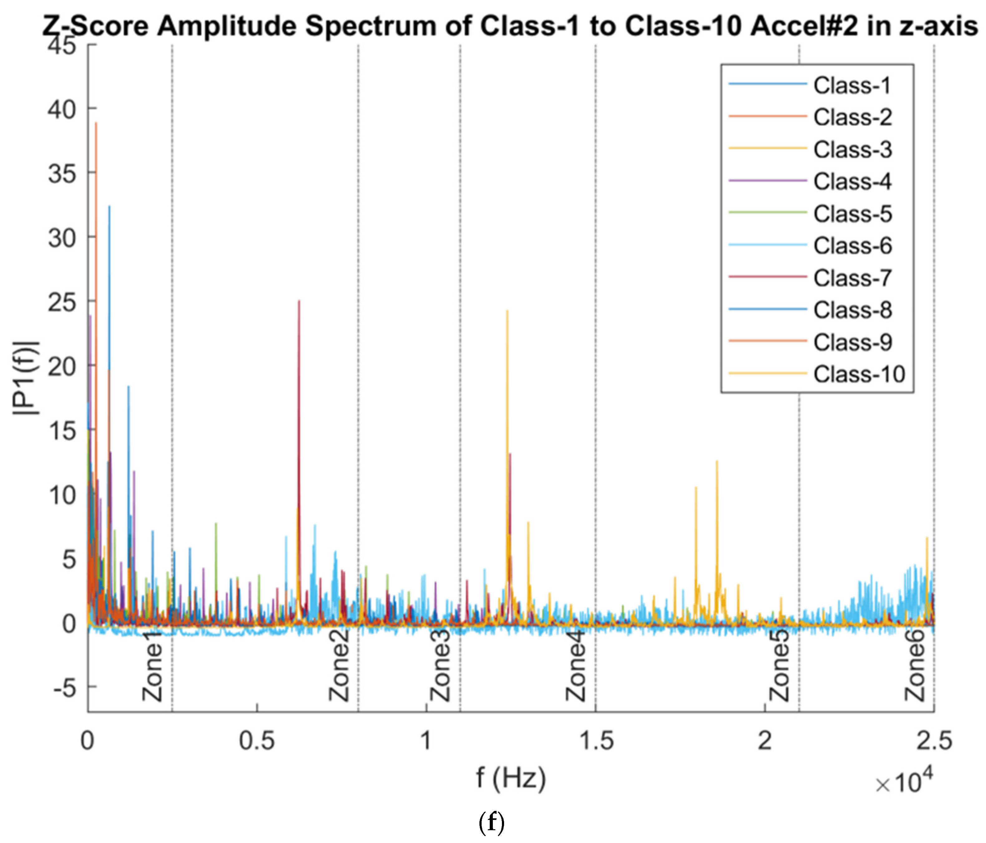
3.4.2. Frequency Domain Data

All accelerometer data was converted into the Frequency Domain using a Fast Fourier Transform. By learning the characteristics of these signals in the frequency domain, the optimal sample window and different power bands could be determined. To evaluate data effectively, all the data needs to remove offset or DC components before converting data into a frequency domain. A high-pass Filter was applied to all accelerometer data before converting it into the Frequency Domain.

Figure 6 presents six distinct frequency zones, labeled Zone 1 to Zone 6, each representing a group with similar frequency characteristics when comparing the frequency behavior across each axis of the accelerometers. These zones effectively capture different frequency patterns and can be used as distinct power bands for further analysis.

3.4.3. Sample Window

Using a too large sample window would cause the system to miss certain frequency behaviors, while using a too small sample window would cost additional computational power. From the Frequency Domain analysis, each frequency characteristic is around 1 kHz or 1000 samples or a frame of 0.02 s. Hence, the selected sample window is 1000 samples with a standard overlap of 50%.

3.4.4. Power Band

From the Frequency Domain analysis, six different frequency zones capture different frequency characteristics; hence, these frequency zones were selected as six different power bands. Band 1 is from 0 to 2.5 kHz, band 2 is from 2.5 kHz to 8 kHz, band 3 is from 8 kHz to 11 kHz, band 4 is from 11 kHz to 15 kHz, band 5 is from 15 kHz to 21 kHz, and band 6 is from 21 kHz to 25 kHz. These bands are labeled in 6 different zones in Figure 6 above.

3.4.5. 58 Predictors

From eight available time-domain data, 58 predictors were created with average and variance using the tachometer, microphone, and all accelerometer data in the three axes, the number of zero-crossing and six different power bands from the accelerometer data. Average and variance information from tachometer data should not be needed for machine learning because the rotating frequency from the tachometer should be similar or the same. However, these two predictors were not removed so we could confirm their importance when finding the most important predictors for the study.

4. Decision Tree and Important Predictors

4.1. Initial Decision Tree and 11 Important Predictors

The Decision Tree machine-learning model was evaluated to confirm the prediction quality and list important predictors before exploring other models later using MATLAB 2022b Classification Learner. This method was chosen because it is easy to create by programming via MATLAB and easy to understand. It also does not require standardizing or Z-score all predictors before training the model; hence, there is no need to worry about whether data is categorical or number. It also has a flexible boundary with good prediction quality.

For this model, all 59 predictors were studied. The Entropy method was used to determine the most informative information, and the binary split method was used to improve the prediction quality. To find the best Number of Splits for the Decision Tree model, 1000 different Decision Tree models with the Number of Splits ranging from 9 to 1000 were created. The minimum Number of Splits must be the total number of classes subtracted by 1. A higher maximum Number of Splits could be explored. However, 1000 is good enough for this study. Then, the average F-score of all ten classes for each model was compared, and the best Number of Splits was chosen.

The best average F-score is 99.8% at the Number of Splits of 30. From Figure 7, as the Number of Splits increases, the average F-score increases but flat out at the Number of Splits of 30. The prediction quality of the Decision Tree with the Number of Split at 30 is very good, with all the outcomes staying close to 99% or 100% as shown in

Table 4. Prediction Quality of Decision Tree Model.

Class	Accuracy	Precision	Recall	F-Score
1	99.96%	99.8%	99.8%	99.8%
2	99.92%	99.402%	99.8%	99.601%
3	99.88%	99.4%	99.4%	99.4%
4	99.98%	100%	99.8%	99.9%
5	99.96%	99.8%	99.8%	99.8%
6	100%	100%	100%	100%
7	100%	100%	100%	100%
8	99.98%	100%	99.8%	99.9%
9	99.92%	99.6%	99.6%	99.6%
10	100%	100%	100%	100%

. Both the Confusion Matrix and ROC curves also show excellent performance as it can be seen in Table 4 and Figure 8 and Figure 9.

Using the Decision Tree Important Predictors, there are 11 most significant predictors in this study, whose estimates are much higher than the rest of the predictors. The next lower predictor has an estimate that is 63% lower than the 11th most significant predictor seen in Figure 10. Hence, the top 11 predictors are labeled as the most important for this study. Those 11 predictors are: predictor 22nd as the Number of Zero Cross in the overhang accelerometer in the z-axis, predictor 31st as Power Band two in underhang accelerometer in the z-axis, predictor 12th as the variance of underhang accelerometer in the y-axis, predictor 15th as the variance of overhang accelerometer in the y-axis, predictor 38th as power band three in overhang accelerometer in the x-axis, predictor 57th as power band 6 in overhang accelerometer in the y-axis, predictor 11th as the variance of underhang accelerometer in the x-axis, predictor 25th as power band 1 of underhang accelerometer n z-axis, predictor 16th as the variance of overhang accelerometer in the z-axis, predictor 37th as power band 3 in underhang accelerometer in the z-axis, and predictor 13th as variance in underhang accelerometer in the z-axis.

All 11 predictors are not involved with tachometer data as expected because they only provide the same rotating frequency. This indicates that microphone data is not necessary.

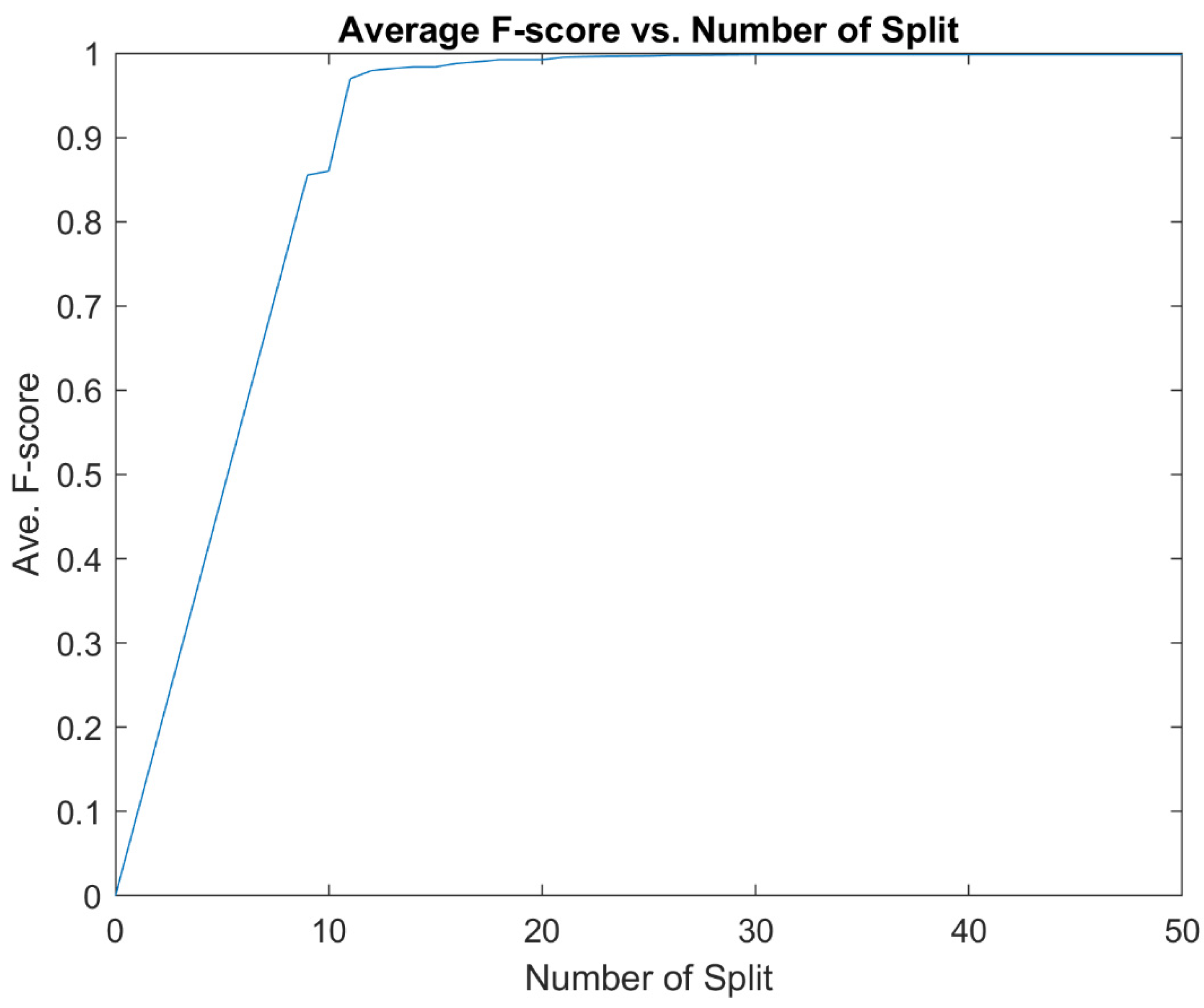
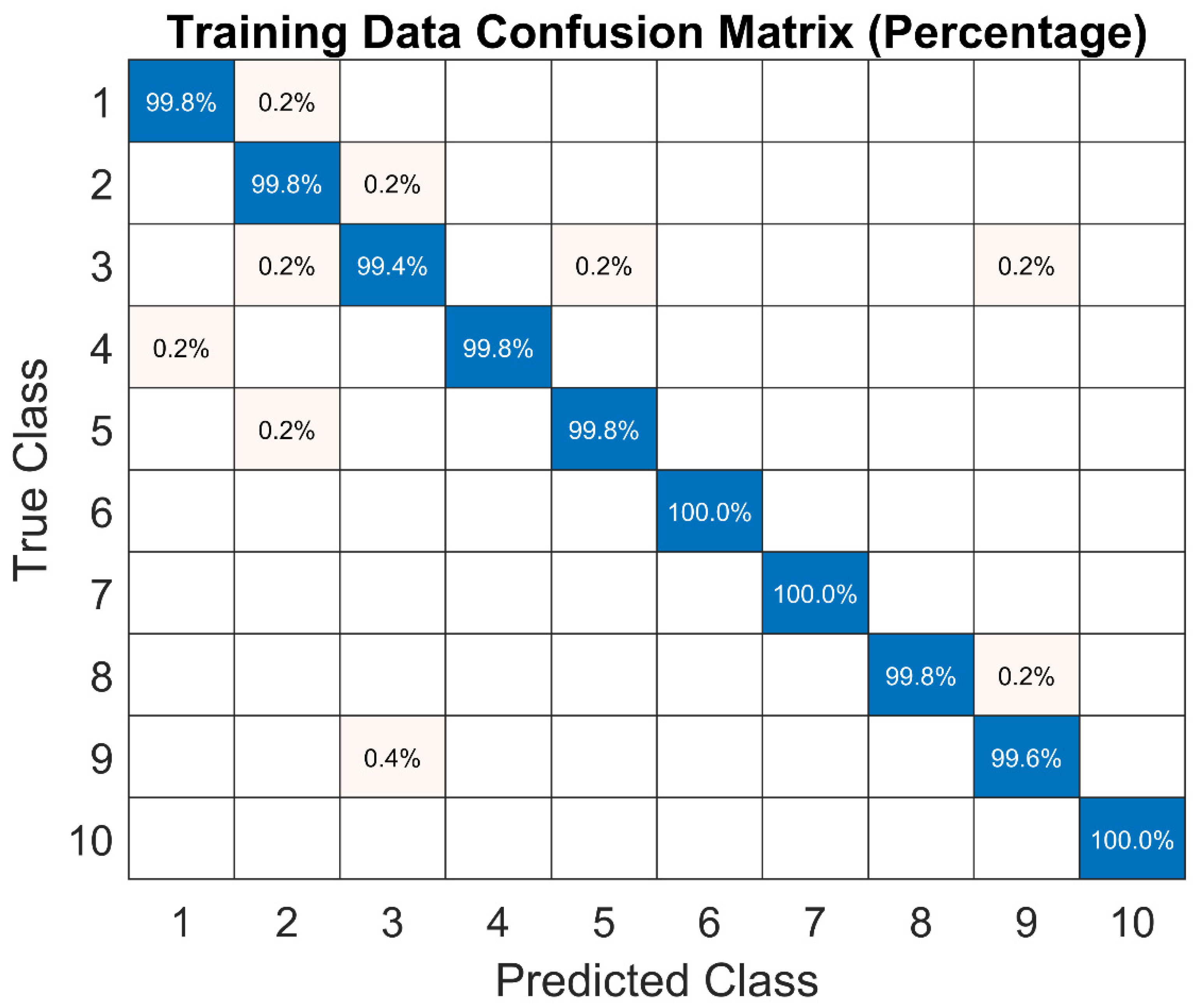
4.2. Improved Decision Tree Model with 11 Predictors

An improved Decision Tree model was created using 11 predictors instead of all 58 predictors. As they can be seen in

Table 5. Prediction Quality of IMPROVED Decision Tree Model.

Class	Accuracy	Precision	Recall	F-score
1	99.96%	100%	99.8%%	99.6%
2	99.92%	99.206%	99.602%	100%
3	99.82%	98.614%	99.104%	99.6%
4	99.96%	99.8%	99.8%	99.8%
5	99.92%	100%	99.598%	99.2%
6	100%	100%	100%	100%
7	99.99%	99.599%	99.499%	99.4%
8	99.94%	99.8%	99.7%	99.6%
9	99.98%	100%	99.9%	99.8%
10	100%	100%	100%	100%

and through Figure 11 and Figure 12, the prediction quality, confusion Matrix, and ROC curves showed compatible results.

5. Explore Different Machine Learning Models with ClassificationLearner

This section discusses the results of the analysis obtained using the MATLAB ClassificationLearner. The Cross-Validation is chosen 10-fold. 20% of data is set aside as Test Data.

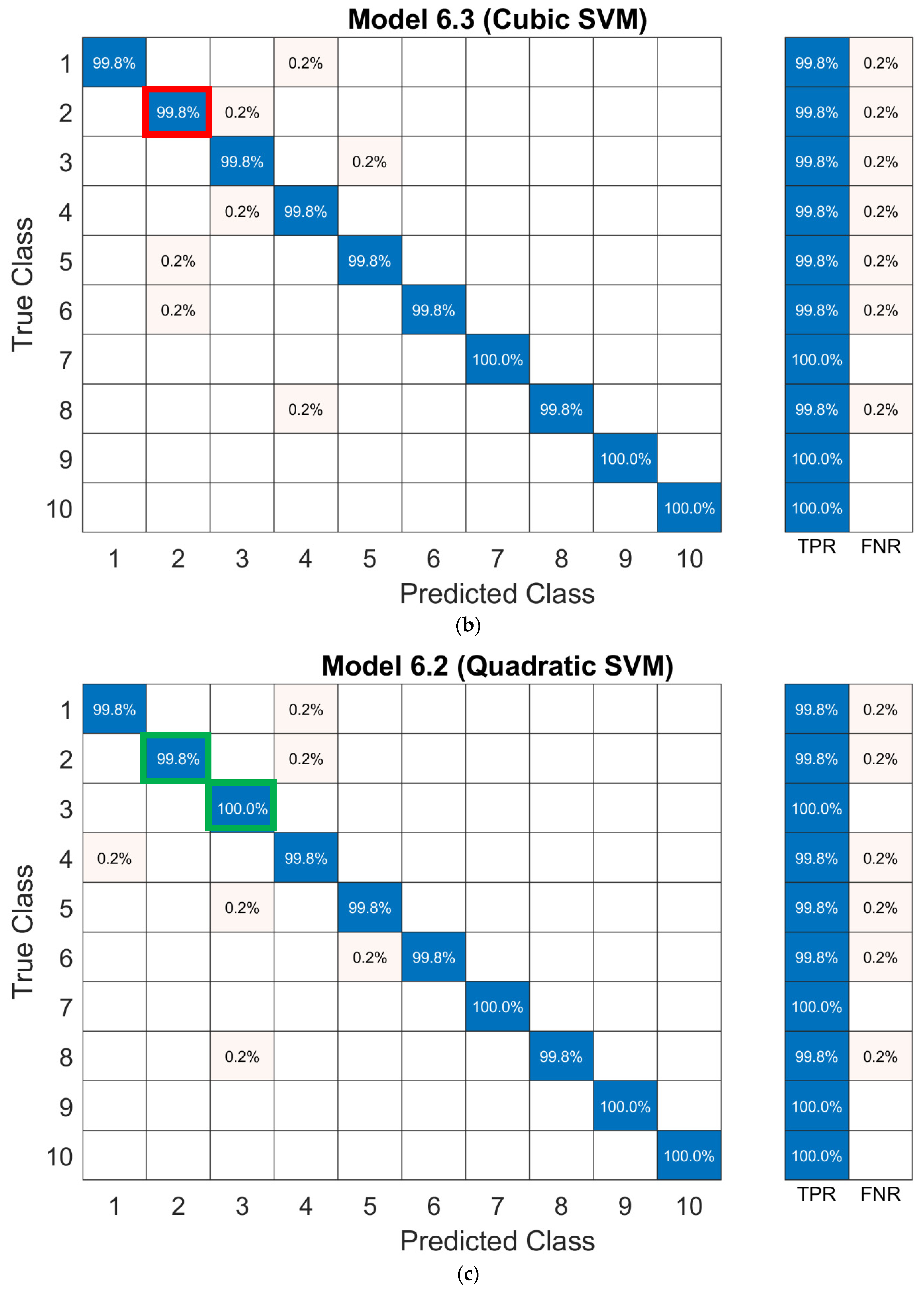
5.1. Classification Learner with All 58 Predictors

All 58 predictors were tested with all available machine-learning models in MATLAB ClassificationLearner. As displayed in

Table 6. Summary of Accuracy for the Trained Model Using All Predictors in MATLAB Classification Learner.

Model Number	Model Type	Neural Network	Predictors	Accuracy (Validation)
3.1	Decision Tree	Fine Tree	All	99.1%
3.2	Decision Tree	Medium	All	98.9%
3.3	Decision Tree	Coarse Tree	All	50.0%
4.1	Linear Discriminant	Linear Discriminant	All	99.1%
5.2	Naïve Bayes	Kernel Naïve Bayes	All	87.7%
6.1	SVM	Linear SVM	All	99.8%
6.2	SVM	Quadratic SVM	All	99.8%
6.3	SVM	Cubic SVM	All	99.8%
6.4	SVM	Fine Gaussian SVM	All	41.0%
6.5	SVM	Medium Gaussian SVM	All	99.3%
6.6	SVM	Coarse Gaussian SVM	All	99.6%
7.1	KNN	Fine KNN	All	99.0%
7.2	KNN	Medium KNN	All	97.9%
7.3	KNN	Coarse KNN	All	91.0%
7.4	KNN	Cosine KNN	All	98.6%
7.5	KNN	Cubic KNN	All	97.4%
7.6	KNN	Weighted KNN	All	98.4%
8.1	Kernel	SVM Kernel	All	92.4%
8.2	Kernel	Logistic Regression Kernel	All	91.5%
9.1	Ensemble	Boosted Trees	All	99.4%
9.2	Ensemble	Bagged Trees	All	99.4%
9.3	Ensemble	Subspace Discriminant	All	98.1%
9.4	Ensemble	Subspace KNN	All	91.4%
9.5	Ensemble	RUS Boosted Trees	All	98.9%
10.1	Neural Network	Narrow Neural Network	All	99.3%
10.2	Neural Network	Medium Neural Network	All	99.4%
10.3	Neural Network	Wide Neural Network	All	99.5%
10.4	Neural Network	Bilayer Neural Network	All	99.3%
10.5	Neural Network	Trilayered Neural Network	All	99.4%

, the three best models are from Support Vector Machine (SVM): Linear, Quadratic, and Cubic, with an accuracy of 99.8%.

To choose the best possible model from the Linear, Quadratic, and Cubic SVM, a closer observation of their Confusion Matrix was needed. Model 6.2 of the Quadratic SVM has a slightly better performance with Class 2 and Class 3 than the Linear and Cubic SVM. For the Quadratic SVM, these two classes have 99.8% and 100% accuracy, which are higher than the other two models at 99.5% and 99.8% respectively. The differences are highlighted in the Figure 13 below, with red boxes indicating lower accuracy and green boxes indicating higher accuracy.

5.2. Improved Quadratic SVM Model with 58 Predictors

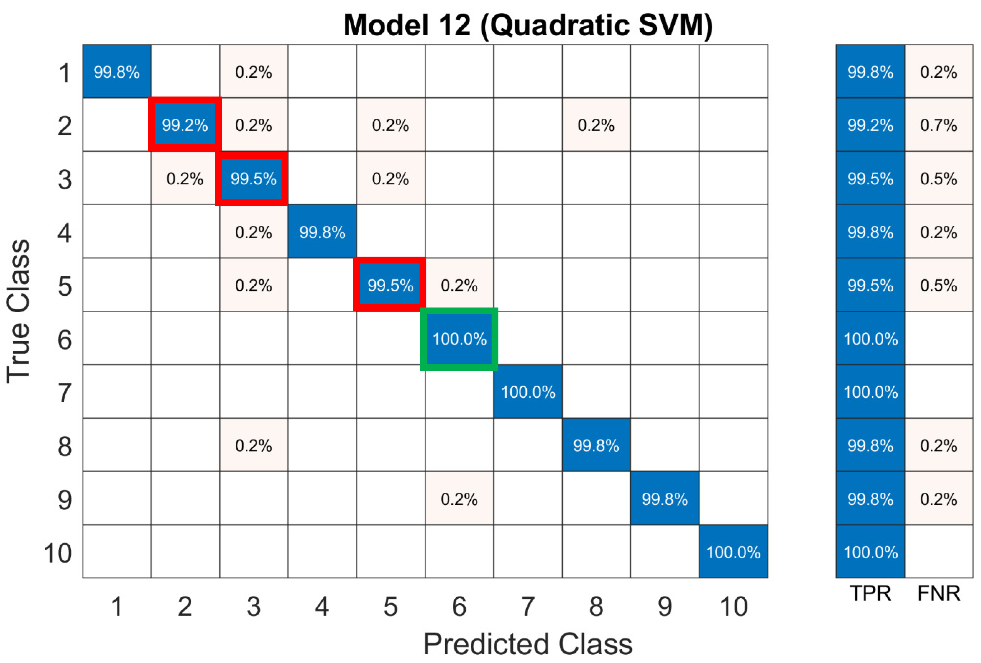
To improve the existing Quadratic SVM Model with all 58 predictors, a new Quadratic SVM Model was created but using only 11 important predictors found during the Decision Tree Study.

Table 7. Quadratic SVM Models using All Predictors vs. 11 Predictors.

Model Number	Model Type	Neural Network	Predictors	Accuracy (Validation)	Training Time
6.2	SVM	Quadratic SVM	All	99.8%	16.3 s
12	SVM	Quadratic SVM	Only 11 Predictors	99.7%	6.9 s

shows the model performance in terms of accuracy and training time.

The overall accuracy of the improved Quadratic SVM decreases slightly by 0.1%, from 99.8% to 99.7%, with accuracy differences highlighted in the confusion matrix of Figure 14 which uses green boxes for higher accuracy and red boxes for lower accuracy. Despite the minor decrease in prediction quality, the training time for the SVM model with 11 predictors is 57% shorter compared to the model with all 58 predictors.

6. Model Evaluation

The final best model for this study is Quadratic SVM, using the 11 most important predictors with an overall accuracy of 99.7% and a total training time of 6.9 s. Even though the accuracy decreases by 0.1% from the Quadratic SVM using all 58 predictors, the amount of training time it saves is significant. One of the earlier obstacles during this study is computational power. With fewer predictors, a more extensive data set could be used to generalize the proposed system.

To assess the performance of the Quadratic SVM model on unseen data, a random subset from the original dataset was extracted and used as a new test set. The accuracy dropped significantly when evaluated on this new data, suggesting that the initial training dataset was insufficient or not diverse enough to capture the full range of features required for the model to generalize well. Thus, this result may seem to be due to a potential issue with overfitting, where the model may have learned to perform exceptionally well on the training data but struggles to generalize to new, unseen data. But, we believe that the drop in performance may be due to the varying frequency of the motors. This is why, in our initial dataset selection, the key parameter for selection was the rotational frequency. If the rotational frequency changes, this causes tremendous variation. In our experiment, we were able to verify when the frequency was similar in another dataset; although the model and predictors may be different, the performance was comparable to the initial results, which shows that when the frequencies are similar, high classification accuracy could be obtained. Therefore, if a form of time-domain signal warping could be applied to absorb the variation caused by the change in frequency, the algorithm could produce higher accuracy.

For verification, a few additional Quadratic SVM models using two different datasets (data sets #2 and #3) of equal size and modified predictors were trained. Similar to Cross-Validation in the initial training, 20% of each new data set is set aside for testing. And again, both models showed a significant drop in test accuracy shown in

Table 8. Summary of Quadratic SVM Models Using All Predictors vs. 11 Predictors Across Three Different Datasets.

Model#	Trained Data Set	Classifier	Classifier Type	Predictors	Training Accuracy (Validation)	Test with Data Set#1	Test with Data Set#2	Test with Data Set#3
Version#1-6.2	Data Set#1(1)	SVM	Quadratic SVM	All	99.80%	100.00%	15.10%	19.50%
Version#1-12	Data Set#1	SVM	Quadratic SVM	Predictor set#1(4)	99.70%	99.90%	18.50%	21.40%
Version#2-#1	Data Set #2 (2)	SVM	Quadratic SVM	All	99.80%	25.90%	99.80%	44.60%
Version#2-#3	Data Set #2	SVM	Quadratic SVM	Predictor set#2(5)	99.80%	20.00%	100.00%	47.60%
Version#3-#3	Data Set #3(3)	SVM	Quadratic SVM	All	99.80%	23.50%	46.70%	99.90%
Version#3-#4	Data Set #3	SVM	Quadratic SVM	Predictor set#3(6)	99.80%	30.30%	56%	99.90%

. This further reinforces the hypothesis that the datasets currently in use may be too small or not representative enough of the underlying patterns in the data. The main reason for the poor model performance may have been due to the limited size of the training data, which in turn was constrained by the similarity in frequency of the data and available computational power. The lack of sufficient processing capability made training and testing the model on larger, more comprehensive datasets impossible. Since the computer used for this task lacked the necessary computing and memory resources to handle large-scale data processing, this became a significant bottleneck, limiting both the quantity and quality of data that could be fed into the model. With smaller datasets, the model may not encounter enough feature variation, reducing its ability to learn effectively and to generalize to unseen data. This lack of diversity in the training data can lead to overfitting, where the model performs exceptionally well on the training set but struggles to adapt to new patterns when tested on different data.

(1)

Data Set#1: first 2,500,000 records

(2)

Data Set#2: random 2,500,000 records with random record indexes: 40, 45, 7, 45, 31, 5, 14, 27, 47, 42

(3)

Data Set#3: random 2,500,000 records with random record indexes: 33, 2, 44, 46, 33, 38, 37, 20, 33, 8

(4)

Predictor Set#1:

#22. numZeroCross_2z, #31. BandPower2_1z, #12. Var_1y, #15. Ver_2y, #38. BandPower3_3x, #57. BandPower6_2y, #11. Var_1x, #25. BandPower1_1z, #16. Var_2z, #37. BandPower3_1z, #13. Var_1z

(5)

Predictor Set#2:

#53. BandPower6_1x, #11. Var_1x, #15. Var_2y, #56. BandPower6_2x, #32. BandPower2_2x, #12. Var_1y, #13. Var_1z, #54. BandPower6_1y, #6. Avg_1y, #1. Avg_tach, #2. Avg_mic

(6)

Predictor Set#3:

#53. BandPower6_1x, #16. Var_2z, #15. Var_2y, #54. BandPower6_1y, #14. Var_2x, #12. Var_1y, #13. Var_1z, #11. Var_1x, #9. Avg_2y, #1. Avg_tach, #2. Avg_mic

To improve model performance, the first priority is to increase the size and diversity of the training data, allowing the model to capture more complex patterns and reduce overfitting. Additionally, refining feature sets through careful feature engineering can enhance the model’s generalization ability. Cross-validation should be implemented to ensure more reliable model evaluation and regularization techniques can be applied to mitigate overfitting by penalizing overly complex models. If these steps do not yield sufficient improvements, exploring alternative machine learning algorithms, such as Random Forests or Neural Networks, may better handle the data’s non-linear patterns.

7. Conclusions

This paper presents case study results where a machine learning model was developed to detect ten different conditions of a rotating machine using only acceleration data with the MATLAB Classification Learner Application. In this study, two approaches were explored: (1) programming a Decision Tree model in MATLAB and (2) using MATLAB Classification Learner to identify the best-performing model. The results showed that acceleration data alone is sufficient for detecting machine conditions without the need for additional sensors like tachometers or microphones. The Quadratic Support Vector Machine (SVM) was the top model, achieving over 99.7% accuracy using just 11 key predictors while reducing training time by over 60% compared to models using all 58 predictors.

However, when evaluating the model on new datasets, a significant drop in test accuracy was observed, indicating several reasons for the drop. Often, this is because the original training data may not have been diverse enough to generalize well to unseen data. Additional models trained on different datasets faced similar declines, highlighting a potential need for a larger and more representative dataset for generalization. But, again, this may be due to the difference in the data frequency as the dataset with similar frequency was initially chosen for training, verification and testing. The following steps will focus on expanding the training dataset to include more diverse records and improving feature selection to better capture the important patterns. But again, it is important to note that one of the key parameters for selection was the rotational frequency. If the rotational frequency changes, this can create tremendous variation in predictor characterization. Therefore, dynamic time warping could be applied to absorb the variation caused by the change in frequency and other regularization techniques to address the potential overfitting.

References

1. Riberiro, F.; Marins, M.; Sergio, N.; Eduardo, S. Rotating Machinery Fault Diagnosis using Similarity-based Model. Simp. Bras. Telecomunicac Oese Process. Sinais 2017, 35, 277–281. [Google Scholar] [CrossRef]
2. Liu, J.; Wang, W.; Golnaraghi, F. An Enhanced Diagnostic Scheme for Bearing Condition Monitoring. IEEE Trans. Instrum. Meas. 2010, 59, 309–321. [Google Scholar] [CrossRef]
3. Li, P.; Kong, F.; He, Q.; Liu, Y. Multiscale Slope Feature Extraction for Rotating Machinery Fault Diagnosis using Wavelet Analysis. Measurement 2013, 46, 497–505. [Google Scholar] [CrossRef]
4. Li, B.; Zhang, P.; Liu, D.; Mi, S.; Ren, G.; Tian, H. Feature Extraction for Rolling Element Bearing Fault Diagnosis Utilizing Generalized S Transform and Two-Dimensional Non-Negative Matrix Factorization. J. Sound Vib. 2010, 330, 2388–2399. [Google Scholar] [CrossRef]
5. Rauber, T.W.; de Assis Boldt, F.; Varejao, F.M. Heterogeneous Feature Models and Feature Selection Applied to Bearing Fault Diagnosis. IEEE Trans. Ind. Electron. 2015, 62, 637–646. [Google Scholar] [CrossRef]
6. Wu, S.-D.; Wu, P.-H.; Wu, C.-W.; Ding, J.-J.; Wang, C.-C. Bearing Fault Diagnosis Based on Multiscale Permutation Entropy and Support Vector Machine. Entropy 2012, 14, 1343–1356. [Google Scholar] [CrossRef]
7. Tong, Z.; Wei, L.; Zhang, B.; Gao, H.; Zhu, X.; Zio, E. Bearing Fault Diagnosis Based on Discriminant Analysis Using Multi-View Learning. Mathematics 2022, 10, 3889. [Google Scholar] [CrossRef]
8. Alexakos CKarnavas, Y.; Drakaki, M.; Tziafettas, I. A Combined Short Time Fourier Transform and Image Classification Transformer Model for Rolling Element Bearings Fault Diagnosis in Electric Motors. Mach. Learn. Knowl. Extr. 2021, 3, 228–242. [Google Scholar] [CrossRef]
9. Tran, T.; Lundgren, J. Drill Fault Diagnosis Based on The Scalogram and MEL Spectrogram of Sound Signals using Artificial Intelligence. IEEE Access 2020, 8, 203655–203666. [Google Scholar] [CrossRef]
10. Li, C.; Sánchez, R.-V.; Zurita, G.; Cerrada, M.; Cabrera, D. Fault Diagnosis for Rotating Machinery Using Vibration Measurement Deep Statistical Feature Learning. Sensors 2016, 16, 895. [Google Scholar] [CrossRef] [PubMed]
11. Zhen, J. Rotating Machinery Fault Diagnosis Based on Adaptive Vibration Signal Processing under Safety Environment Conditions. Math. Probl. Eng. 2022, 2022, 1543625. [Google Scholar] [CrossRef]
12. Rajabi, S.; Azari, M.S.; Santini, S.; Flammini, F. Fault Diagnosis in Industrial Rotating Equipment Based on Permutation Entropy, Signal Processing and Multi-Output Neuro-Fuzzy Classifier. Expert Syst. Appl. 2022, 206, 117754. [Google Scholar] [CrossRef]
13. Mba, D.; Cooke, A.; Roby, D.; Hewitt, G. Opportunities Offered by Acoustic Emission for Shaft-Steal Rubbing in Power Generation Turbines: A Case Study. In Proceedings of the International Conference on Condition Monitoring, Oxford, UK, 2–4 July 2003; pp. 2–4. [Google Scholar]
14. Kim, Y.; Tan, A.; Mathew, J.; Yang, B. Experimental Study on Incipient Fault Detection of Low-Speed Rolling Element Bearings: Time Domain Statistical Parameters. In Proceedings of the 12th Asia-Pacific Vibration Conference, Sapporo, Japan, 6–9 August 2007; pp. 6–9. [Google Scholar]
15. Kim, E.; Tan, C.A.; Mathew, J.; Kosse, V.; Yang, B.-S. A Comparative Study on The Application of Acoustic Emission Technique and Acceleration Measurements for Low-Speed Condition Monitoring. In Proceedings of the 12th Asia-Pacific Vibration Conference, Sapporo, Japan, 6–9 August 2007; pp. 1–11. [Google Scholar]
16. Mba, D. The Detection of Shaft-Seal Rubbing in Large-Scale Turbines using Acoustic Emission. In Proceedings of the 14th International Congress on Condition Monitoring and Diagnostic Engineering Management (COMADEM’2001), Manchester, UK, 4–6 September 2001; pp. 21–28. [Google Scholar]
17. Tan, C.K.; Mba, D. Limitation of Acoustic Emission for Identifying Seeded Defects in Gearboxes. J. Nondestruct. Eval. 2005, 24, 11–28. [Google Scholar] [CrossRef]
18. Altaf, M.; Uzair, M.; Naeem, M.; Ahmad, A.; Badshah, S.; Shah, J.A.; Anjum, A. Automatic and Efficient Fault Detection in Rotating Machinery using Sound Signals. Acoust. Aust. 2019, 47, 125–139. [Google Scholar] [CrossRef]
19. Hong, G.; Suh, D. Mel Spectrogram-Based Advanced Deep Temporal Clustering Model with Unsupervised Data for Fault Diagnosis. Expert Syst. Appl. 2023, 217, 119551. [Google Scholar] [CrossRef]
20. Gundewar, S.K.; Kane, P.V. Rolling Element Bearing Fault Diagnosis using Supervised Learning Methods—Artificial Neural Network and Discriminant Classifier. Int. J. Syst. Assur. Eng. Manag. 2022, 13, 2876–2894. [Google Scholar] [CrossRef]
21. Shubita, R.R.; Alsadeh, A.S.; Khater, I.M. Fault Detection in Rotating Machinery Based on Sound Signal Using Edge Machine Learning. IEEE Access 2023, 11, 6665–6672. [Google Scholar] [CrossRef]
22. Jalayer, M.; Orsenigo, C.; Vercellis, C. Fault Detection and Diagnosis for Rotating Machinery: A Model Based on Convolutional LSTM, Fast Fourier and Continuous Wavelet Transforms. Comput. Ind. 2021, 125, 103378. [Google Scholar] [CrossRef]
23. Inyang, U.I.; Petrunin, I.; Jennions, I. Diagnosis of Multiple Faults in Rotating Machinery Using Ensemble Learning. Sensors 2023, 23, 1005. [Google Scholar] [CrossRef] [PubMed]
24. Das, O.; Bagci Das, D.; Birant, D. Machine Learning for Fault Analysis in Rotating Machinery: A Comprehensive Review. Heliyon 2023, 9, 6. [Google Scholar] [CrossRef] [PubMed]
25. NMB Technologies. What is a Ball Bearing? Available online: https://nmbtc.com/white-papers/what-is-a-ball-bearing/ (accessed on 1 November 2022).
26. Machinery Fault Dataset. Kaggle. Available online: https://www.kaggle.com/datasets/uysalserkan/fault-induction-motor-dataset/discussion/361583 (accessed on 1 November 2022).
Figure 1. Diagram displaying the workflow of the study.
Algorithms 17 00441 g001
Figure 2. Bearings and its parts: outer ring, cage, steel balls, and inner rings [25].
Algorithms 17 00441 g002
Figure 3. Bearing faults: inner race fault (left), outer race fault (center), and ball fault (right) [8].
Algorithms 17 00441 g003
Figure 4. Simulator setup to collect data in F. Ribeiro’s study [10].
Algorithms 17 00441 g004
Figure 5. Sensor data in Time Domain: (a) Tachometer data (b) Microphone data (c) Underhang Accelerometer Data in 3 axes, and (d) Overhang Accelerometer Data in 3 axes.
Algorithms 17 00441 g005aAlgorithms 17 00441 g005b
Figure 6. Frequency Domain Data across all 10 classes (a) Underhang Accelerometer in the x-axis (b) Underhang Accelerometer in the y-axis (c) Underhang Accelerometer in the z-axis (d) OVerhang Accelerometer in the x-axis (e) Overhang Accelerometer in the y-axis (f) Overhang Accelerometer in the z-axis.
Algorithms 17 00441 g006aAlgorithms 17 00441 g006bAlgorithms 17 00441 g006cAlgorithms 17 00441 g006d
Figure 7. Average F-score vs. Number of Splits in 1000 Decision Tree with a Number of Split from 0–50.
Algorithms 17 00441 g007
Figure 8. Confusion Matrix of Decision Tree Model.
Algorithms 17 00441 g008
Figure 9. Receiver Operating Characteristic curve of the Decision Tree model.
Algorithms 17 00441 g009
Figure 10. Top 11 predictors with the highest significance estimates using the Decision Tree method.
Algorithms 17 00441 g010
Figure 11. Confusion Matrix of Improved Decision Tree Model.
Algorithms 17 00441 g011
Figure 12. Receiver Operating Characteristic curve of Improved Decision Tree model.
Algorithms 17 00441 g012
Figure 13. Comparison of Linear, Cubic, and Quadratic SVMs, highlighting the slight accuracy advantage of the Quadratic SVM. (a) Linear SVM, (b) Cubic SVM, with red boxes indicating lower accuracy, and (c) Quadratic SVM, with green boxes indicating higher accuracy.
Algorithms 17 00441 g013aAlgorithms 17 00441 g013b
Figure 14. Improved Quadratic SVM model using 11 predictors, with green boxes indicating accuracy improvement and red boxes for lower accuracy compared to the Quadratic SVM using all predictors.
Algorithms 17 00441 g014