Performance Analysis and Parallel Scalability of Numerical Methods for Fractional-in-Space Diffusion Problems with Adaptive Time Stepping

Abstract

We study numerical methods and algorithms for time-dependent fractional-in-space diffusion problems. The considered anomalous diffusion is modelled by the fractional Laplacian ${(-\Delta )}^{\alpha }$, $0<\alpha <1$, following the integral definition. Fractional diffusion is non-local, and the finite element method (FEM) discretization in space leads to a dense stiffness matrix. It is well known that numerically solving such non-local boundary value problems is expensive. Difficulties increase significantly when the problem is time-dependent. The aim of the article is to develop computationally efficient methods and algorithms. There are two main features of our approach. Hierarchical semi-separable (HSS) compression is applied for an approximate solution of the arising linear systems. For time discretization, we use an adaptive forward–backward Euler scheme. The properties of the composite algorithm thus obtained are investigated. In particular, the block representation of HSS compression allowed us to upgrade the HSS solver to efficiently handle varying diagonally perturbed transition matrices corresponding to changing time steps. The contribution of the paper is threefold. The methods are completely constructive, which allows for a clearly structured description of the algorithms. A theoretical estimate of the computational complexity is presented. It shows the advantages of the adaptive time stepping in combination with the HSS solver. Theoretical results are supported by representative numerical experiments. Both sequential and parallel scalability and efficiency are analyzed. The presented results provide convincing proof of the concept of the proposed methods and algorithms.

1. Introduction

Anomalous diffusion has many applications in science and engineering. It is observed in flows in strongly heterogeneous porous media, superconductivity, diffusion of polymers in supercold media [1]; the electrodiffusion of ions into nerve cells [2] and photon diffusion diagnostics [3]; image processing and machine learning [4]; and the spread of viral diseases, computer viruses, and crime [5], to name a few. A more exhaustive review of its applications can be found in [6]. Anomalous diffusion is mathematically modelled with the fractional Laplace operator ${(-\mathsf{\Delta })}^{\alpha }$, where $\alpha$ is the fractional power. There are different approaches regarding the definition of fractional Laplacian. For example, the Balakrishnan formula, a formula involving semi-group, and the Dynkins definition based on probabilistic considerations are discussed in [7,8]. It is shown that they are all equivalent in the whole space ${\mathbb{R}}^d$ but differ significantly when homogeneous Dirichlet boundary conditions in a bounded domain are enforced. The work of comparing the properties of relevant models is an ongoing process in which various aspects of nonlocal phenomena are analyzed as well as how they describe the available experimental data. In recent years, mathematicians have been particularly active in developing numerical methods for multidimensional boundary value problems in computational domains of general geometry, applying and comparing results for different definitions of fractional Laplacian. In [9], a comparison between the spectral and integral definitions can be found. In this work, we will concentrate on the following integral definition of ${(-\mathsf{\Delta })}^{\alpha }$:

$${\left(-\mathsf{\Delta }\right)}^{\alpha }u\left(x\right)=C\left(d,\alpha \right)\mathrm{P}.\mathrm{V}.{\int }_{{\mathbb{R}}^d}{\displaystyle \frac{u\left(x\right)-u\left(y\right)}{{|x-y|}^{d+2\alpha }}}dy,\alpha \in (0,1).$$

Here P.V. stands for principal value, d is the number of spatial dimensions, $\alpha$ is the fractional power, and $C(d,\alpha )$ is the following constant

$$C(d,\alpha )={\displaystyle \frac{2^{2\alpha }\alpha \Gamma \left(\alpha +\frac{d}{2}\right)}{{\pi }^{d/2}\Gamma (1-\alpha )}},$$

where $\Gamma$ is the gamma function. The fractional Laplacian is a non-local operator, and after applying a suitable discretization in space, the associated boundary value problems are reduced to solving systems of linear algebraic equations with dense matrices. For real-life problems, solving such systems can be computationally very expensive. If a standard LU or Cholesky decomposition is applied, the computational complexity to solve such a system is $O\left(N^3\right)$, where N is the number of degrees of freedom in space. For the considered parabolic problem, we need to solve a series of such linear systems, and the complexity becomes $O\left(m{N}^3\right)$, where m is the number of time steps. The aim of this research is to develop a more efficient numerical method with significantly less computational complexity.

In this work, we do not impose any special constraints on the geometry of the space computational domain $\Omega$. Also, in the finite element method (FEM) discretization, the mesh is unstructured by default. This formulation of the problem excludes the possibility of using more specialized linear algebra methods, which are based on a special structure of the stiffness matrix.

In computational mathematics, numerical methods for evolution problems are naturally based on the best available solvers for the corresponding elliptic boundary value problems. In the case of standard (local) diffusion, the stiffness matrix is sparse, and the developed near-optimal implicit methods for parabolic problems use fast preconditioned iterative solution methods (such as algebraic multigrid) for the emergent linear systems. The situation changes substantially when fractional diffusion is involved. The matrices are dense, and the concept of iterative solvers is not applicable in the general case. Furthermore, it turns out that there are specific difficulties depending on the definition of the fractional Laplacian used.

The history of the development of efficient (near-optimal) numerical methods for space-fractional diffusion problems in multidimensional domains of general geometry is less than ten years. And despite the considerable number of publications in this field, there are few results of this type for parabolic problems. Without pretending to be exhaustive, we will briefly touch on some of them. The case of spectral fractional diffusion is considered in [10,11,12,13,14]. The common feature of these results is that they can all be interpreted in terms of certain rational approximations. A further step in the development of this approach, significantly expanding the scope of the investigated problems, can be found in [15,16,17,18]. These works mainly focus on convergence analysis, with less discussion of algorithmic implementation and computational complexity. The same applies to [19], where finite element approximations for integral-fractional evolution problems are analysed. This paper is thematically closest to the parabolic equation we are considering.

Here, we use a rather different pure algebraic approach. Hierarchical semi-separable (HSS) compression is applied to approximately solve the arising linear systems. Earlier results based on HHS compression have been published in [20], where the case of a uniform time step is experimentally analysed.

In this paper, we implement an adaptive forward–backward Euler scheme for discretization in time. The aim is to automatically adapt the method to the evolution of the regularity of the solution. The obtained composite algorithm is analysed. The block representation of HSS compression is used to upgrade the HSS solver. This allows us to efficiently handle different diagonally perturbed transition matrices corresponding to changing time steps. The main contributions of the paper are as follows. The method is fully constructive, leading to a well-structured algorithmic implementation. The theoretical estimate of the computational complexity clearly shows the efficiency of the adaptive time stepping in combination with the HSS solver. The presented numerical experiments support the theoretical results. Both sequential and parallel scalability and efficiency are analyzed. The conclusion is that a convincing proof of concept of the proposed method and algorithm is presented.

In short, the fundamental novelties of the results that will be presented are the complex solutions obtained as a result of the developed composite algorithm. The time discretization is optimized, where the variable time step size adapts to the dynamics in the behavior of the solution. The hidden structure of the dense fractional diffusion stiffness matrix is shown to fit well with the stochastic HSS compression approach, thereby allowing attractive parallel scalability to be reached.

The rest of the paper is organized as follows. The fractional-in-space parabolic problem is presented in the next section, which concludes with the adaptive forward–backward Euler scheme for time discretization. Section 3 is devoted to hierarchical semi-separable compression. A key aspect here is the construction of a modified algorithm for diagonally perturbed matrices. The most important from a theoretical point of view is Section 4, where the computational complexity of the composite algorithm is analysed. The test problem for numerical experiments is then discussed in the next section. An analysis of the results of the conducted sequential and parallel numerical tests is presented in Section 6 and Section 7, respectively. In the next section, the relative error behaviour of the HSS solver is analyzed. The paper ends with a brief discussion of the results obtained.

2. Fractional-in-Space Parabolic Equation

2.1. Continuous Problem

The following parabolic problem with unknown function $u(x,t)$, $(x,t)\in \Omega \times [0,T]$ is considered

$$\left|\begin{array}{ccccc}\hfill {\displaystyle \frac{\partial u(x,t)}{\partial t}+{(-\Delta )}^{\alpha }u(x,t)}& =& f(x,t),\hfill & x\in \Omega ,\hfill & t\in (0,T)\hfill \\ \hfill u(x,t)& =& 0,\hfill & x\in {\Omega }^{\complement },\hfill & t\in (0,T)\hfill \\ \hfill u(x,0)& =& u^0\left(x\right),\hfill & x\in \Omega .\hfill \end{array}\right.$$

(1)

Here, $\Omega$ is the open space domain, ${\Omega }^{\complement }={\mathbb{R}}^d\setminus \Omega$ is the complement of $\Omega$, and the open time domain is denoted with $t\in (0,T)$.

2.2. Finite Element Approximation in Space

For the discretization in space of the ${(-\mathsf{\Delta })}^{\alpha }$ operator, we use a finite element scheme as outlined by Acosta in [21]. Let us consider an admissible triangulation on $\Omega$ with $N_{\mathcal{T}}$ as number of linear conforming elements. We will denote with $\{{\phi }_1,\dots ,{\phi }_N\}\subset {\mathbb{V}}_h$ the nodal basis corresponding to the internal nodes $\{x_1,\dots ,x_N\}$. The basis functions have the form ${\phi }_i\left(h_j\right)={\delta }_i^j,i,j\in [1,N]$, where $\delta$ is the Kronecker delta. Thus, the ${(-\mathsf{\Delta })}^{\alpha }$ operator (1) is approximated by the fractional stiffness matrix $K=\left(K_{ij}\right)\in {\mathbb{R}}^{N\times N}$ such that

$$K_{ij}={\displaystyle \frac{C(d,\alpha )}{2}}{\langle {\phi }_i,{\phi }_j\rangle }_{H^{\alpha }(\Omega )}.$$

where $H^{\alpha }(\Omega )$ is the following Sobolev space

$$H^{\alpha }(\Omega )=\{v\in L^2{(\Omega ):\left|v\right|}_{H^{\alpha }(\Omega )}<\infty \}.$$

It is defined with the Aronszajn–Slobodeckij seminorm

$${\left|v\right|}_{H^{\alpha }(\Omega )}={\left(\underset{\Omega \times \Omega }{\int \int }{\displaystyle \frac{{(v\left(x\right)-v\left(y\right))}^2}{{|x-y|}^{d+2\alpha }}}dxdy\right)}^{{\displaystyle \frac{1}{2}}}.$$

The integrals that must be calculated in order to compute $K_{ij}$ are carried out over the unbounded domain ${\mathbb{R}}^d$. A ball-shaped domain B is introduced around $\Omega$ to facilitate their calculations. The distance between the boundary $\partial \Omega$ and the compliment $B^{\complement }$ is discussed in [21]. An auxiliary admissible triangulation ${\mathcal{T}}_A$ is introduced on $B\setminus \Omega$ with $n_A$ elements. We will denote with $n_{\tilde{\mathcal{T}}}=n+n_A$ the number of elements on the combined triangulation $\tilde{\mathcal{T}}=\mathcal{T}\cup {\mathcal{T}}_A$. Thus, the coefficients of K can be written as

$$K_{ij}={\displaystyle \frac{C\left(d,\alpha \right)}{2}}\sum _{l=1}^{n_{\tilde{\mathcal{T}}}}\left(\sum _{k=1}^{n_{\tilde{\mathcal{T}}}}{I}_{l,k}^{i,j}+2J_l^{i,j}\right),l,k\in [1,n_{\tilde{\mathcal{T}}}].$$

The integrals I and J are

$$\begin{array}{cc}\hfill & I_{l,k}^{i,j}={\int }_{T_l}{\int }_{T_m}{\displaystyle \frac{\left({\phi }_i\left(x\right)-{\phi }_i\left(y\right)\right)\left({\phi }_j\left(x\right)-{\phi }_j\left(y\right)\right)}{{\left|x-y\right|}^{d+2\alpha }}}dxdy\hfill \\ \hfill & J_l^{i,j}={\int }_{T_l}{\int }_{B^{\complement }}{\displaystyle \frac{{\phi }_i\left(x\right){\phi }_j\left(x\right)}{{\left|x-y\right|}^{d+2\alpha }}}dydx.\hfill \end{array}$$

(2)

Computing $I_{l,k}^{i,j}$ and $J_k^{i,j}$ is a numerically complex task. For this purpose, specialized methods and algorithms are utilized. Specifically, singular integrands are involved in the computation of I, while J is calculated over an unbounded domain. The derivation of the I and J integrals as well as the theoretical analysis of the described finite element scheme is given in [21].

2.3. Backward Euler Discretization in Time

The unconditionally stable backward Euler scheme is implemented, in which the lumped mass matrix $M^L$ is used. $M^L$ is obtained by summing all off-diagonal elements of the mass matrix M into the diagonal. In this way,

$$M_{ii}^L=\sum _{j=0}^N{M}_{ij},i=1,\dots N,$$

and thus, the time-stepping method is written in the form

$$M^L{\displaystyle \frac{{\mathbf{u}}^{j+1}-{\mathbf{u}}^j}{{\tau }_j}}+K{\mathbf{u}}^{j+1}=M^L{\displaystyle \frac{{\mathbf{f}}^{j+1}+{\mathbf{f}}^j}{2}},j=0,\dots ,m-1.$$

(3)

Here, $\omega =\{t_0=0,t_1,\dots ,t_m=T\}$ is the finite difference mesh in the interval $[0,T]$, m is the number of time steps and ${\tau }_j$ the size of the jth step. The superscript j means that the value of the mesh function is taken at the node $t_j$. The implementation of the scheme (3) reduces to solving m systems of linear algebraic equations

$$\tilde{K}{u}^{j+1}={\tilde{b}}^{j+1},j=0,\dots m-1,$$

(4)

where

$${\tilde{K}}_j=K+{\displaystyle \frac{M^L}{{\tau }_j}},{\tilde{b}}^j=M^L\left({\displaystyle \frac{{\mathbf{f}}^{j+1}+{\mathbf{f}}^j}{2}}+{\displaystyle \frac{{\mathbf{u}}^j}{{\tau }_j}}\right).$$

Let us assume that the mesh of the time stepping scheme is uniform; that is, ${\tau }_j=\tau$. Then, the matrix ${\tilde{K}}_j=\tilde{K}$ does not depend on j, and if, for example, LU factorization is applied to solve the linear systems in (4), only one factorization of $\tilde{K}$ will be needed. The computational complexity of the factorization is $O\left(N^3\right)$ and the complexity of solving the system with the factorized matrix is $O\left(N^2\right)$. Thus, the computational complexity of the backward Euler scheme under consideration will be $O(N^3+m{N}^2)$. The parallel performance of LU- and HSS-based solvers for the case of a uniform time stepping is studied in [20].

The parameters ${\tau }_j$ control the time discretization error. When the regularity of the problem varies significantly with time, it may be advantageous to apply variable time steps, thus balancing the error. From a computational point of view, the motivation for using variable time steps is to significantly reduce their number compared to the uniform time step case while maintaining the required accuracy of the numerical solution. Such are, for example, the cases of an initial condition with jumps or jumps in time of the right-hand side. Let us assume that in a (by default) small number of subintervals of the time domain, we uniformly refine the step size. Then, the computational complexity of the LU-based solver method becomes $O(q{N}^3+m{N}^2)$, where q denotes the number of times to perform the LU factorization, which corresponds to the number of times, when ${\tau }_j\ne {\tau }_{j+1}$, including the first step ${\tau }_1$. The performance of this method for LU- and HSS-based solvers is examined in [22].

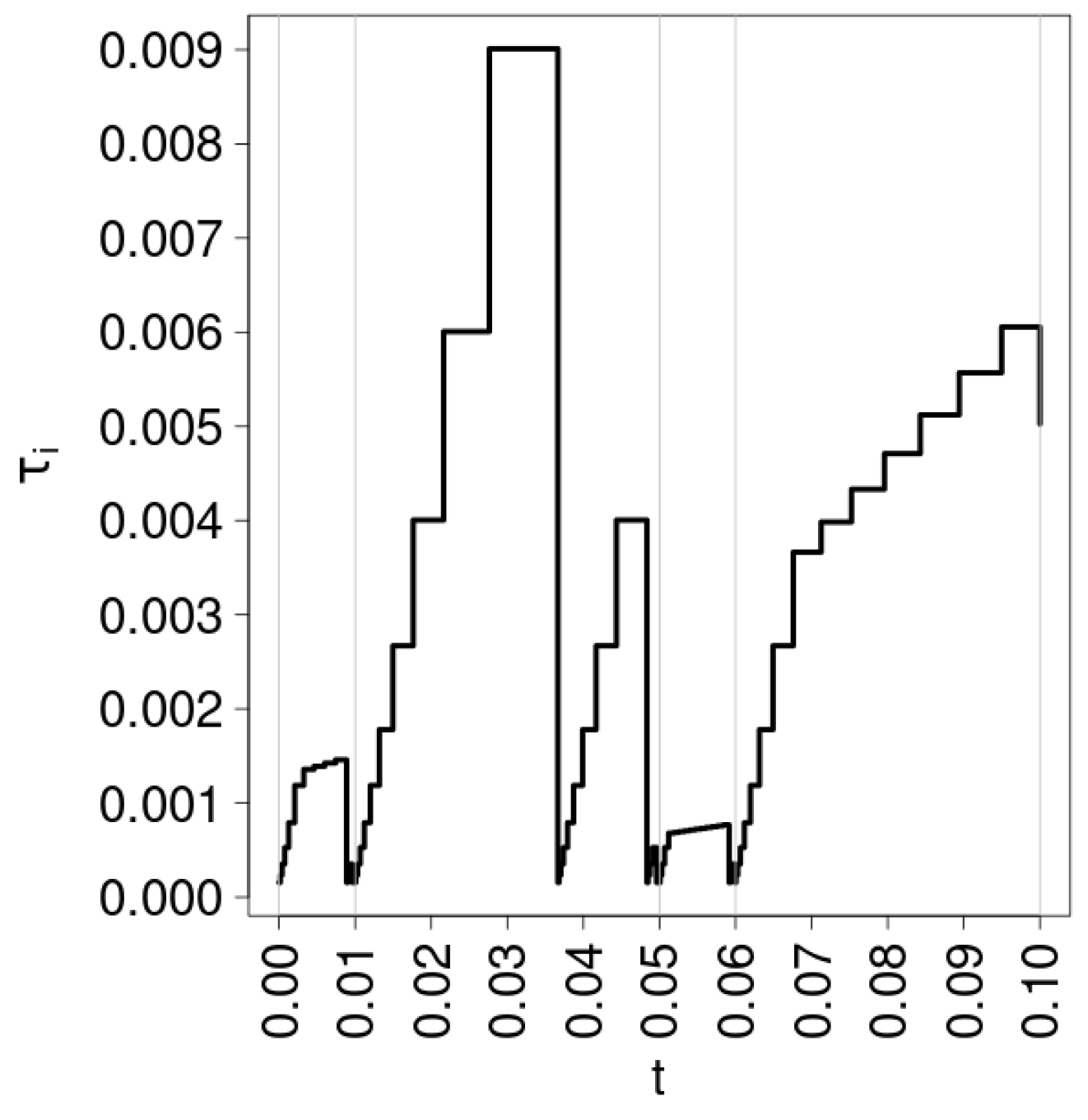
2.4. Adaptive Forward–Backward Euler Discretization in Time

The local refinement discussed above implies a more specific regularity of the solution in time that is a priori known. We do not need any such assumptions in this paper. The developed adaptive time stepping algorithm estimates the current error and automatically adjusts the next step size based on it. The procedure is as follows. The approximate solution is calculated using the stable backward Euler scheme (3), while a forward Euler scheme is used to estimate the size of the next time step. This type of methods are widely used in standard (local) diffusion problems. For example, adaptive time stepping for coupled multiscale problems is studied in [23,24], where the solution dynamics arise from nonlinear transitions of material properties. A parabolic equation with a jumping right-hand side is considered in [25], which is closest to the test problem we used in our numerical experiments. The time step adaptation algorithm explored in this paper is largely in the spirit of [25]. The great challenge and novelty of the results presented here are due to the non-locality of fractional diffusion.

Let us consider the semi-discrete Cauchy problem

$${\displaystyle \frac{\partial \mathbf{U}}{\partial t}}+K\mathbf{U}=\mathbf{F}$$

(5)

corresponding to the FEM discretization in space of (1), where the vectors $\mathbf{U}$ and $\mathbf{F}$ represent the nodal functions of the unknown solution $u(x,t)$ and the right-hand side $f(x,t)$ on $\mathcal{T}$. The error ${\mathbf{z}}^{i+1}$ of the backward Euler scheme for (5) can be estimated by

$$\left|\right|{\mathbf{z}}^{i+1}\left|\right|\le \sum _{i=0}^j{\tau }_{i+1}\left|\right|{\Psi }_{i+1}\left|\right|,$$

(6)

where the truncation error ${\Psi }_{i+1}$ has the form

$${\Psi }_{i+1}={\mathbf{F}}^{i+1}-{\displaystyle \frac{{\mathbf{U}}^{\mathbf{i}+\mathbf{1}}-{\mathbf{U}}^{\mathbf{i}}}{{\tau }_{i+1}}}-K{\mathbf{U}}^{i+1}.$$

Following the notations introduced in the fully discrete case, the superscript j means that the values are taken in the node $t_j\in \omega$. Now, let $\delta >0$ be the parameter defining the desired accuracy. We are looking for such a time step ${\tau }_{i+1}$ that the inequality

$${\Psi }_{i+1}\le {\tau }_{i+1}\delta$$

(7)

holds. If (7) is satisfied, from (6), we conclude that the error accumulates linearly and is majorized by

$$\left|\right|{\mathbf{z}}^{i+1}\left|\right|\le \delta t_{i+1}.$$

Unfortunately, it is not possible to apply (6) and (7) directly. This is because, to calculate the truncation error, we need the exact solution $\mathbf{U}=\mathbf{U}\left(t\right)$, which is of course unknown. In the algorithm for the time step selection presented below, we use an approximate truncation error. For this purpose, an auxiliary forward Euler step is performed.

Thus, the numerical solution of the parabolic problem is calculated by applying as the main discretization tool the unconditionally stable forward Euler scheme. Importantly, the additionally included inverse-free forward scheme is significantly cheaper from a computational point of view. It should be noted that this scheme is unstable, which is not a problem, however, because we only apply it locally to estimate ${\tau }_{i+1}$.

Algorithm for Time Step Selection

The adaptive size of ${\tau }_{i+1}$ is computed in the following three steps:

• Prognostic solution. Calculation of ${\tilde{u}}^{i+1}$ in ${\tilde{t}}_{i+1}=t_i+{\tilde{\tau }}_{i+1}$ using the forward Euler scheme (8).
• Prognostic error. The prognostic solution ${\tilde{u}}^{i+1}$ is used to compute the prognostic truncation error ${\tilde{\Psi }}_{i+1}$ given by (9).
• Step size selection. The time step ${\tau }_{i+1}$ is selected based on the prognostic error and the parameter $\delta$ that defines the desired accuracy.

When choosing a predictive time step, we always aim to increase the previous one by multiplying it by a predetermined factor $\gamma >1$ as follows:

$${\tilde{\tau }}_{i+1}=\gamma {\tau }_i.$$

The prognostic solution ${\tilde{\mathbf{u}}}^{i+1}$ is then calculated by the forward Euler scheme

$$M^L{\displaystyle \frac{{\tilde{\mathbf{u}}}^{i+1}-{\mathbf{u}}^i}{{\tilde{\tau }}_i+1}}+K{\mathbf{u}}^i={\mathbf{f}}^i.$$

(8)

Here, the approximate truncation error at the prognostic time step is computed in the form

$${\tilde{\Psi }}_{i+1}={\tilde{\mathbf{f}}}^{i+1}-M^L{\displaystyle \frac{{\tilde{\mathbf{u}}}^{i+1}-{\mathbf{u}}^i}{{\tilde{\tau }}_{i+1}}}-K{\mathbf{u}}^i$$

(9)

where ${\tilde{\mathbf{f}}}^{i+1}$ is the right-hand side at the prognostic time ${\tilde{t}}_{i+1}=t_i+\gamma {\tau }_i$. That is how we obtain

$${\overline{\tau }}_{i+1}={\displaystyle \frac{\delta }{\left|\right|{\tilde{\Psi }}_{i+1}\left|\right|}}\gamma {\tau }_i.$$

Finally, we apply the constraints that the time step ${\tau }_{i+1}$ cannot be less than ${\tau }_0$ and cannot exceed the estimated time step, and so we obtain

$${\tau }_{i+1}=\left\{\begin{array}{c}{\tau }_0,\mathrm{if}{\overline{\tau }}_{i+1}<{\tau }_0,\hfill \\ {\tilde{\tau }}_{i+1},\mathrm{if}{\overline{\tau }}_{i+1}>{\tilde{\tau }}_{i+1},\hfill \\ {\overline{\tau }}_{i+1},\mathrm{otherwise}.\hfill \end{array}\right.$$

We also introduce the threshold parameter $\theta$ and impose the following step change constraint:

$$\mathrm{if}min\left\{\left|{\displaystyle \frac{{\tau }_{i+1}-{\tau }_i}{{\tau }_i}}\right|,\left|{\displaystyle \frac{{\tau }_i-{\tau }_{i+1}}{{\tau }_{i+1}}}\right|\right\}<\theta \mathrm{then}{\tau }_{i+1}:={\tau }_i.$$

This rule allows us to avoid too small relative changes in the time steps.

One time step of the forward Euler scheme involves matrix-vector multiplication with computational complexity of $O\left(N^2\right)$, while the backward Euler scheme requires additionally solving a dense system of linear algebraic equations that has computational complexity of $O\left(N^3\right)$ in the general case when using LU factorization (or any other Gaussian elimination-type method). Thus, the total computational complexity of the discussed adaptive time-stepping method, if a LU factorization solver is used in the implementation, is $O\left(m{N}^3\right)$. The rest of the paper is aimed at improving the performance of the method by using HSS compression instead of LU factorization.

In conclusion, we note that, in general, the number of time steps m will be much smaller with the adaptive stepping scheme than if we use a uniform scheme with $\tau ={\tau }_0$.

3. Hierarchical Semi-Separable Compression

Hierarchical compression methods were introduced by Hackbusch in [26] with the $\mathcal{H}$-matrix (see also [27]). The main hypothesis here is that a data-sparse matrix A can be approximated by a matrix in compressed form H. Here, by data-sparse, we mean a matrix where the off-diagonal blocks can be expressed as a product of smaller vectors and matrices. In this work, we use the hierarchically semi-separable compression (HSS) method introduced by Martinsson in [28] and for the numerical experiments, we use the implementation within the STRUctured Matrices PACKage (STRUMPACK) [29,30].

Hierarchical compression was first introduced to solve systems of linear algebraic equations arising from the application of the boundary element method. It is noted by Acosta in [21] that the integrals (2) involved in the computation K are similar to those produced by discretization with the boundary element method. This makes K likely to be a a suitable candidate for hierarchical compression. In [31], we have experimentally verified the suitability of HSS compression for elliptic fractional diffusion problems.

3.1. Basic Relations and Algorithmic Steps

A system of linear algebraic equations in the form $Ax=b$ is solved with HSS in three steps.

• Hierarchical semi-separable compression. The matrix A is divided in four blocks, and the off-diagonal blocks are approximated by a product of three matrices (also called generators) as follows:

  $$A\approx \left(\begin{array}{cc}{D}_1& U_1{B}_{1,2}{V}_2\\ U_2{B}_{2,1}V1& D_2\end{array}\right)$$

  For a suitable matrix A (with low off-diagonal blocks), U generators have few columns, B are small and square or rectangular, and V have few rows. The diagonal blocks D can also be compressed in a similar way and so on recursively until a threshold for the smallest block to be compressed is reached. The maximum rank r of the off-diagonal blocks occurring in the HSS compression of A is calculated. The computational efficiency of the compression can be roughly measured by comparing r to the size of the matrix N. For suitable problems $r\ll N$. In general, HSS compression is approximate, where random sampling is applied to calculate the generators. The user must supply a relative threshold ${\epsilon }_{\mathrm{rel}}$ and an absolute one ${\epsilon }_{\mathrm{abs}}$. The computational complexity of the HSS compression is $O\left(r{N}^2\right)$.
• ULV-like factorization. A special form of LU factorization called ULV-like factorization can be applied to the thus compressed matrix H. The compression implemented within STRUMPACK uses the structure of the generators, unlike the original ULV factorization, which uses orthogonal transformations [30]. The computational complexity of ULV-like factorization is $O\left(r^{2}N\right)$.
• Solving a factorized matrix system. A system of linear algebraic equations with matrix H can be solved by ULV-like factorization with computational complexity $O\left(rN\right)$.

The compressed form of the matrix allows faster performance of linear algebraic operations. Thus, multiplying a vector by H has a computational complexity of $O\left(rN\right)$. It should also be noted that HSS compression is sensitive to the order of the unknowns. In this work, we use the recursive bisection algorithm to obtain a more suitable off-diagonal structure. This choice is based on results from [31,32].

3.2. Modified Algorithm for Diagonally Perturbed Matrices

We will recall that for the backward Euler scheme, we solve a series of systems of linear algebraic Equation (3). The matrix of each system has the form

$${\tilde{K}}_i={\displaystyle \frac{M^L}{{\tau }_i}}+K,i=1,\dots ,m.$$

It should be noted that the lumped mass matrix is diagonal and the only part of ${\tilde{K}}_i$ that would differ between time steps is the main diagonal, and only when the time step changes ${\tau }_i\ne {\tau }_{i-1}$. On the other hand, we can notice that HSS compression does not change the diagonal values. Thus, we can compress the stiffness matrix K once. Then, only the diagonal is updated when needed. The developed modified Algorithm 1 is implemented using STRUMPACK functionalities.

Algorithm 1 Algorithm for diagonally perturbed matrices with HSS compression
Input: K, $M^L$, $t=[0,T]$, ${\mathbf{f}}_i=f\left(t\right)$, $\theta$, ${\mathbf{u}}_0=u\left(0\right)$, $\gamma$, $\delta$
Output: ${\mathbf{u}}_i,{\tau }_i,m$
$i=0,t=0$
H = compress(K)	▹ Apply HSS compression on the stiffness matrix
while $t\le T$ do
${\tilde{\tau }}_{i+1}={\tau }_i\gamma$	▹ Increase prognostic step
${\tilde{\mathbf{u}}}_{i+1}:M^L{\displaystyle \frac{{\tilde{\mathbf{u}}}^{i+1}-{\mathbf{u}}^i}{{\tilde{\tau }}_i+1}}+K{\mathbf{u}}^i={\mathbf{f}}^i$	▹ Compute prognostic solution
${\tilde{\Psi }}_{i+1}={\tilde{\mathbf{f}}}^{i+1}-M^L{\displaystyle \frac{{\tilde{\mathbf{u}}}^{i+1}-{\mathbf{u}}^i}{{\tilde{\tau }}_{i+1}}}-K{\mathbf{u}}^i$	▹ Compute truncation error
${\overline{\tau }}_{i+1}={\displaystyle \frac{\delta }{\left|\right|{\tilde{\Psi }}_{i+1}\left|\right|}}\gamma {\tau }_i$	▹ Calculate time step
if ${\overline{\tau }}_{i+1}<{\tau }_0$ then	▹ Apply size limitations to new time step
${\tau }_{i+1}={\tau }_0$
else if ${\overline{\tau }}_{i+1}>{\tilde{\tau }}_{i+1}$ then
${\tau }_{i+1}={\tilde{\tau }}_{i+1}$
else if $|{\displaystyle \frac{{\overline{\tau }}_{i+1}-{\tau }_i}{{\tau }_i}}| <\theta$ or $|{\displaystyle \frac{{\overline{\tau }}_{i+1}-{\tau }_i}{{\tau }_{i+1}}}| <\theta$ then
${\tau }_{i+1}={\tau }_i$
end if
if $t+{\tau }_{i+1}>T$ then
${\tau }_{i+1}=T-t$
end if
if ${\tau }_{i+1}\ne {\tau }_i$ then
$H={\displaystyle \frac{M^L}{{\tau }_{i+1}}}+H$	▹ Perturb the diagonal of H with $M^L$ and ${\tau }_{i+1}$
ULV = factor(H)	▹ Calculate the ULV factorization of H
end if
${\tilde{b}}_i=M^L\left({\displaystyle \frac{{\mathbf{f}}^{i+1}+{\mathbf{f}}^i}{2}}+{\displaystyle \frac{{\mathbf{u}}^i}{{\tau }_i}}\right)$	▹ Compute right hand side
${\mathbf{u}}_{i+1}$ = solve(ULV, ${\tilde{b}}_{i+1}$)	▹ Compute the solution at time $t+{\tau }_{i+1}$
$i=i+1$, $t=t+{\tau }_{i+1}$	▹ Prepare parameters for next time step
if ${\tau }_{i+1}\ne {\tau }_i$ then
$H=H-{\displaystyle \frac{M^L}{{\tau }_{i+1}}}$	▹ Restore original compressed matrix
end if
end while
$m=i$

4. Computational Complexity of the Time Stepping Algorithms

Here, we briefly compare the computational complexity of the considered time-stepping algorithms.

LU factorization (or any direct Gaussian elimination method) for solving dense linear systems requires $O\left(N^3\right)$ arithmetic operations. More precisely, the computational complexity of the factorization (forward elimination step) is $O\left(N^3\right)$ while solving the system with the factorized matrix (backward substitution step) costs $O\left(N^2\right)$ operations.

Alternatively, as discussed in Section 3, the solver based on HSS compression requires $O\left(r{N}^2\right)$ arithmetic operations, where r is the maximum rank of the off-diagonal blocks generated in the compression process. The costs of the three consequential steps here are as follows: HSS compression—$O\left(r{N}^2\right)$; ULV-like factorization—$O\left(r^{2}N\right)$; solving system with a factorized matrix—$O\left(rN\right)$.

Let us first consider the case of the backward Euler scheme with a uniform time step $\tau$. Then, the matrix $\tilde{K}=K+M^L/\tau$ does not change during the time-stepping procedure, that is, the factorization is performed only once. Thus, the following estimates of the computational complexity of the time-stepping algorithm hold:

$${\mathcal{N}}_{\mathrm{uniform} \mathrm{LU}}=O\left(N^3\right)+O\left(m{N}^2\right),$$

$${\mathcal{N}}_{\mathrm{uniform} \mathrm{HSS}}=O\left(r{N}^2\right)+O\left(mrN\right).$$

A numerical comparison between these two methods can be found in [22]. Then, in [20], a special case of different time steps is considered, where the time domain is divided into (by default) a small number of subdomains with piecewise constant time steps.

The performance analysis that will be presented in the rest of the paper only applies to the case of adaptive time stepping. In the forward–backward Euler adaptive scheme, the matrix ${\tilde{K}}_i$ can generally change at each time step. In practice, this does not allow us to reuse the factorization computed at the previous time step.

Let us write the number of time steps m in the form

$$m=m_1+m_2,$$

where $m_1$ denotes the number of times the adaptive forward–backward Euler scheme has changed the step size. Then,

$${\mathcal{N}}_{\mathrm{adaptive} \mathrm{LU}}=O(m_1{N}^3+m{N}^2).$$

As shown in Section 3.2, the HSS compression is performed only once for the adaptive scheme, while the ULV-like factorization must be performed $m_1$ times. Therefore, the computational complexity ${\mathcal{N}}_{\mathrm{adaptive} \mathrm{HSS}}$ can be estimated by

$${\mathcal{N}}_{\mathrm{adaptive} \mathrm{HSS}}=O(r{N}^2+m_1{r}^{2}N+mrN).$$

We should note that the number of steps of the adaptive method m as well as the part $m_1$ will depend on the parameters set by the user and the behaviour of the right-hand side $f(x,t)$.

In conclusion, the computational complexity analysis shows that we can expect the adaptive scheme to outperform the uniform one if the number of adaptive time steps m is significantly smaller than the number of uniform steps required to cover the same time domain $m_{\mathrm{uniform}}=T/{\tau }_0$ and also when $m<N$.

5. Test Problem for Numerical Experiments

The test problem is defined in terms of the parabolic Equation (1), such that $\Omega =(-1,1)\times (-1,1)$, $T=0.1$, and an initial condition $u^0\left(x\right)=0$. In all numerical experiments, $\alpha =0.5$, which is considered as a representative case to prove the concept of the analysed methods and algorithms.

We denote by $\overline{f}\left(x\right)$ the checker-board function on $\Omega \setminus \partial \Omega =(-1,1)\times (-1,1)$

$$\overline{f}\left(x\right)=\left\{\begin{array}{cc}\hfill 1& if{x}_1{x}_2>0\hfill \\ \hfill -1& otherwise\hfill \end{array}\right..$$

(10)

Then the right-hand side of $f(x,t)\in L^2\left(\Omega \times (0,T)\right)$ has the form

$$f(x,t)=\left\{\begin{array}{cc}\hfill 100\overline{f}\left(x\right)& \mathrm{if}t\in (0,{\tilde{t}}_1]\hfill \\ \hfill 200\overline{f}\left(x\right)& \mathrm{if}t\in ({\tilde{t}}_2,{\tilde{t}}_3]\hfill \\ \hfill 0& \mathrm{otherwise}\hfill \end{array}\right.,$$

(11)

where ${\tilde{t}}_1=0.01$, ${\tilde{t}}_2=0.05$ and ${\tilde{t}}_3=0.06$. For the adaptive time stepping scheme, we set the parameters $\gamma =1.5$, $\delta =0.01$, and $\theta =0.1$. We also apply successive refinement of FEM meshes, resulting in an increase in degrees of freedom in space with N = 2131, 4167, 8030, 12,805, 16,184, 24,892, 32,302.

In the case of adaptive time stepping, the accuracy in time is controlled by the initial time-step ${\tau }_0$, which must be aligned with the FEM accuracy in space. Furthermore, in the context of our test problem, ${\tau }_j$ must agree on jump points of $f\left(t\right)$.

In the performance analysis, we use also results for the backward Euler algorithm with uniform step $\tau$. For this purpose, the relative error in the norm $l_2$ is used

$$R_j={\displaystyle \frac{{∥{\mathbf{u}}^j-{\mathbf{u}}^{j+1}∥}_{l_2}}{{∥{\mathbf{u}}^j∥}_{l_2}}}={\displaystyle \frac{\sqrt{{\sum }_{i=1}^N{(u_i^{j+1}-u_i^j)}^2}}{\sqrt{{\sum }_{i=1}^N{\left(u_i^j\right)}^2}}},$$

where the solution ${\mathbf{u}}^j$ is obtained with $m=200\times 2^j,j=0,1,2,\dots$. In the considered example, there are several points where f has jumps. To fit them, we add additional checks that will not allow the time step to go beyond these two points. If $t_i<0.01$ and ${\tilde{t}}_{i+1}>0.05$, we lower ${\tilde{\tau }}_i$ such that ${\tilde{t}}_i+{\tilde{\tau }}_i=0.05$. In a similar way, we treat the interval $[0.05,0.06]$.

In Figure 1, we present the relative errors for N = 2131 with decreasing constant time step $\tau$ (the behaviour is quite similar for all seven variants of N). The results shown are for $t=0.025,0.05,0.075,0.1$. The relative error between two consecutive values of the time steps becomes smaller than ${10}^{-3}$ at m = 6400 and smaller than ${10}^{-4}$ at m = 204,800. Based on this simple observation, in the numerical experiments for the adaptive scheme, we will consider the cases $m_{\max }$ = 6400 and $m_{\max }$ = 204,800, which correspond to ${\tau }_0=1.5625\times {10}^{-5}$ and ${\tau }_0=4.8828125\times {10}^{-7}$. As you will see in the next section, the two chosen options for ${\tau }_0$ turn out to be very representative for the purposes of the presented performance analysis.

Finally, for the absolute and relative threshold used in the HSS compression implemented in STRUMPACK, we will use a fixed ${\epsilon }_{\mathrm{abs}}={10}^{-8}$ and vary ${\epsilon }_{\mathrm{rel}}={10}^{-2},{10}^{-4},{10}^{-6}$ and ${10}^{-8}$.

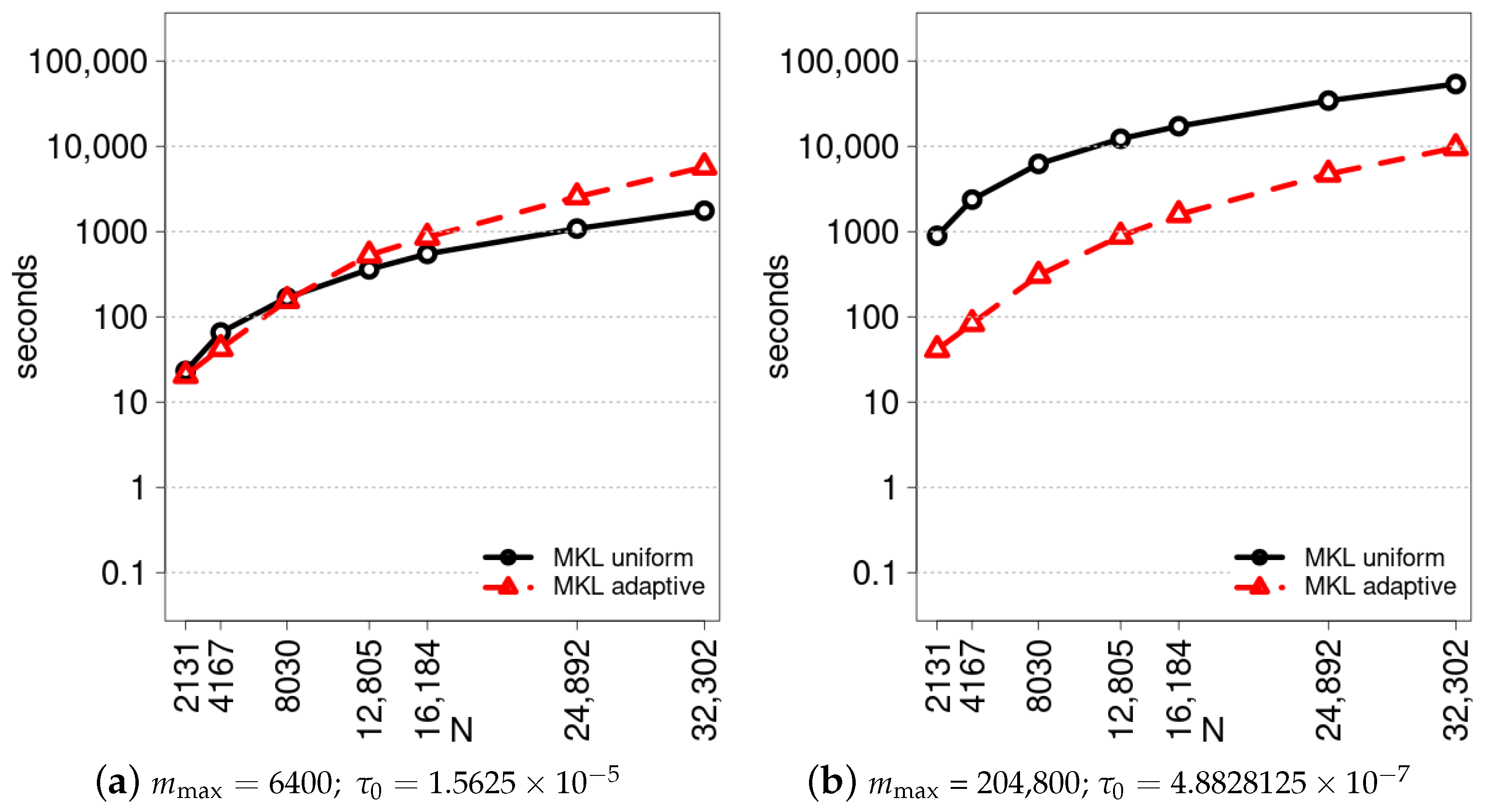
6. Comparative Analysis of Sequential Performance

Here, we analyse the performance of the adaptive scheme compared to the backward Euler algorithm with uniform time step $\tau ={\tau }_0$. Figure 2 shows the computation times of the sequential algorithms with the LU factorization solver. We see that the adaptive time stepping scheme has a clear advantage in the case of a smaller time step ${\tau }_0=4.8828125\times {10}^{-7}$. This experimental result is fully consistent with the theoretical conclusion in Section 4 that the adaptive method has better computational complexity when $m<N$. The number of steps generated by the adaptive algorithm is presented in Figure 3. We observe that although the minimum step size is reduced by two orders of magnitude, the amount of adaptive time steps is increased by only a factor of approximately two. In other words, the discussed adaptive strategy leads to a logarithmic increase in the total number of time steps with respect to ${\tau }_0$, that is, $m=O\left(\right|log{\tau }_0\left|\right)$. This explains the much better computational times of the adaptive method when ${\tau }_0$ is small enough.

Let us recall that the adaptive forward–backward Euler method developed is explicit. We do not need inner iterations to fit the error estimator. Avoiding inner iterations is an important sought-after property of the algorithm, taking into account the non-locality of the fractional diffusion and the fact that the stiffness matrix is dense.

The following Figure 4 plays a key role in the experimental proof-of-concept of the approach proposed in this paper. Here, we present a comparison of the computational times of the adaptive algorithm with LU-based and HSS-based solvers. For both variants of the minimum time step ${\tau }_0$, hierarchical compression performs much better. It should be noted that there is little difference between the results with ${\tau }_0=1.5625\times {10}^{-5}$ and ${\tau }_0=4.8828125\times {10}^{-7}$. The reason for this is that most of the steps are relatively larger, except for the locally refined ones around the jump points of $f(x,t)$. Figure 5 illustrates this behaviour of the adaptive step sizes over the entire time interval. We also see the monotonically increasing time steps in the subintervals where the right-hand side does not change. This is consistent with the evolving smoothness of the solution.

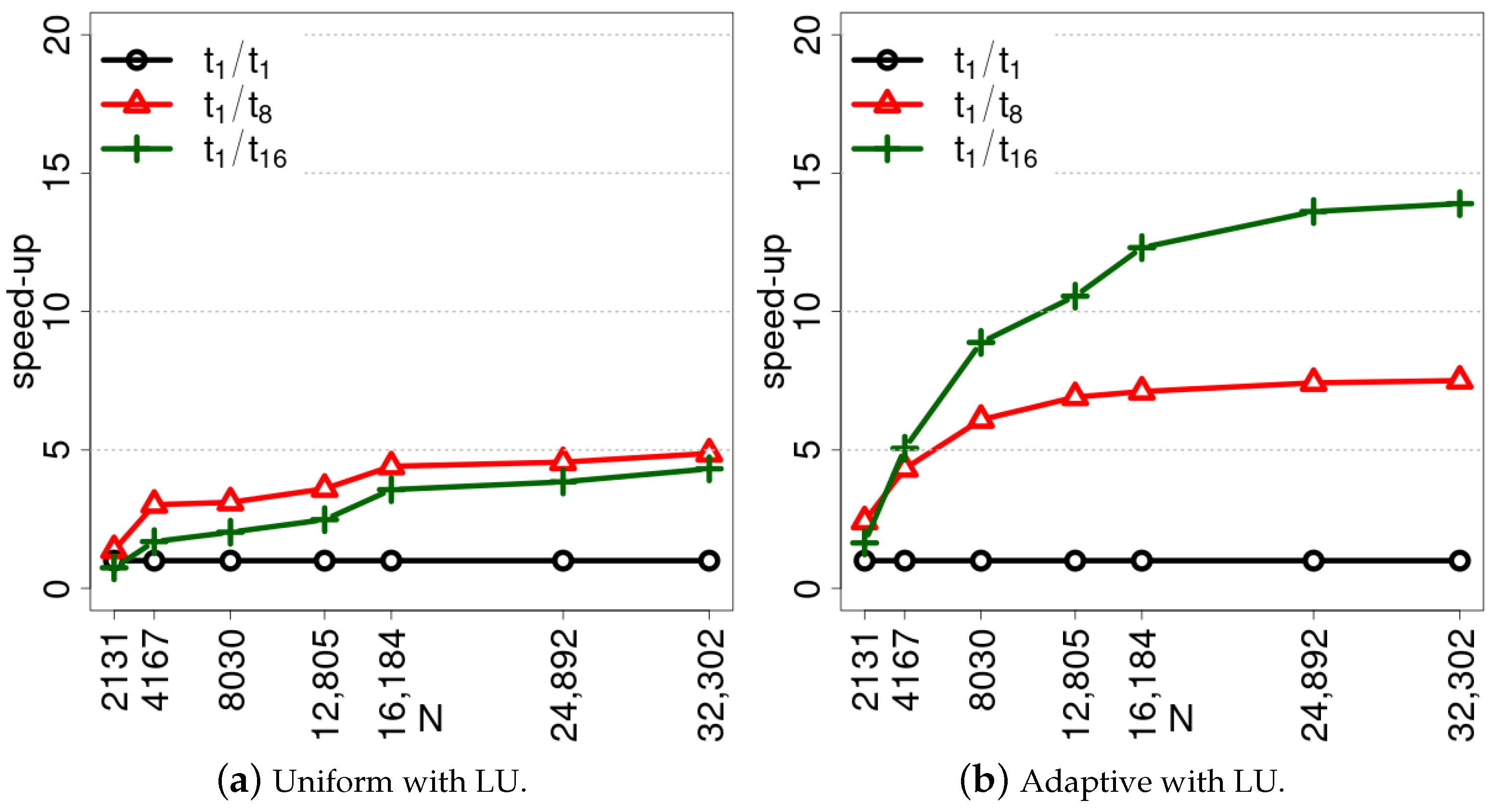
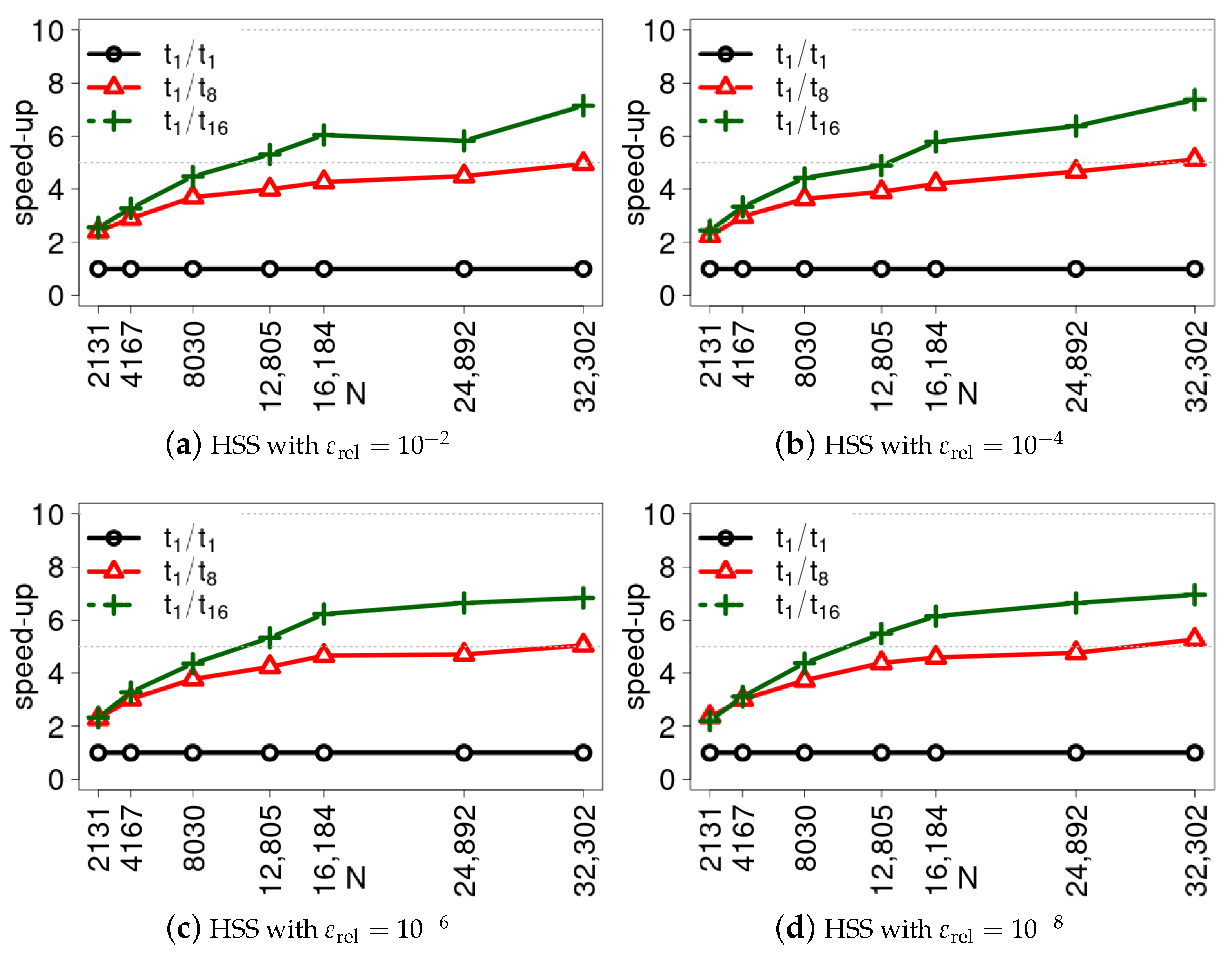
7. Parallel Scalability

For large-scale problems, the efficient implementation of computing systems with parallel architecture becomes an increasingly important issue. Solving dense linear systems with block LU-based solvers is a commonly accepted standard for measuring the performance of supercomputers. This approach is used in the well-known LINPACK TOP 500 ranking [33]. And although numerical linear algebra is the backbone of computing in general, evaluating the overall performance of a real-life problem is always a more complex task than benchmarking a single routine. Ensuring a transparent comparison, we follow the steps from Section 6 here, now analyzing the parallel performance. Let us also recall that MKL and STRUMPACK were developed as parallel software packages.

In Figure 6, we present the parallel times for the backward Euler method with a uniform time step and the adaptive forward–backward Euler time stepping scheme. The block LU-based solver from MKL is used. The tests were run on a single server with 16 threads. Similar to the sequential tests, the adaptive scheme has better times for all N values at smaller ${\tau }_0$; see the graph on the right-hand side. However, we also observe a relative improvement in parallel times in the case of ${\tau }_0=1.5625\times {10}^{-5}$. This is because the solution with the already factorized system has a lower parallel speed-up, which can be seen in Figure 7. With 16 threads, the adaptive method achieves up to ∼14 times better computation time than the sequential one, while the speed-up for the uniform time step method is only ∼5. Further details on the parallel speed-up of the LU factorization step and then of the solution step with the factorized matrix system can be found in [22].

In Figure 8, we present the parallel times with LU factorization and HSS-compression-based solvers for the adaptive method. For all experiments, HSS compression outperforms LU factorization. This means that the stiffness matrix obtained from the FEM discretization of the fractional Laplacian is suitable for hierarchical semi-separable compression. Overall, the adaptive algorithm with the HSS compression solver has a lower parallel speed-up of ∼6 (see Figure 9) compared to the adaptive method with LU factorization (see Figure 7), but its better performance is due to the substantially lower computational complexity.

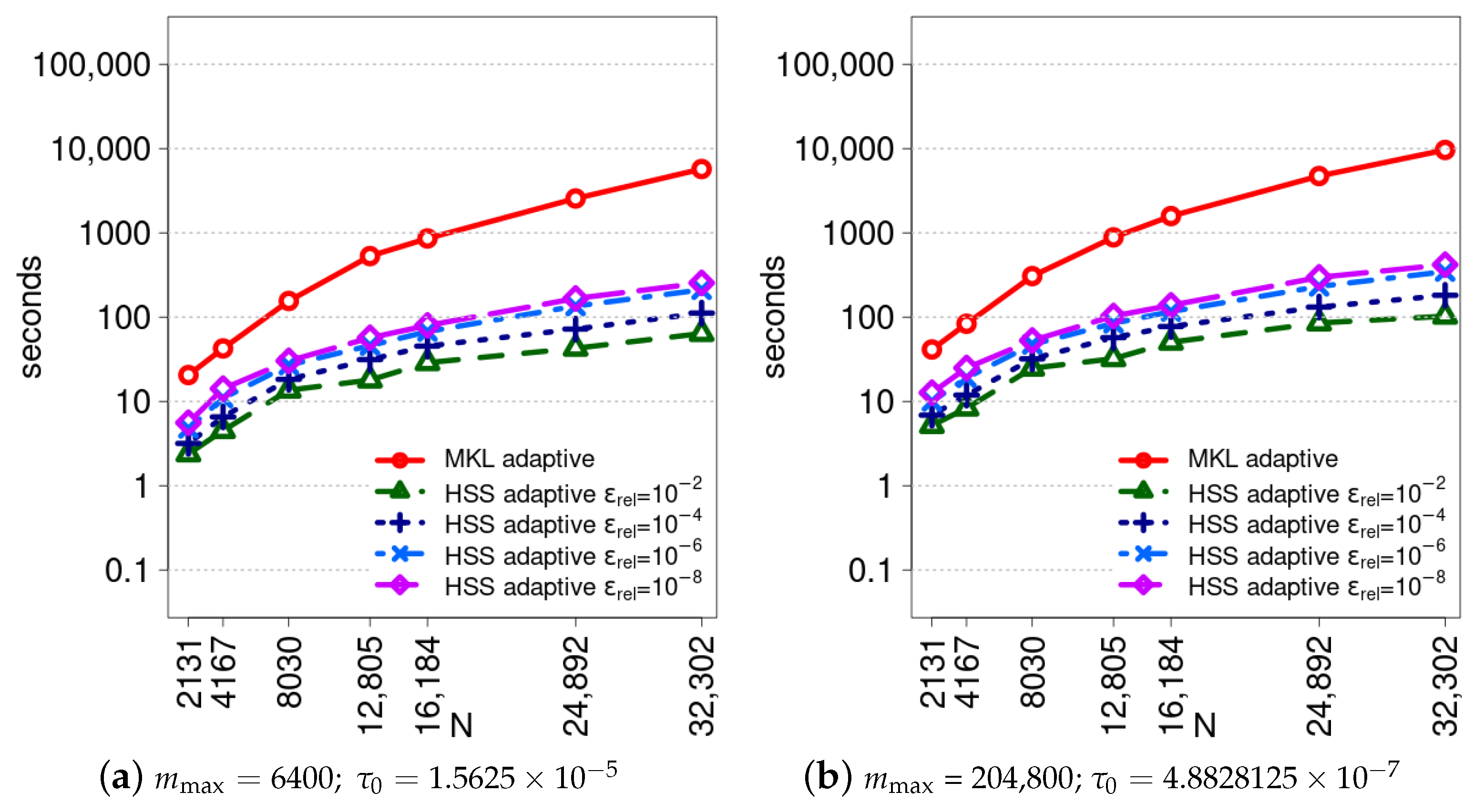
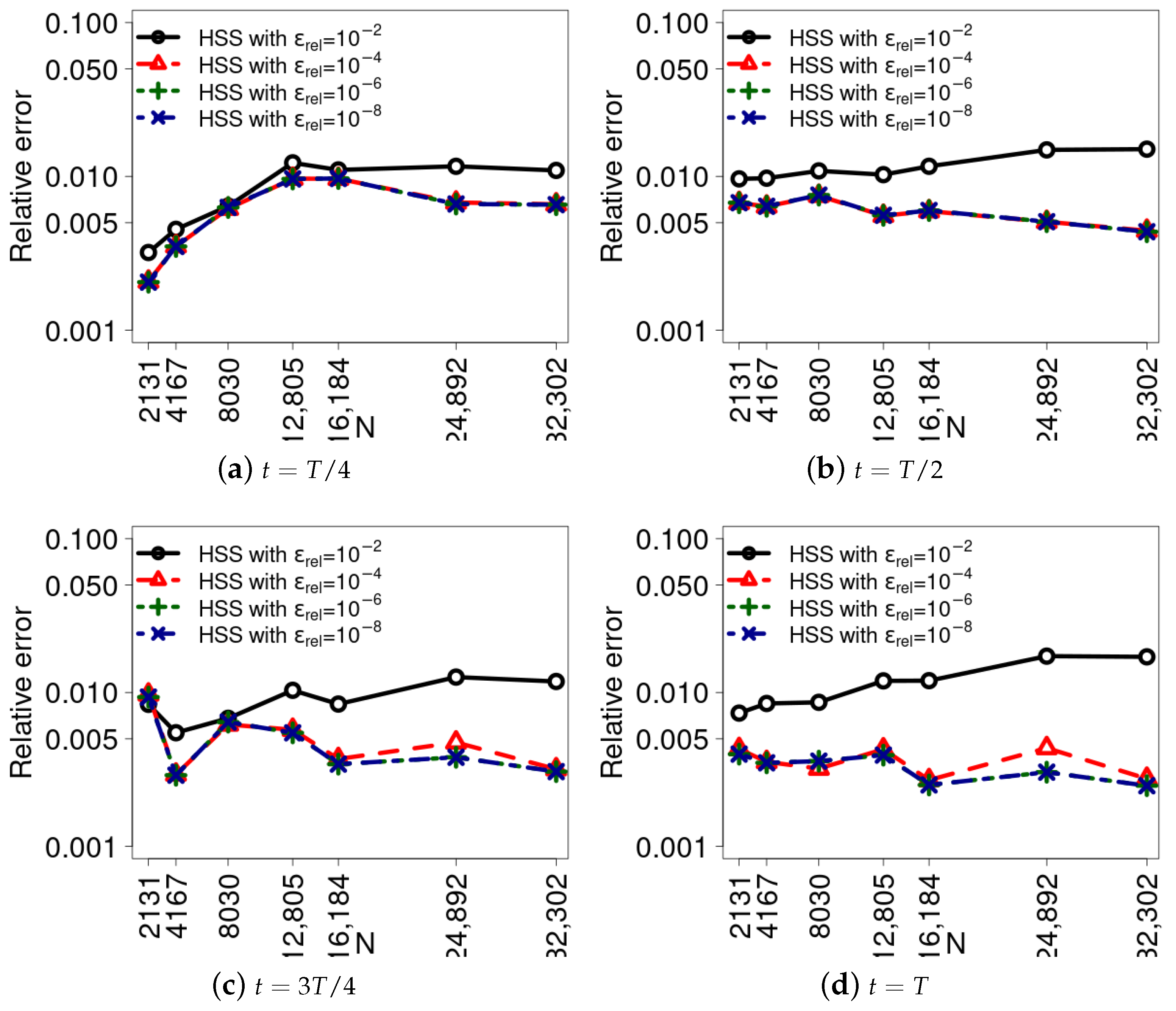
8. Analysis of Relative Errors of the HSS Compression Solver

The hierarchical semi-separable compressed representation of matrices is approximate. In the numerical experiments, we presented computational times and speed-up with four values of the relative threshold that is used in the compression algorithm implemented in the STRUMPACK package. In Figure 10, we show the relative errors with respect to the reference solution obtained by the uniform method with LU factorization. For the backward Euler method with a uniform time step, this relative error is of the order ${\epsilon }_{\mathrm{rel}}$ (see [20]). Here, we show the calculated values of $R_j$ at the time points $T/4$, $T/2$, $3T/4$, and T, recalling that $T=0.1$. What we see is that for the adaptive method, decreasing the relative threshold after ${10}^{-4}$ does not improve the relative error. And this is exactly what we should expect from the numerical tests, where the desired accuracy parameter was set to $\delta =0.01$.

9. Discussion

In the case of standard (local) differential equations, there have been many years of successful work on the development of numerical methods for parabolic problems. In particular, the stiffness and mass matrices are sparse and positive definite if the FEM is applied to discretization in space. Thus, explicit methods have an optimal complexity with respect to N, with an analogous result obtained for implicit methods if fast (e.g., multigrid or multilevel) PCG iterative solvers are used. The methods and algorithms discussed here show how the challenges change substantially when moving from local to non-local problems.

Complex solutions are integrated to ensure the computational efficiency of the developed method. A successful combination of the near-optimal unconditionally stable adaptive backward–forward Euler scheme with the upgraded HSS compression-based solver for the diagonally perturbed stiffness matrices that appear in transient systems is achieved. In addition, although recursive by definition, HSS compression and its implementation in the STRUMPACK software package show promising parallel scalability within the discussed composite algorithm.

The numerical experiments show a very good agreement with the theoretical results, thus proving the concept of the applied research methodology. We note the following conclusions: the advantages of the adaptive scheme increase as the minimum time step decreases; the HSS compression-based solver outperforms the LU factorization; the overall accuracy is effectively controlled by the parameters of the adaptive scheme and the HSS compression.

10. Conclusions

In conclusion, the main contribution of the paper is determined by the development, analysis and implementation of a new highly efficient numerical method and algorithms for parabolic diffusion problems with a fractional Laplacian in space. The theoretical results, including, in particular, computational complexity estimates and scalability analyses, are clearly confirmed by the sequential and parallel numerical tests presented. The adaptive backward–forward Euler scheme optimizes computational complexity by avoiding the need for prior assumptions about the regularity of the solution. The algorithm essentially uses the fact that the time derivative is standard (local). For this reason, the concept of an adaptive time stepping will need extensive further development in the case of fractional (nonlocal) diffusion in time.

The progress made in this paper poses new challenges and creates new opportunities for future research in the development of numerical methods for time-dependent fractional diffusion problems in space. In this context, the following topics are on our short-term priority list: adaptive higher-order schemes; adaptive time steps for spectral fractional diffusion; and combining adaptive time stepping with local mesh refinement and hp-FEM in space.

The present investigations can naturally be extended to more general equations that include a fractional power of the diffusion operator (e.g., the Laplacian). This applies, for example, to the case of reaction and/or convection-type terms, where the monotonicity conditions of the schemes may be of particular interest along with stability issues.

The nonlinear case is a separate topic of great scientific value and practical importance. Here, there are very wide possibilities for implementing and upgrading the adaptive time-stepping methods and algorithms. Such an example is the time-dependent fractional in a space diffusion–reaction system of equations coupled by nonlinear reaction operators [34].

References

1. Binder, K.; Bennemann, C.; Baschnagel, J.; Paul, W. Anomalous diffusion of polymers in supercooled melts near the glass transition. In Anomalous Diffusion from Basics to Applications; Pękalski, A., Sznajd-Weron, K., Eds.; Springer: Berlin/Heidelberg, Germany, 1999; pp. 124–139. [Google Scholar]
2. Langlands, T.; Henry, B.; Wearne, S. Fractional Cable Equation Models for Anomalous Electrodiffusion in Nerve Cells: Finite Domain Solutions. SIAM J. Appl. Math. 2011, 71, 1168–1203. [Google Scholar] [CrossRef]
3. Taitelbaum, H. Diagnosis using photon diffusion: From brain oxygenation to the fat of the atlantic salmon. In Anomalous Diffusion from Basics to Applications; Pękalski, A., Sznajd-Weron, K., Eds.; Springer: Berlin/Heidelberg, Germany, 1999; pp. 160–174. [Google Scholar]
4. Rosasco, L.; Belkin, M.; Vito, E.D. On Learning with Integral Operators. J. Mach. Learn. Res. 2010, 11, 905–934. [Google Scholar]
5. Chaturapruek, S.; Breslau, J.; Yazdi, D.; Kolokolnikov, T.; McCalla, S. Crime modeling with Lèvy flights. SIAM J. Appl. Math. 2013, 73, 1703–1720. [Google Scholar] [CrossRef]
6. Sun, H.; Zhang, Y.; Baleanu, D.; Chen, W.; Chen, Y. A new collection of real world applications of fractional calculus in science and engineering. Commun. Nonlinear Sci. Numer. Simul. 2018, 64, 213–231. [Google Scholar] [CrossRef]
7. Kwaśnicki, M. Ten equivalent definitions of the fractional laplace operator. Fract. Calc. Appl. Anal. 2017, 20, 7–51. [Google Scholar] [CrossRef]
8. Lischke, A.; Pang, G.; Gulian, M.; Song, F.; Glusa, C.; Zheng, X.; Mao, Z.; Cai, W.; Meerschaert, M.M.; Ainsworth, M.; et al. What is the fractional Laplacian? A comparative review with new results. J. Comput. Phys. 2020, 404, 109009. [Google Scholar] [CrossRef]
9. Harizanov, S.; Margenov, S.; Popivanov, N. Spectral Fractional Laplacian with Inhomogeneous Dirichlet Data: Questions, Problems, Solutions. In Advanced Computing in Industrial Mathematics; Georgiev, I., Kostadinov, H., Lilkova, E., Eds.; Springer: Cham, Switzerland, 2021; pp. 123–138. [Google Scholar] [CrossRef]
10. Bonito, A.; Lei, W.; Pasciak, J.E. The approximation of parabolic equations involving fractional powers of elliptic operators. J. Comput. Appl. Math. 2017, 315, 32–48. [Google Scholar] [CrossRef]
11. Markus Melenk, J.; Rieder, A. An exponentially convergent discretization for space–time fractional parabolic equations using hp-FEM. IMA J. Numer. Anal. 2022, 43, 2352–2376. [Google Scholar] [CrossRef]
12. Nochetto, R.H.; Otárola, E.; Salgado, A.J. A PDE Approach to Space-Time Fractional Parabolic Problems. SIAM J. Numer. Anal. 2016, 54, 848–873. [Google Scholar] [CrossRef]
13. Vabishchevich, P.N. Splitting schemes for non-stationary problems with a rational approximation for fractional powers of the operator. Appl. Numer. Math. 2021, 165, 414–430. [Google Scholar] [CrossRef]
14. Vabishchevich, P.N. Numerical Solution of Non-stationary Problems for a Space-Fractional Diffusion Equation. Fract. Calc. Appl. Anal. 2016, 19, 116–139. [Google Scholar] [CrossRef]
15. Čiegis, R.; Starikovičius, V.; Suboč, O.; Čiegis, R. On Construction of Partially Dimension-Reduced Approximations for Nonstationary Nonlocal Problems of a Parabolic Type. Mathematics 2023, 11, 1984. [Google Scholar] [CrossRef]
16. Danczul, T.; Hofreither, C.; Schöberl, J. A unified rational Krylov method for elliptic and parabolic fractional diffusion problems. Numer. Linear Algebra Appl. 2023, 30, e2488. [Google Scholar] [CrossRef]
17. Khristenko, U.; Wohlmuth, B. Solving time-fractional differential equations via rational approximation. IMA J. Numer. Anal. 2022, 43, 1263–1290. [Google Scholar] [CrossRef]
18. Yang, Y.; Huang, J. Double fast algorithm for solving time-space fractional diffusion problems with spectral fractional Laplacian. Appl. Math. Comput. 2024, 475, 128715. [Google Scholar] [CrossRef]
19. Acosta, G.; Bersetche, F.M.; Borthagaray, J.P. Finite Element Approximations for Fractional Evolution Problems. Fract. Calc. Appl. Anal. 2019, 22, 767–794. [Google Scholar] [CrossRef]
20. Slavchev, D.; Margenov, S. Performance Study of Hierarchical Semi-separable Compression Solver for Parabolic Problems with Space-Fractional Diffusion. In Large-Scale Scientific Computing; Lirkov, I., Margenov, S., Eds.; Springer: Cham, Switzerland, 2022; pp. 71–80. [Google Scholar]
21. Acosta, G.; Borthagaray, J. A Fractional Laplace Equation: Regularity of Solutions and Finite Element Approximations. SIAM J. Numer. Anal. 2017, 55, 472–495. [Google Scholar] [CrossRef]
22. Slavchev, D.; Margenov, S. On the Application of a Hierarchically Semi-separable Compression for Space-Fractional Parabolic Problems with Varying Time Steps. In Numerical Methods and Applications; Georgiev, I., Datcheva, M., Georgiev, K., Nikolov, G., Eds.; Springer: Cham, Switzerland, 2023; pp. 289–301. [Google Scholar]
23. Blaheta, R.; Byczanski, P.; Kohut, R.; Starỳ, J. Algorithms for Parallel Fem Modelling of Thermo-Mechanical Phenomena Arising from the Disposal of the Spent Nuclear Fuel. In Elsevier Geo-Engineering Book Series; Elsevier: Amsterdam, The Netherlands, 2004; Volume 2, pp. 395–400. [Google Scholar]
24. Georgiev, K.; Kosturski, N.; Margenov, S.; Starỳ, J. On adaptive time stepping for large-scale parabolic problems: Computer simulation of heat and mass transfer in vacuum freeze-drying. J. Comput. Appl. Math. 2009, 226, 268–274. [Google Scholar] [CrossRef]
25. Vabishchevich, P.N.; Vasil’ev, A.O. Time step selection for the numerical solution of boundary value problems for parabolic equations. Comput. Math. Math. Phys. 2017, 57, 843–853. [Google Scholar] [CrossRef]
26. Hackbusch, W. A Sparse Matrix Arithmetic Based on H-Matrices. Part I: Introduction to H-Matrices. Computing 1999, 62, 89–108. [Google Scholar] [CrossRef]
27. Hackbusch, W.; Grasedyck, L.; Börm, S. An introduction to hierarchical matrices. Math. Bohem. 2002, 127, 229–241. [Google Scholar] [CrossRef]
28. Martinsson, P.G. A Fast Randomized Algorithm for Computing a Hierarchically Semiseparable Representation of a Matrix. SIAM J. Matrix Anal. Appl. 2011, 32, 1251–1274. [Google Scholar] [CrossRef]
29. Xia, J.; Chandrasekaran, S.; Gu, M.; Li, X.S. Fast algorithms for hierarchically semiseparable matrices. Numer. Lin. Alg. Appl. 2010, 17, 953–976. [Google Scholar] [CrossRef]
30. Rouet, F.H.; Li, X.; Ghysels, P.; Napov, A. A Distributed-Memory Package for Dense Hierarchically Semi-Separable Matrix Computations Using Randomization. ACM Trans. Math. Softw. 2016, 42, 1–35. [Google Scholar] [CrossRef]
31. Slavchev, D.; Margenov, S.; Georgiev, I. On the application of recursive bisection and nested dissection reorderings for solving fractional diffusion problems using HSS compression. AIP Conf. Proc. 2020, 2302, 120008. [Google Scholar] [CrossRef]
32. Rebrova, E.; Chávez, G.; Liu, Y.; Ghysels, P.; Li, X.S. A Study of Clustering Techniques and Hierarchical Matrix Formats for Kernel Ridge Regression. In Proceedings of the 2018 IEEE International Parallel and Distributed Processing Symposium Workshops (IPDPSW), Vancouver, BC, Canada, 21–25 May 2018; pp. 883–892. [Google Scholar] [CrossRef]
33. Dongarra, J.J.; Luszczek, P.; Petitet, A. The LINPACK Benchmark: Past, present and future. Concurr. Comput. Pract. Exp. 2003, 15, 803–820. [Google Scholar] [CrossRef]
34. Georgiev, K.; Margenov, S. Numerical Methods for Fractional Diffusion-Reaction Problems Based on Operator Splitting and BURA. In Advanced Computing in Industrial Mathematics; Georgiev, I., Kostadinov, H., Lilkova, E., Eds.; Springer: Cham, Switzerland, 2023; pp. 73–84. [Google Scholar]
Figure 1. Backward Euler method with uniform time step: reduction in relative error R j versus decrease in τ for N = 2131.
Algorithms 17 00453 g001
Figure 2. Sequential computational times of the uniform and adaptive schemes with LU factorization from the MKL package.
Algorithms 17 00453 g002
Figure 3. Number of adaptive steps used for both minimum step sizes.
Algorithms 17 00453 g003
Figure 4. Sequential computational times of adaptive scheme with LU factorization and HSS compression.
Algorithms 17 00453 g004
Figure 5. Adaptive time step size over the whole time interval for N = 2131 and τ 0 = 1.5625 × 10 5 with LU solver.
Algorithms 17 00453 g005
Figure 6. Parallel computational times of the uniform and adaptive LU solvers from MKL.
Algorithms 17 00453 g006
Figure 7. Parallel speed-up (parallel time divided by sequential time) of the uniform and adaptive methods with an LU factorization-based solver. The speed-up is calculated for τ 0 = 4.8828125 × 10 7 experiments but is similar to the other value of τ 0 .
Algorithms 17 00453 g007
Figure 8. Parallel times of the uniform and adaptive schemes with HSS compression and ULV-like factorization from the STRUMPACK package.
Algorithms 17 00453 g008
Figure 9. Parallel speed-up of the HSS compression and ULV-like factorization-based solver for the adaptive algorithm.
Algorithms 17 00453 g009
Figure 10. Relative errors of the solution with τ 0 = 4.8828125 × 10 7 of the adaptive method with HSS compression in relation to the uniform method with LU factorization for ε rel = 10 2 , 10 4 , 10 6 , 10 8 .
Algorithms 17 00453 g010
Disclaimer/Publisher’s Note: The statements, opinions and data contained in all publications are solely those of the individual author(s) and contributor(s) and not of MDPI and/or the editor(s). MDPI and/or the editor(s) disclaim responsibility for any injury to people or property resulting from any ideas, methods, instructions or products referred to in the content.