
Root Cause Attribution of Delivery Risks via Causal Discovery with Reinforcement Learning


Abstract
1. Introduction
Existing Works in Supply Chain on Delivery Risk
2. Methodology
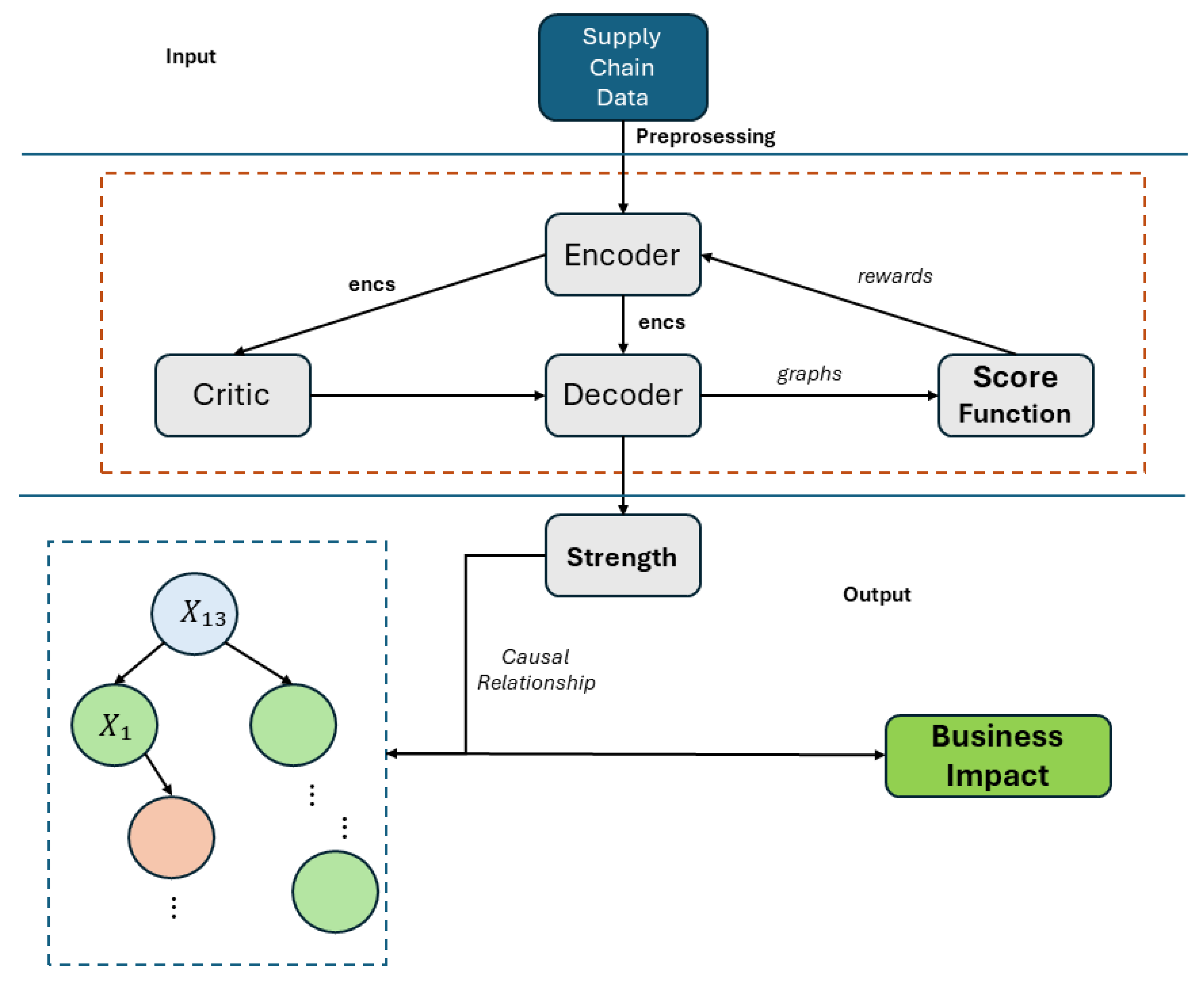
The Proposed Method
| Algorithm 1 Causal Discovery with RL for Late Delivery Risk |
|
3. Experiments
3.1. Experimental Data
3.1.1. DataCo Global
3.1.2. Explanatory Data Analysis
3.2. Experimental Analysis
4. Discussion and Business Impact
- Improving Shipping Strategies: Our analysis revealed that the choice of shipping mode () has a direct and significant impact on actual shipping days (), which, in turn, greatly influences the risk of late deliveries (). The causal strength of 9.24 between shipping mode and actual shipping days highlights the critical role of selecting optimal shipping methods to minimize delays. By leveraging our causal discovery approach, businesses can optimize their shipping strategies, prioritizing methods that reduce delivery times and thus mitigate late delivery risks. This can lead to improved customer satisfaction and reduced operational costs.
- Enhancing Delivery Status Monitoring: The direct relationship between delivery status () and late delivery risk (), with a causal strength of 10.66, underscores the importance of real-time monitoring and management of delivery processes. Our method allows businesses to identify the statuses most predictive of delays, facilitating targeted interventions to address bottlenecks. By improving the monitoring of delivery statuses, companies can proactively reduce late deliveries, enhancing supply chain efficiency and providing a more reliable service.
- Strategic Pricing and Inventory Decisions: Beyond delivery concerns, our analysis found that ‘Order Item Profit Ratio’ () and ‘Order Item Product Price’ () influence ‘Benefit per Order’ (). While not directly related to late delivery risks, these findings are crucial for profitability. The causal strength of 2.20 for the profit ratio suggests that optimizing profit margins is key to maximizing order-level benefits. By applying our causal discovery approach, businesses can refine their pricing strategies and inventory decisions to enhance profitability, leading to more informed decision-making and improved financial performance across the supply chain.
5. Conclusions and Future Work
Author Contributions
Funding
Informed Consent Statement
Data Availability Statement
Conflicts of Interest
Abbreviations
| IIE | Inverse information entropy |
| BIC | Bayesian information criterion |
| DoS | Days of shipment |
| RL | Reinforcement Learning |
| EDA | Exploratory data analysis |
Appendix A. Data Description

| Variable | Description |
|---|---|
| Type | Type of transaction made |
| Days for shipping (real) | Actual shipping days of the purchased product |
| Days for shipment (scheduled) | Days of scheduled delivery of the purchased product |
| Benefit per order | Earnings per order placed |
| Sales per customer | Total sales per customer made per customer |
| Delivery Status | Delivery status of orders: Advance shipping or not |
| Late_delivery_risk | Categorical variable that indicates if sending the product would cause a late delivery |
| Customer Segment | Business segment of the customer |
| Latitude | Latitude coordinates of the purchase |
| Longitude | Longitude coordinates of the purchase |
| Order Item Discount Rate | Order item discount percentage |
| Order Item Product Price | Price of products without discount |
| Order Item Profit Ratio | Order Item Profit Ratio |
| Order Item Quantity | Number of products per order |
| Order Status | Order Status: COMPLETE, PENDING, CLOSED, etc. |
| Shipping Mode | The following shipping modes are presented: First Class, Second Class, Same Day, etc. |
References
- Ketchen Jr, D.J.; Rebarick, W.; Hult, G.T.M.; Meyer, D. Best value supply chains: A key competitive weapon for the 21st century. Bus. Horiz. 2008, 51, 235–243. [Google Scholar] [CrossRef]
- Singh, J.; Singh, P. Why Is Apple’s Supply Chain Management The Best In The World? Int. J. Humanit. Manag. 2015, II, 1. [Google Scholar]
- Ivanov, D. Predicting the impact of the COVID-19 pandemic on global supply chains: A simulation-based analysis on the case of China. Transp. Res. Part Logist. Transp. Rev. 2020, 136, 101922. [Google Scholar] [CrossRef]
- Park, J.; Hong, S.Y. Just-in-time production systems in the aftermath of a disaster: The 2011 Japanese earthquake and tsunami. Bus. Horiz. 2013, 56, 75–85. [Google Scholar] [CrossRef]
- Blanchard, D. Supply Chain Management: Best Practices; John Wiley & Sons: Hoboken, NJ, USA, 2021. [Google Scholar]
- Neuberg, J. Causality and correlation: Pitfalls of traditional statistical methods. Stat. Sci. 2003, 18, 465–475. [Google Scholar]
- Mao, H.; Görg, H. Friends like this: The impact of the US–China trade war on global value chains. World Econ. 2020, 43, 1776–1791. [Google Scholar] [CrossRef]
- Christopher, M.; Peck, H. Building the resilient supply chain. Int. J. Logist. Manag. 2004, 15, 1–13. [Google Scholar] [CrossRef]
- Peters, J.; Janzing, D.; Schölkopf, B. Elements of Causal Inference: Foundations and Learning Algorithms; The MIT Press: Cambridge, MA, USA, 2017. [Google Scholar]
- Zhu, S.; Ng, I.; Chen, Z. Causal discovery with reinforcement learning. arXiv 2019, arXiv:1906.04477. [Google Scholar]
- Le, T.D.; Hoang, T.; Li, J.; Liu, L.; Liu, H.; Hu, S. A fast PC algorithm for high dimensional causal discovery with multi-core PCs. IEEE ACM Trans. Comput. Biol. Bioinform. 2016, 16, 1483–1495. [Google Scholar] [CrossRef]
- He, Z.; Deng, S.; Xu, X.; Huang, J.Z. A fast greedy algorithm for outlier mining. In Proceedings of the Advances in Knowledge Discovery and Data Mining: 10th Pacific-Asia Conference, PAKDD 2006, Singapore, 9–12 April 2006; Proceedings 10. Springer: Berlin/Heidelberg, Germany, 2006; pp. 567–576. [Google Scholar]
- Bicer, I.; Seifert, R.W. Optimal dynamic order scheduling under capacity constraints given demand-forecast evolution. Prod. Oper. Manag. 2017, 26, 2266–2286. [Google Scholar] [CrossRef]
- Chen, H.; Zuo, L.; Wu, C.; Wang, L.; Diao, F.; Chen, J.; Huang, Y. Optimizing detailed schedules of a multiproduct pipeline by a monolithic MILP formulation. J. Pet. Sci. Eng. 2017, 159, 148–163. [Google Scholar] [CrossRef]
- Bushuev, M.A.; Filatova, E.A. Delivery strategy improvement for e-commerce supply chain. J. Ind. Eng. Manag. 2018, 11, 50–64. [Google Scholar]
- Shao, X.; Tang, W. Production and delivery scheduling with deteriorating jobs and time-dependent learning effects. J. Oper. Res. Soc. 2018, 69, 108–121. [Google Scholar]
- Chong, A.Y.; Ch’ng, E.; Liu, M.J.; Li, B. Predicting late delivery risk using artificial neural networks. Expert Syst. Appl. 2018, 88, 1–10. [Google Scholar]
- Ryu, S.; Kang, K.; Lee, H. Predicting delivery delays in supply chain management using machine learning. J. Manuf. Syst. 2019, 50, 1–14. [Google Scholar]
- Lim, J.H.; Park, K.Y. Predicting delivery risk using ensemble learning techniques. IEEE Access 2019, 7, 156634–156642. [Google Scholar]
- Wang, S.; Zeng, J. Supply chain disruption risk management using machine learning. J. Manuf. Syst. 2019, 51, 195–206. [Google Scholar]
- Bo, S.; Zhang, Y.; Huang, J.; Liu, S.; Chen, Z.; Li, Z. Attention Mechanism and Context Modeling System for Text Mining Machine Translation. arXiv 2024, arXiv:2408.04216. [Google Scholar]
- Verma, S.; Gangele, V. Supply chain risk management using deep learning techniques. Int. J. Comput. Appl. 2019, 178, 8–12. [Google Scholar]
- Cruijssen, F.; Dullaert, W. Enhancing supply chain resilience through supply chain collaboration: An optimization perspective. Transp. Res. Part Logist. Transp. Rev. 2019, 122, 14–26. [Google Scholar]
- Mourtzis, D.; Vlachou, E. Real-time monitoring and control in manufacturing: The role of digital twin and industry 4.0. Procedia CIRP 2019, 81, 467–472. [Google Scholar]
- Mishra, A.; Kumar, S. Smart supply chain management: A review and future research directions. J. Clean. Prod. 2020, 273, 123091. [Google Scholar]
- Zhou, K.; Dai, C. Supply chain risk prediction and management using deep reinforcement learning. J. Artif. Intell. Res. 2018, 62, 575–589. [Google Scholar]
- Lee, I.; Lee, K. The Internet of Things (IoT): Applications, investments, and challenges for enterprises. Bus. Horiz. 2018, 61, 577–590. [Google Scholar] [CrossRef]
- Janjua, M.B.; Kausar, F. Real-time monitoring of delivery risks in supply chain using IoT and big data. J. Supply Chain. Manag. 2019, 55, 30–45. [Google Scholar]
- Lin, H.; Chen, C.H. Real-time risk management in smart manufacturing systems: A case study on IoT-enabled supply chain. J. Intell. Manuf. 2020, 31, 689–701. [Google Scholar]
- Liu, C.; Yu, L. Internet of Things for improving supply chain risk management: A systematic review. Int. J. Prod. Res. 2020, 58, 2954–2975. [Google Scholar]
- Hoyer, P.; Janzing, D.; Mooij, J.M.; Peters, J.; Schölkopf, B. Nonlinear causal discovery with additive noise models. In Proceedings of the Advances in Neural Information Processing Systems 21, Proceedings of the Twenty-Second Annual Conference on Neural Information Processing Systems, Vancouver, BC, Canada, 8–11 December 2008. [Google Scholar]
- Peters, J.; Mooij, J.M.; Janzing, D.; Schölkopf, B. Causal Discovery with Continuous Additive Noise Models. J. Mach. Learn. Res. 2014, 15, 2009–2053. [Google Scholar]
- Mu, G.; Chen, Q.; Liu, H.; An, J.; Wang, C. The inverse information entropy causal reasoning method to reveal causality in power system operation data. Chin. J. Electr. Eng. 2022, 42, 5406–5417. [Google Scholar]
- Vaswani, A.; Shazeer, N.; Parmar, N.; Uszkoreit, J.; Jones, L.; Gomez, A.N.; Kaiser, L.; Polosukhin, I. Attention is all you need. In Proceedings of the Advances in Neural Information Processing Systems 30: Annual Conference on Neural Information Processing Systems 2017, Long Beach, CA, USA, 4–9 December 2017. [Google Scholar]
- He, K.; Zhang, X.; Ren, S.; Sun, J. Deep residual learning for image recognition. In Proceedings of the IEEE Conference on Computer Vision and Pattern Recognition, Las Vegas, NV, USA, 27–30 June 2016; pp. 770–778. [Google Scholar]
- Zheng, X.; Aragam, B.; Ravikumar, P.K.; Xing, E.P. Dags with no tears: Continuous optimization for structure learning. In Proceedings of the Advances in Neural Information Processing Systems 31: Annual Conference on Neural Information Processing Systems 2018, NeurIPS 2018, Montreal, QC, Canada, 3–8 December 2018. [Google Scholar]
- Daniusis, P.; Janzing, D.; Mooij, J.; Zscheischler, J.; Steudel, B.; Zhang, K.; Schölkopf, B. Inferring deterministic causal relations. arXiv 2012, arXiv:1203.3475. [Google Scholar]
- Kraskov, A.; Stögbauer, H.; Grassberger, P. Estimating mutual information. Phys. Rev. Stat. Nonlinear Soft Matter Phys. 2004, 69, 066138. [Google Scholar] [CrossRef] [PubMed]
- Bramer, M.; Heath, T. Data Mining for Advanced Analytics: Techniques for Risk Assessment and Decision-Making; Springer: Berlin/Heidelberg, Germany, 2016. [Google Scholar]


| Article | Existing Methods | Results |
|---|---|---|
| [13] | Optimized Production Processes | Mitigated delays at the production stage |
| [14] | Optimizing delivery strategies | Reduced delivery delays post-risk materialization |
| [15] | Enhanced delivery strategies | Improved on-time delivery rate by optimizing routes |
| [17] | Machine Learning (Random Forest) | Improved accuracy in predicting delivery delays |
| [19] | Support Vector Machines | Identified key delay patterns in historical data |
| [21] | Clustering with Attention | Higher predictive accuracy for identifying delayed shipments |
| [23] | Optimization Algorithms | Adjusted inventory levels and routing plans to mitigate delays |
| [24] | Real-Time Adjustment (IoT) | Enabled dynamic responses to real-time risks |
| [28] | IoT-enabled Supply Chain Management | Improved response time to detected delivery risks |
| [30] | IoT and Predictive Analytics | Detected anomalies and delayed shipments using sensor data |
| Parameter | Value | Description |
|---|---|---|
| Learning Rate | 0.001 | Controls the size of the step taken in each iteration during gradient descent. Chosen to ensure stable convergence without overshooting. |
| Epochs | 500 | Number of iterations over the entire dataset during training. Selected based on performance stabilization after cross-validation. |
| Batch Size | 64 | Number of samples processed before the model updates. A moderate size chosen for memory efficiency and gradient accuracy. |
| Optimizer | Adam | Adam optimizer dynamically adjusts learning rates, suited for handling sparse gradients and noisy data in supply chains. |
| Regularization (L2) | Prevents overfitting by penalizing large weights. Regularization factor tuned for balance between complexity and generalization. | |
| Dropout Rate | 0.2 | Reduces overfitting. A value of 20% chosen based on experimentation for improved generalization. |
| Reward Function Parameters | , | Two hyperparameters for reward function: controls the causal reward weight, and is a penalty factor for weak causal links. |
| Causal Strength Threshold | 0.05 | Threshold set to filter out weaker causal links, ensuring only significant relationships are included in the causal graph. |
| Denotation | Variable | Denotation | Variable |
|---|---|---|---|
| Type | Latitude | ||
| Days for shipping (real) | Longitude | ||
| Days for shipment (scheduled) | Order Item Discount Rate | ||
| Benefit per order | Order Item Product Price | ||
| Sales per customer | Order Item Profit Ratio | ||
| Delivery Status | Order Item Quantity | ||
| Late_delivery_risk | Order Status | ||
| Customer Segment | Shipping Mode |
Disclaimer/Publisher’s Note: The statements, opinions and data contained in all publications are solely those of the individual author(s) and contributor(s) and not of MDPI and/or the editor(s). MDPI and/or the editor(s) disclaim responsibility for any injury to people or property resulting from any ideas, methods, instructions or products referred to in the content. |
© 2024 by the authors. Licensee MDPI, Basel, Switzerland. This article is an open access article distributed under the terms and conditions of the Creative Commons Attribution (CC BY) license (https://creativecommons.org/licenses/by/4.0/).
Share and Cite
Bo, S.; Xiao, M. Root Cause Attribution of Delivery Risks via Causal Discovery with Reinforcement Learning. Algorithms 2024, 17, 498. https://doi.org/10.3390/a17110498
Bo S, Xiao M. Root Cause Attribution of Delivery Risks via Causal Discovery with Reinforcement Learning. Algorithms. 2024; 17(11):498. https://doi.org/10.3390/a17110498
Chicago/Turabian StyleBo, Shi, and Minheng Xiao. 2024. "Root Cause Attribution of Delivery Risks via Causal Discovery with Reinforcement Learning" Algorithms 17, no. 11: 498. https://doi.org/10.3390/a17110498
APA StyleBo, S., & Xiao, M. (2024). Root Cause Attribution of Delivery Risks via Causal Discovery with Reinforcement Learning. Algorithms, 17(11), 498. https://doi.org/10.3390/a17110498