Improved Brain Storm Optimization Algorithm Based on Flock Decision Mutation Strategy

Abstract

To tackle the problem of the brain storm optimization (BSO) algorithm’s suboptimal capability for avoiding local optima, which contributes to its inadequate optimization precision, we developed a flock decision mutation approach that substantially enhances the efficacy of the BSO algorithm. Furthermore, to solve the problem of insufficient BSO algorithm population diversity, we introduced a strategy that utilizes the good point set to enhance the initial population’s quality. Simultaneously, we substituted the K-means clustering approach with spectral clustering to improve the clustering accuracy of the algorithm. This work introduced an enhanced version of the brain storm optimization algorithm founded on a flock decision mutation strategy (FDIBSO). The improved algorithm was compared against contemporary leading algorithms through the CEC2018. The experimental section additionally employs the AUV intelligence evaluation as an application case. It addresses the combined weight model under various dimensional settings to substantiate the efficacy of the FDIBSO algorithm further. The findings indicate that FDIBSO surpasses BSO and other enhanced algorithms for addressing intricate optimization challenges.

1. Introduction

Autonomous underwater vehicles are gradually evolving from program-driven modes to intelligent modes of self-decision, self-learning, and self-adaptation [1,2]. The evaluation of intelligence can effectively reduce testing costs and provide strong guidance for the development of intelligence levels [3]. However, current AUV intelligence evaluation technology urgently needs in-depth exploration and research. Among this technology, the combined weight method is a key technology that ensures the realization of evaluation. The combined weight model is evolving with increasingly complex traits including higher dimensions, nonlinear behavior, and lack of differentiability. This model’s pronounced nonlinearity and absence of differentiability contribute to the presence of numerous local optima, resulting in a multi-modal phenomenon. When an optimization problem becomes complex, it significantly challenges the efficacy of optimization methods.

Inspired by the human brainstorming conference, significant scholarly interest has focused on the brain storm optimization algorithm due to its remarkable effectiveness at addressing multi-model problems, as cited in [4]. This algorithm is structured around a four-phase process, which includes clustering, substitution, selection, and mutation. The clustering mechanism intrinsic to the BSO algorithm substantially enhances the population’s diversity by distributing solutions into several subgroups. The practicality of the BSO algorithm is well-documented across a variety of applications, including route optimization [5], visual data analysis [6], networked sensor systems, and additional domains [7].

While the clustering technique employed in conventional brain storm optimization algorithms aids with augmenting the diversity of the population, there are still notable shortcomings inherent to the traditional BSO approach. Compared to other enhanced intelligent algorithms, the classic BSO exhibits a slower convergence rate and often falls short of identifying the optimal solution. A hybrid self-adaptive sine cosine algorithm with opposition-based learning (MSCA) has been proposed [8]. The opposite population is created by applying opposite numbers, influenced by the perturbation rate, to escape the local optimum within MSCA. Experimental data indicate that MSCA is extremely competitive. Yang proposed a multi-strategy whale optimization algorithm (MSWOA) [9]. This algorithm employs a chaotic logistic map to create an initial population with high quality and incorporates a Lévy flight mechanism to preserve diversity within the population throughout each iteration. The experimental data demonstrate that the MSWOA is exceptionally effective at tackling complex challenges. A new ensemble algorithm called e-mPSOBSA has been proposed [10]. The algorithm incorporates BSA’s exploratory capacity to enhance global exploration and local exploitation and to maintain a suitable balance throughout the search process. Santana proposed a novel version of the binary artificial bee colony algorithm (NBABC) [11]. Experimental data demonstrate the new algorithm significantly enhances the optimization precision and maintains superiority compared to several recently developed algorithms. Ali introduced an enhancement to the QANA algorithm by developing an advanced version of the binary quantum-based avian navigation optimizer, termed IBQANA [12], which exhibits further advancements to the algorithm’s performance.

In light of the superior performance exhibited by these highly competitive algorithms, it has become evident that the efficacy of conventional BSO algorithms requires additional enhancement. Consequently, researchers have focused on refining the fundamental parameters, clustering techniques, and mutation approaches of the traditional BSO algorithm. Chen presented a version of brain storm optimization that incorporates agglomerative hierarchical clustering analysis [13], which yields favorable outcomes and ensures fast convergence. The introduction of agglomerative hierarchical clustering into BSO has been implemented, followed by an analysis of its effect on the efficacy of the creation operator. Although there is a marginal improvement in optimization accuracy compared to the original BSO, this modified algorithm still does not adequately address the issue of the BSO algorithm’s propensity for getting stuck at the local optimum. A brain storm optimization algorithm enhanced with a reinforcement learning mechanism has been introduced [14]. Four distinct mutation tactics were devised to bolster the algorithm’s searching ability at various phases. The results show that this algorithm surpasses additional improved BSO algorithms with regard to efficiency. However, the algorithm’s performance is less competitive than other improved swarm intelligence algorithms. Shen proposed a brain storm optimization algorithm with an adaptive learning strategy [15]. The BSO-AL, as proposed, creates new individuals through exploration, imitation, or adaptive learning. However, the algorithm tested fewer functions and lacked some reference values. An enhanced BSO algorithm that utilizes a difference-mutation technique and leverages the global-best individual has been introduced [16]. This approach substitutes the conventional mutation step in BSO with a difference step, markedly accelerating the convergence process. The algorithm adopts a global-best mutation strategy, which substantially enhances optimization performance. Nevertheless, the algorithm still struggles with the issue of local optimum entrapment, which hinders its effectiveness at tackling intricate multi-modal challenges. Tuba innovatively integrated the principles of chaos theory into the BSO algorithm by applying chaotic maps [17], resulting in an enhanced version of the BSO algorithm. This modified algorithm exhibits a marginal performance improvement compared to its predecessor, though the benefits are not particularly significant. Nevertheless, the incorporation of chaotic maps presents a novel approach to tackle the issue of algorithms that are prone to premature convergence. A chaotic local search-enhanced memetic brain storm optimization algorithm has been introduced [18]. This study presents a novel method that combines the BSO algorithm and chaotic local search, aiming to address the propensity of the BSO algorithm to become stuck at local maxima. Despite this integration, the algorithm shows only marginal gains in optimization precision. An enhanced BSO algorithm incorporating an advanced discussion mechanism has been proposed [19]. It integrates a difference step approach while streamlining the BSO’s selection methodology. This innovation aims to bolster global search capabilities during the initial phase and to refine local search activities in subsequent stages, thereby elevating the precision of the algorithm’s optimization results. Additionally, the implementation of the difference step approach improved the convergence velocity of the algorithm. Despite these advancements, its performance for optimizing high-dimensional multi-modal problems does not meet anticipated benchmarks, and the algorithm remains prone to entrapment in local optimum. A proposed global-best brain storm optimization algorithm incorporates a discussion mechanism and a difference step [20]. This algorithm melds a suite of enhancement tactics, each with distinct characteristics, resulting in superior convergence rates and optimization precision relative to its predecessors. Nonetheless, the algorithm exhibits a propensity to become ensnared in local optima when dealing with intricate optimization challenges, indicating a necessity for additional refinements.

In conclusion, the existing improved brain storm optimization algorithms suffer from several deficiencies, including sluggish rates of convergence, suboptimal optimization accuracy, and a significant tendency to become trapped in a local optimum. Slow convergence hampers the overall efficiency of the algorithm; specifically, achieving a predetermined level of accuracy requires more time when the convergence rate is lower, which diminishes the algorithm’s practical utility. Optimization accuracy is a critical indicator of an algorithm’s efficacy, and a lack of precision indicates substandard performance. Moreover, there is a risk that the algorithm could get caught in a local optimum, resulting in considerable time lost during iterative processes and affecting the ultimate optimization accuracy. Hence, refining the BSO algorithm in this study aims to enhance the rate of convergence and the precision of optimization beyond the current improvements and to augment the algorithm’s capacity to escape local optima in multi-model problems. Furthermore, an improved clustering technique is required to address the high computational demands and low clustering accuracy caused by the K-means clustering method in the conventional BSO algorithm. Ultimately, the objective to enhance the precision of weight calculation in AUV performance evaluation can be realized.

Overall, this work proposes the flock decision mutation strategy and introduces the good point set and spectral clustering. The paper’s primary innovations include the algorithms’ exceptional capability to escape local optima during complex optimization tasks involving multiple models and high dimensions coupled with their enhanced rate of convergence and greater precision in optimization. Subsequently, a refined brain storm optimization algorithm that incorporates the flock decision mutation strategy has been introduced. This work: (1) designs the flock decision mutation strategy to improve the optimization accuracy; (2) introduces the good point set designed to establish the initial population to enhance the diversity of the population at the beginning of the iteration process; (3) replaces K-means clustering with spectral clustering to improve the clustering accuracy of the algorithm; (4) extensive experimentation and data analysis are conducted utilizing a benchmark test suite from the CEC2018 [21]; (5) multiple simulations based on the combined weight model in AUV intelligence evaluation further confirm the efficacy of the suggested algorithm.

2. BSO

The BSO algorithm draws its inspiration from human brainstorming conferences, effectively harnessing human intelligence traits to address problems. It offers more benefits over conventional swarm intelligence algorithms, particularly addressing issues involving multiple dimensions. The algorithm is structured around four key phases: clustering, substitution, selection, and mutation.

Initially, the population of n candidate solutions undergoing iteration is segmented into m groups using the K-means clustering technique. This approach is intended to mimic the collaborative dynamics of human group discussions, thereby enhancing the algorithm’s search efficiency.

Subsequently, a parameter $p_{replace}$ is designated alongside the generation of a random number $r_1$ within the interval [0, 1]. Should $r_1$ fall below $p_{replace}$, a fresh individual is created to supplant the chosen cluster center. An excessively high value of $p_{replace}$ can impede the algorithm’s convergence efficacy and diminish the population’s diversity. Conversely, an unduly low value might precipitate premature convergence of the algorithm.

In the third step, three probability parameters $p_{one}$, $p_{one\_center}$, and $p_{two\_center}$ are established, with the concurrent generation of random numbers $r_2$, $r_3$, and $r_4$. If $r_2$ falls below $p_{one}$, a mutation is performed on a single individual within one cluster. If not, individuals from two clusters are merged and then mutated. During the mutation of an individual within a cluster, if $r_3$ is lower than $p_{one\_center}$, then the mutation is applied to the central individual of the cluster. If $r_3$ is above the threshold, a non-central individual is randomly picked from the same cluster for mutation. Similarly, when mutating individuals from two different clusters, if $r_4$ is less than $p_{two\_center}$, the central individuals of both clusters are chosen for mutation. If $r_4$ exceeds $p_{two\_center}$, random non-central individuals from each cluster are selected and merged before applying the mutation.

Fourth, the selected individuals undergo fusion or mutation processes, after which they are evaluated against the original individuals based on their fitness levels. Individuals who exhibit superior performance will be preserved following these operations. The process of fusion is described as follows

$$X_f=v\times X_1+(1-v)\times X_2,$$

(1)

where $X_f$ represents the individual post-fusion, v is a number randomly chosen from the range 0 to 1, and $X_1$ and $X_2$ are two random individuals selected for merging. The mutation process proceeds as follows:

$$X_m=X_s+\xi \times n(\mu ,\sigma ),$$

(2)

where $X_m$ denotes the individual post-mutation, $X_s$ identifies the chosen individual for mutation, $n(\mu ,\sigma )$ represents a Gaussian random number, and $\xi$ serves as the mutation coefficient. The formula for this coefficient is as follows:

$$\xi =logsig\left(\frac{0.5\times g_{max}-g}{k}\right)\times rand\left(\right),$$

(3)

where k is the adjustment factor, $g_{\mathit{max}}$ denotes the upper limit of iterations, and g represents the number of the current iteration.

3. FDIBSO

This section introduces enhancements to the BSO algorithm in three key areas to boost its performance. The procedures of the FDIBSO algorithm are detailed in Algorithm 1.

3.1. Initialization Based on the Good Point Set

The BSO algorithm’s starting population is randomly created, a method that is simpler to execute but results in a wider and more erratic spread of initial positions, impacting the algorithm’s efficiency at converging. Therefore, implementing a strategy to even out the initial population’s spread and to boost its diversity becomes essential.

The good point set, introduced by the Chinese mathematician Hua Luogeng, is a method to make the distribution of random solutions more uniform and to improve the solution’s quality [22]. Therefore, many scholars have used it in the population initialization step of intelligent algorithms to improve algorithm performance [23,24]. This paper introduces the method into the BSO algorithm to improve its performance. Initialization based on the good point set is as follows, where $n_i$ denotes the ith individual:

First, establish the population size n and set the dimensionality to D then, calculate $r=\left[r_1,r_2,...,r_D\right]$, where $r_i$ is calculated as follows:

$$r_i=mod(2cos\left(\frac{2\pi i}{7}\right)n_i,1)$$

(4)

Second, construct the good point set $P_D\left(i\right)=\left[r_1{i}_1,r_2{i}_2,...,r_D{i}_D\right]$.

Third, configure the population using the designated good point set as outlined below.

$$X_i=a+P_D\left(i\right)(b-a),$$

(5)

where a and b denote the lower and upper bounds, respectivcly, of the individual distribution space. Figure 1 illustrates the comparative impact of using the good point set with a population size of 100, depicting the good point set on the left and the randomly generated population set on the right, thereby confirming the efficacy of the good point set.

3.2. Spectral Clustering Method

The BSO algorithm employs K-means clustering, which is valued for its straightforwardness and ease of implementation. However, a notable issue arises during the update of cluster centers, which can be substantially affected by outliers since the mean value calculation includes every individual. Furthermore, the K-means clustering method is prone to the problem of insufficient clustering accuracy, leading to a decrease in the algorithm’s optimization accuracy when dealing with complex optimization problems such as multi-peak problems.

In recent years, spectral clustering has become one of the most popular modern clustering algorithms [25]. Spectral clustering techniques have surfaced as a structured simplification of the NP-hard normalized cut clustering issue and have been effectively utilized across various complex clustering contexts [26,27]. Compared to the K-means clustering approach, the spectral clustering method aligns better with various data distributions and enhances clustering outcomes. Consequently, this paper pioneers the integration of spectral clustering with the BSO algorithm, yielding enhanced optimization performance. The spectral clustering algorithm flow is as follows.

First, consider the population space as a network and then find the adjacency matrix W of the network graph. The degree matrix D is then computed from W.

Second, compute the Laplacian matrix L with the following expression (6):

$$L=D-W$$

(6)

Third, normalize the Laplacian matrix and then compute the first k eigenvectors of the normalized Laplacian matrix to form a new eigenmatrix P.

Fourth, K-means clustering is done on the eigenmatrix P to show the final clustering results. Figure 2 shows the comparative effectiveness of the two clustering methods for clustering when dealing with multi-peak functions, with the K-means clustering method on the left side and spectral clustering on the right side, thus confirming that the spectral clustering method has higher clustering accuracy and achieves more accurate classification to enhance the local searching ability of each class at the later stage of the algorithm.

3.3. Flock Decision Mutation Strategy

During the initial stages of intelligent algorithm search iterations, it is crucial to enhance global search to increase population diversity and accelerate convergence. In the later stages, bolstering the local search becomes essential to refine optimization precision. To achieve the above objectives, methods such as the difference step strategy [28], global-best strategy [29,30], and elite mutation strategy [31,32] have been sequentially introduced to enhance the precision of the BSO algorithm’s optimization.

However, the improved BSO algorithms using these strategies are still ineffective for addressing multi-model problems in multiple dimensions, which is mainly due to insufficient exploration of the search domain, i.e., the issue of insufficient population diversity, which causes the algorithms to quickly converge to a local optimum during the final phases of the iteration process, ultimately impacting the optimization precision of the algorithm. Therefore, this paper designed a flock decision mutation strategy, drawing on the concept of flock evolution, which sufficiently improves the population diversity during initial iterations and introduces a globally optimal individual to strengthen the local search towards the end of the iterations, significantly improving the performance of the algorithm. The basic principle of the flock decision mutation strategy is shown as follows:

First, the scope of an individual and the flock to which it belongs can be defined using Equation (7):

$$Di{s}_i\left(t\right)=∥X_i(t-1)-X_i\left(t\right)∥,$$

(7)

where $Di{s}_i\left(t\right)$ is the Euclidean distance between the current generation of individuals and the preceding cohort of individuals, $X_i(t-1)$ is the previous generation of individuals, and $X_i\left(t\right)$ is the current generation of individuals to be mutated.

Second, an individual is considered to belong to the flock of $X_i\left(t\right)$ if that individual satisfies the following conditions. Then, the flock of $X_i\left(t\right)$ is shown in Equation (8).

$$P{F}_i\left(t\right)=\left\{X_j\left(t\right)\mid D_i\left(X_i\left(t\right),X_j\left(t\right)\right)\le Di{s}_i\left(t\right)\right\},$$

(8)

where $P{F}_i\left(t\right)$ is the flock of $X_i\left(t\right)$, $X_j\left(t\right)$ is the individual from the whole population, and $D_i\left(X_i\left(t\right),X_j\left(t\right)\right)$ represents the Euclidean separation between $X_i\left(t\right)$ and $X_j\left(t\right)$.

Third, mutation on $X_i\left(t\right)$ is realized through the flock of individual $X_i\left(t\right)$, any member within the population, along with the globally optimal individual, as demonstrated in (9).

$$\left\{\begin{array}{c}{X}_{iF}\left(t\right)=X_i\left(t\right)+rand\times \left(X_{F1,i}\left(t\right)-X_1\left(t\right)\right)+rand\times \left(X_{F2,i}\left(t\right)-X_2\left(t\right)\right),t<0.7g_{max}\hfill \\ X_{iF}\left(t\right)=X_i\left(t\right)+rand\times \left(X_{best}-X_1\left(t\right)\right),t\ge 0.7g_{max},\hfill \end{array}\right.$$

(9)

where $X_{iF}\left(t\right)$ is the new individual after the flock decision mutation strategy, $X_1\left(t\right)$ and $X_2\left(t\right)$ are two randomly selected members from the entire population, $X_{F1,i}\left(t\right)$ and $X_{F2,i}\left(t\right)$ are two random individuals from the flock of individual $X_i\left(t\right)$, $X_{best}$ represents the optimal member of the preceding population, and $g_{max}$ denotes the upper limit of iterations.

The core idea of the flock decision mutation strategy is to make each individual in the population carry out a better mutation centered on itself during the initial phase of the algorithm’s iteration, enhancing the caliber of the individuals and ensuring the population’s diversity. During the advanced phases of the algorithm’s iteration, its capacity to conduct local searches is enhanced by guiding the individuals to emulate the behavior of the the globally optimal individual. The pseudocode for this algorithm is presented in Algorithm 1 below.

Algorithm 1: The FDIBSO algorithm

1: Require: n, population size; m, total clusters; $g_{max}$, maximum iterations

2: for i = 1 to n do

3:    initialize the population using the good point set and generate solution $X_i$

4:    assess the fitness of $X_i$

5: end for

6: while g < $g_{max}$ do

7:    partition n into m groups using spectral clustering techniques

8:    for i = 1 to m do

9:       establish the solution possessing optimal fitness as the central point

10:   end for

11:   if $rand$ < $p_{replace}$ then

12:      randomly create a member to substitute for the designated cluster center

13:   end if

14:    if $rand$ < $p_{one}$ then

15:      select the individual from one cluster

16:       if $rand$ < $p_{one\_center}$ then

17:          select the cluster center to mutate

18:      else

19:          arbitrarily choose a member from this cluster for mutation

20:       end if

21:   else

22:      choose the individual from two clusters

23:       if $rand$ < $p_{two\_center}$ then

24:          the pair of cluster centers is merged and subsequently altered

25:      else

26:          two members from every chosen cluster

27:          are arbitrarily chosen for merging and subsequent mutation

28:       end if

29:   end if

30:   if g < $g_{max}\ast 0.7$ then

31:      $X_{iF}\left(g\right)=X_i\left(g\right)+rand\times \left(X_{F1,i}\left(g\right)-X_1\left(g\right)\right)+rand\times \left(X_{F2,i}\left(g\right)-X_2\left(g\right)\right)$

32:   else

33:      $X_{iF}\left(g\right)=X_i\left(g\right)+rand\times (X_{best}-X_1\left(g\right)$

34:   end if

35:   evaluate the fitness of $X_{iF}$ by friend decision mutation

36:   retain excellent individual

37:   $g=g+1$

38:end while

4. Results

Trials were conducted under 30- and 50-dimensional settings using the CEC2018. Comparative simulation experiments were conducted on nine algorithms: BSO [4], ADMBSO [19], GDBSO [16], DDGBSO [20], MSWOA [9], HOA [33], WMFO [34], MFO-SFR [35], and FDIBSO. Performance analyses of each algorithm were carried out, with each simulation set being independently run 30 times. In addition, based on the combined weight model in the AUV intelligence evaluation, we compared various algorithms and verified the advantages of the FDIBSO algorithm in engineering applications. The simulations were executed on the MATLAB 2018A platform.

4.1. Parameter Settings

The fundamental parameters for the BSO algorithm along with its enhanced version discussed in this document are cited from [4]. Settings for these parameters are specified as follows: population size $n=100$, cluster count $m=5$, adjustment factor $k=20$, evaluation tally $F_{max}=5\ast {10}^4$, probability parameter $P_{replace}=0.1$, $P_{one}=0.5$, $P_{one\_center}=0.3$, and $P_{two\_center}=0.2$. In addition, the FDIBSO algorithm presented in this paper is compared with four intelligent algorithms of different types, which are set up according to their parameters in their respective literature.

4.2. Simulation Results and Analysis

Table 1. Comparison of BSO variants for 30-dimensional challenges.

BFs		BSO	ADMBSO	GDBSO	DDGBSO	FDIBSO
C1	Mean	$1.18\times {10}^8$	$3.10\times {10}^3$	$1.41\times {10}^3$	$1.74\times {10}^3$	$\mathbf{1}.\mathbf{36}\times {\mathbf{10}}^{\mathbf{3}}$
	Min	$1.31\times {10}^2$	$1.68\times {10}^2$	$1.31\times {10}^2$	$2.31\times {10}^2$	$1.30\times {10}^2$
C3	Mean	$8.92\times {10}^4$	$3.94\times {10}^4$	$7.98\times {10}^4$	$9.85\times {10}^3$	$\mathbf{1}.\mathbf{70}\times {\mathbf{10}}^{\mathbf{3}}$
	Min	$5.63\times {10}^4$	$3.04\times {10}^4$	$5.68\times {10}^4$	$6.94\times {10}^3$	$7.02\times {10}^2$
C4	Mean	$5.88\times {10}^2$	$4.98\times {10}^2$	$4.90\times {10}^2$	$5.02\times {10}^2$	$\mathbf{4}.\mathbf{88}\times {\mathbf{10}}^{\mathbf{2}}$
	Min	$4.82\times {10}^2$	$4.85\times {10}^2$	$4.65\times {10}^2$	$4.10\times {10}^2$	$4.69\times {10}^2$
C5	Mean	$6.82\times {10}^2$	$5.60\times {10}^2$	$7.03\times {10}^2$	$\mathbf{5}.\mathbf{19}\times {\mathbf{10}}^{\mathbf{2}}$	$6.98\times {10}^2$
	Min	$6.42\times {10}^2$	$5.39\times {10}^2$	$6.77\times {10}^2$	$5.07\times {10}^2$	$6.54\times {10}^2$
C6	Mean	$6.53\times {10}^2$	$\mathbf{6}.\mathbf{00}\times {\mathbf{10}}^{\mathbf{2}}$	$6.01\times {10}^2$	$6.01\times {10}^2$	$6.46\times {10}^2$
	Min	$6.41\times {10}^2$	$6.00\times {10}^2$	$6.00\times {10}^2$	$6.01\times {10}^2$	$6.34\times {10}^2$
C7	Mean	$1.12\times {10}^3$	$7.95\times {10}^2$	$9.45\times {10}^2$	$\mathbf{7}.\mathbf{29}\times {\mathbf{10}}^{\mathbf{2}}$	$1.01\times {10}^3$
	Min	$1.03\times {10}^3$	$7.74\times {10}^2$	$9.23\times {10}^2$	$7.15\times {10}^2$	$9.19\times {10}^2$
C8	Mean	$9.34\times {10}^2$	$\mathbf{8}.\mathbf{62}\times {\mathbf{10}}^{\mathbf{2}}$	$1.01\times {10}^3$	$1.07\times {10}^3$	$9.36\times {10}^2$
	Min	$8.86\times {10}^2$	$8.29\times {10}^2$	$9.89\times {10}^2$	$1.04\times {10}^3$	$9.09\times {10}^2$
C9	Mean	$3.73\times {10}^3$	$\mathbf{9}.\mathbf{00}\times {\mathbf{10}}^{\mathbf{2}}$	$9.29\times {10}^2$	$2.35\times {10}^3$	$3.21\times {10}^3$
	Min	$2.77\times {10}^3$	$9.00\times {10}^2$	$9.00\times {10}^2$	$2.20\times {10}^3$	$2.39\times {10}^3$
C10	Mean	$\mathbf{4}.\mathbf{91}\times {\mathbf{10}}^{\mathbf{3}}$	$5.09\times {10}^3$	$8.59\times {10}^3$	$8.34\times {10}^3$	$5.54\times {10}^3$
	Min	$3.86\times {10}^3$	$4.20\times {10}^3$	$2.52\times {10}^2$	$7.60\times {10}^3$	$4.83\times {10}^3$
C11	Mean	$1.83\times {10}^3$	$\mathbf{1}.\mathbf{17}\times {\mathbf{10}}^{\mathbf{3}}$	$1.24\times {10}^3$	$1.92\times {10}^3$	$1.26\times {10}^3$
	Min	$1.23\times {10}^3$	$1.12\times {10}^3$	$1.20\times {10}^3$	$1.18\times {10}^3$	$1.13\times {10}^3$
C12	Mean	$1.92\times {10}^7$	$9.14\times {10}^4$	$8.91\times {10}^4$	$5.96\times {10}^4$	$\mathbf{2}.\mathbf{75}\times {\mathbf{10}}^{\mathbf{4}}$
	Min	$4.72\times {10}^6$	$2.24\times {10}^4$	$2.58\times {10}^4$	$2.30\times {10}^4$	$1.12\times {10}^4$
C13	Mean	$3.79\times {10}^4$	$1.53\times {10}^4$	$1.17\times {10}^4$	$1.07\times {10}^4$	$\mathbf{3}.\mathbf{72}\times {\mathbf{10}}^{\mathbf{3}}$
	Min	$2.57\times {10}^4$	$4.26\times {10}^3$	$2.67\times {10}^3$	$3.27\times {10}^3$	$2.53\times {10}^3$
C14	Mean	$1.81\times {10}^5$	$1.34\times {10}^4$	$1.41\times {10}^4$	$1.52\times {10}^4$	$\mathbf{1}.\mathbf{46}\times {\mathbf{10}}^{\mathbf{3}}$
	Min	$2.15\times {10}^3$	$2.07\times {10}^3$	$6.00\times {10}^3$	$1.63\times {10}^3$	$1.45\times {10}^3$
C15	Mean	$3.17\times {10}^4$	$5.10\times {10}^3$	$5.84\times {10}^3$	$2.97\times {10}^3$	$\mathbf{1}.\mathbf{17}\times {\mathbf{10}}^{\mathbf{3}}$
	Min	$1.83\times {10}^4$	$2.56\times {10}^3$	$1.57\times {10}^3$	$1.93\times {10}^3$	$1.61\times {10}^3$
C16	Mean	$3.18\times {10}^3$	$2.76\times {10}^3$	$3.25\times {10}^3$	$4.14\times {10}^3$	$\mathbf{2}.\mathbf{61}\times {\mathbf{10}}^{\mathbf{3}}$
	Min	$2.84\times {10}^3$	$2.19\times {10}^3$	$2.95\times {10}^3$	$3.56\times {10}^3$	$2.09\times {10}^3$
C17	Mean	$2.36\times {10}^3$	$\mathbf{2}.\mathbf{05}\times {\mathbf{10}}^{\mathbf{3}}$	$2.26\times {10}^3$	$2.81\times {10}^3$	$2.25\times {10}^3$
	Min	$1.91\times {10}^3$	$1.81\times {10}^3$	$1.82\times {10}^3$	$2.54\times {10}^3$	$1.82\times {10}^3$
C18	Mean	$4.01\times {10}^5$	$2.10\times {10}^5$	$1.33\times {10}^6$	$1.53\times {10}^5$	$\mathbf{1}.\mathbf{95}\times {\mathbf{10}}^{\mathbf{3}}$
	Min	$9.90\times {10}^4$	$7.40\times {10}^4$	$4.19\times {10}^5$	$2.26\times {10}^4$	$1.87\times {10}^3$
C19	Mean	$6.96\times {10}^5$	$9.53\times {10}^3$	$8.77\times {10}^3$	$3.38\times {10}^3$	$\mathbf{1}.\mathbf{98}\times {\mathbf{10}}^{\mathbf{3}}$
	Min	$5.42\times {10}^4$	$2.48\times {10}^3$	$2.03\times {10}^3$	$2.51\times {10}^3$	$1.95\times {10}^3$
C20	Mean	$2.70\times {10}^3$	$2.43\times {10}^3$	$2.63\times {10}^3$	$\mathbf{2}.\mathbf{37}\times {\mathbf{10}}^{\mathbf{3}}$	$2.48\times {10}^3$
	Min	$2.42\times {10}^3$	$2.26\times {10}^3$	$2.35\times {10}^3$	$2.20\times {10}^3$	$2.36\times {10}^3$
C21	Mean	$2.51\times {10}^3$	$\mathbf{2}.\mathbf{36}\times {\mathbf{10}}^{\mathbf{3}}$	$2.50\times {10}^3$	$2.62\times {10}^3$	$2.47\times {10}^3$
	Min	$2.45\times {10}^3$	$2.34\times {10}^3$	$2.46\times {10}^3$	$2.56\times {10}^3$	$2.41\times {10}^3$
C22	Mean	$6.72\times {10}^3$	$2.86\times {10}^3$	$3.06\times {10}^3$	$3.41\times {10}^3$	$\mathbf{2}.\mathbf{56}\times {\mathbf{10}}^{\mathbf{3}}$
	Min	$4.02\times {10}^3$	$2.30\times {10}^3$	$2.30\times {10}^3$	$2.53\times {10}^3$	$2.30\times {10}^3$
C23	Mean	$3.36\times {10}^3$	$2.72\times {10}^3$	$2.86\times {10}^3$	$3.38\times {10}^3$	$\mathbf{2}.\mathbf{59}\times {\mathbf{10}}^{\mathbf{3}}$
	Min	$3.04\times {10}^3$	$2.69\times {10}^3$	$2.81\times {10}^3$	$3.10\times {10}^3$	$2.49\times {10}^3$
C24	Mean	$3.54\times {10}^3$	$2.89\times {10}^3$	$3.02\times {10}^3$	$2.81\times {10}^3$	$\mathbf{2}.\mathbf{68}\times {\mathbf{10}}^{\mathbf{3}}$
	Min	$3.41\times {10}^3$	$2.87\times {10}^3$	$2.98\times {10}^3$	$2.79\times {10}^3$	$2.62\times {10}^3$
C25	Mean	$2.96\times {10}^3$	$\mathbf{2}.\mathbf{89}\times {\mathbf{10}}^{\mathbf{3}}$	$\mathbf{2}.\mathbf{89}\times {\mathbf{10}}^{\mathbf{3}}$	$2.89\times {10}^3$	$\mathbf{2}.\mathbf{89}\times {\mathbf{10}}^{\mathbf{3}}$
	Min	$2.90\times {10}^3$	$2.89\times {10}^3$	$2.88\times {10}^3$	$2.89\times {10}^3$	$2.88\times {10}^3$
C26	Mean	$8.25\times {10}^3$	$4.50\times {10}^3$	$5.54\times {10}^3$	$9.81\times {10}^3$	$\mathbf{4}.\mathbf{49}\times {\mathbf{10}}^{\mathbf{3}}$
	Min	$6.78\times {10}^3$	$4.19\times {10}^3$	$4.73\times {10}^3$	$9.11\times {10}^3$	$3.77\times {10}^3$
C27	Mean	$3.95\times {10}^3$	$3.21\times {10}^3$	$3.22\times {10}^3$	$\mathbf{3}.\mathbf{16}\times {\mathbf{10}}^{\mathbf{3}}$	$3.28\times {10}^3$
	Min	$3.69\times {10}^3$	$3.20\times {10}^3$	$3.20\times {10}^3$	$3.14\times {10}^3$	$3.23\times {10}^3$
C28	Mean	$3.45\times {10}^3$	$3.20\times {10}^3$	$3.21\times {10}^3$	$3.28\times {10}^3$	$\mathbf{3}.\mathbf{20}\times {\mathbf{10}}^{\mathbf{3}}$
	Min	$3.35\times {10}^3$	$3.14\times {10}^3$	$3.12\times {10}^3$	$3.18\times {10}^3$	$3.12\times {10}^3$
C29	Mean	$4.45\times {10}^3$	$4.12\times {10}^3$	$\mathbf{4}.\mathbf{02}\times {\mathbf{10}}^{\mathbf{3}}$	$5.68\times {10}^3$	$4.04\times {10}^3$
	Min	$4.07\times {10}^3$	$3.80\times {10}^3$	$3.47\times {10}^3$	$4.81\times {10}^3$	$3.68\times {10}^3$
C30	Mean	$3.32\times {10}^6$	$\mathbf{1}.\mathbf{25}\times {\mathbf{10}}^{\mathbf{4}}$	$1.26\times {10}^4$	$3.39\times {10}^4$	$1.40\times {10}^4$
	Min	$4.54\times {10}^5$	$5.95\times {10}^3$	$6.39\times {10}^3$	$3.51\times {10}^3$	$5.96\times {10}^3$

,

Table 2. Comparison of BSO variants for 50-dimensional challenges.

BFs		BSO	ADMBSO	GDBSO	DDGBSO	FDIBSO
C1	Mean	$7.48\times {10}^9$	$3.22\times {10}^3$	$8.49\times {10}^3$	$2.75\times {10}^3$	$\mathbf{1}.\mathbf{06}\times {\mathbf{10}}^{\mathbf{3}}$
	Min	$4.83\times {10}^9$	$3.78\times {10}^2$	$2.65\times {10}^3$	$2.68\times {10}^3$	$2.83\times {10}^2$
C3	Mean	$1.97\times {10}^5$	$1.23\times {10}^5$	$2.16\times {10}^5$	$1.58\times {10}^5$	$\mathbf{3}.\mathbf{73}\times {\mathbf{10}}^{\mathbf{4}}$
	Min	$1.58\times {10}^5$	$9.89\times {10}^4$	$1.73\times {10}^5$	$1.02\times {10}^5$	$1.74\times {10}^4$
C4	Mean	$1.75\times {10}^3$	$5.26\times {10}^2$	$5.31\times {10}^2$	$\mathbf{2}.\mathbf{45}\times {\mathbf{10}}^{\mathbf{2}}$	$6.18\times {10}^2$
	Min	$1.13\times {10}^3$	$4.33\times {10}^2$	$4.63\times {10}^2$	$1.71\times {10}^2$	$5.61\times {10}^2$
C5	Mean	$8.16\times {10}^2$	$\mathbf{6}.\mathbf{09}\times {\mathbf{10}}^{\mathbf{2}}$	$9.33\times {10}^2$	$1.10\times {10}^3$	$8.41\times {10}^2$
	Min	$7.78\times {10}^2$	$5.83\times {10}^2$	$9.16\times {10}^2$	$1.06\times {10}^3$	$8.22\times {10}^2$
C6	Mean	$6.60\times {10}^2$	$\mathbf{6}.\mathbf{01}\times {\mathbf{10}}^{\mathbf{2}}$	$6.05\times {10}^2$	$6.83\times {10}^2$	$6.55\times {10}^2$
	Min	$6.55\times {10}^2$	$6.01\times {10}^2$	$6.03\times {10}^2$	$6.73\times {10}^2$	$6.51\times {10}^2$
C7	Mean	$1.68\times {10}^3$	$\mathbf{9}.\mathbf{08}\times {\mathbf{10}}^{\mathbf{2}}$	$1.23\times {10}^3$	$1.95\times {10}^3$	$1.54\times {10}^3$
	Min	$1.53\times {10}^3$	$8.85\times {10}^2$	$1.19\times {10}^3$	$1.84\times {10}^3$	$1.33\times {10}^3$
C8	Mean	$1.12\times {10}^3$	$\mathbf{9}.\mathbf{27}\times {\mathbf{10}}^{\mathbf{2}}$	$1.23\times {10}^3$	$1.43\times {10}^3$	$1.10\times {10}^3$
	Min	$1.04\times {10}^3$	$8.91\times {10}^2$	$1.19\times {10}^3$	$1.37\times {10}^3$	$1.07\times {10}^3$
C9	Mean	$1.15\times {10}^4$	$\mathbf{1}.\mathbf{18}\times {\mathbf{10}}^{\mathbf{3}}$	$1.99\times {10}^3$	$3.00\times {10}^4$	$9.31\times {10}^3$
	Min	$8.24\times {10}^3$	$9.13\times {10}^2$	$1.10\times {10}^3$	$2.31\times {10}^4$	$6.43\times {10}^3$
C10	Mean	$8.28\times {10}^3$	$\mathbf{7}.\mathbf{94}\times {\mathbf{10}}^{\mathbf{3}}$	$1.48\times {10}^4$	$1.43\times {10}^4$	$8.23\times {10}^3$
	Min	$7.01\times {10}^3$	$6.48\times {10}^3$	$1.37\times {10}^4$	$1.26\times {10}^4$	$6.83\times {10}^3$
C11	Mean	$4.98\times {10}^3$	$\mathbf{1}.\mathbf{32}\times {\mathbf{10}}^{\mathbf{3}}$	$1.49\times {10}^3$	$2.29\times {10}^4$	$1.44\times {10}^3$
	Min	$2.40\times {10}^3$	$1.21\times {10}^3$	$1.42\times {10}^3$	$1.23\times {10}^4$	$1.29\times {10}^3$
C12	Mean	$3.51\times {10}^8$	$2.19\times {10}^6$	$\mathbf{1}.\mathbf{62}\times {\mathbf{10}}^{\mathbf{6}}$	$4.74\times {10}^6$	$2.28\times {10}^5$
	Min	$2.01\times {10}^7$	$2.57\times {10}^5$	$4.93\times {10}^5$	$2.55\times {10}^5$	$1.03\times {10}^5$
C13	Mean	$7.28\times {10}^4$	$\mathbf{5}.\mathbf{69}\times {\mathbf{10}}^{\mathbf{3}}$	$6.07\times {10}^3$	$1.79\times {10}^4$	$9.74\times {10}^4$
	Min	$2.67\times {10}^4$	$2.23\times {10}^3$	$1.73\times {10}^3$	$7.89\times {10}^3$	$2.47\times {10}^4$
C14	Mean	$7.82\times {10}^5$	$1.39\times {10}^5$	$2.15\times {10}^5$	$2.12\times {10}^7$	$\mathbf{1}.\mathbf{62}\times {\mathbf{10}}^{\mathbf{3}}$
	Min	$3.69\times {10}^4$	$4.34\times {10}^4$	$4.42\times {10}^4$	$5.88\times {10}^6$	$1.56\times {10}^3$
C15	Mean	$2.57\times {10}^4$	$7.29\times {10}^3$	$9.65\times {10}^3$	$4.03\times {10}^9$	$\mathbf{2}.\mathbf{46}\times {\mathbf{10}}^{\mathbf{3}}$
	Min	$1.80\times {10}^4$	$1.73\times {10}^3$	$2.00\times {10}^3$	$1.59\times {10}^9$	$1.73\times {10}^3$
C16	Mean	$3.86\times {10}^3$	$3.63\times {10}^3$	$4.96\times {10}^3$	$6.87\times {10}^3$	$\mathbf{3}.\mathbf{58}\times {\mathbf{10}}^{\mathbf{3}}$
	Min	$3.24\times {10}^3$	$3.32\times {10}^3$	$4.38\times {10}^3$	$5.93\times {10}^3$	$3.04\times {10}^3$
C17	Mean	$3.47\times {10}^3$	$\mathbf{3}.\mathbf{13}\times {\mathbf{10}}^{\mathbf{3}}$	$3.81\times {10}^3$	$4.82\times {10}^3$	$3.21\times {10}^3$
	Min	$2.74\times {10}^3$	$2.72\times {10}^3$	$3.43\times {10}^3$	$3.65\times {10}^3$	$2.92\times {10}^3$
C18	Mean	$2.36\times {10}^6$	$1.70\times {10}^6$	$3.35\times {10}^6$	$4.50\times {10}^7$	$\mathbf{7}.\mathbf{29}\times {\mathbf{10}}^{\mathbf{3}}$
	Min	$8.73\times {10}^5$	$3.75\times {10}^5$	$1.36\times {10}^6$	$1.97\times {10}^7$	$2.51\times {10}^3$
C19	Mean	$1.60\times {10}^6$	$1.47\times {10}^4$	$1.32\times {10}^4$	$1.23\times {10}^9$	$\mathbf{2}.\mathbf{63}\times {\mathbf{10}}^{\mathbf{3}}$
	Min	$9.59\times {10}^4$	$2.13\times {10}^3$	$2.18\times {10}^3$	$3.74\times {10}^8$	$2.17\times {10}^3$
C20	Mean	$3.47\times {10}^3$	$3.31\times {10}^3$	$4.02\times {10}^3$	$3.82\times {10}^3$	$\mathbf{3}.\mathbf{22}\times {\mathbf{10}}^{\mathbf{3}}$
	Min	$2.90\times {10}^3$	$2.89\times {10}^3$	$3.66\times {10}^3$	$3.32\times {10}^3$	$2.69\times {10}^3$
C21	Mean	$2.73\times {10}^3$	$2.43\times {10}^3$	$2.72\times {10}^3$	$3.01\times {10}^3$	$\mathbf{2}.\mathbf{43}\times {\mathbf{10}}^{\mathbf{3}}$
	Min	$2.61\times {10}^3$	$2.38\times {10}^3$	$2.70\times {10}^3$	$2.91\times {10}^3$	$2.32\times {10}^3$
C22	Mean	$1.05\times {10}^4$	$9.55\times {10}^3$	$1.65\times {10}^4$	$1.61\times {10}^4$	$\mathbf{1}.\mathbf{02}\times {\mathbf{10}}^{\mathbf{4}}$
	Min	$9.52\times {10}^3$	$7.86\times {10}^3$	$1.58\times {10}^4$	$1.46\times {10}^4$	$9.43\times {10}^3$
C23	Mean	$4.04\times {10}^3$	$\mathbf{2}.\mathbf{88}\times {\mathbf{10}}^{\mathbf{3}}$	$3.17\times {10}^3$	$4.19\times {10}^3$	$2.47\times {10}^3$
	Min	$3.74\times {10}^3$	$2.82\times {10}^3$	$3.11\times {10}^3$	$3.89\times {10}^3$	$2.44\times {10}^3$
C24	Mean	$4.27\times {10}^3$	$3.05\times {10}^3$	$3.33\times {10}^3$	$4.61\times {10}^3$	$\mathbf{2}.\mathbf{91}\times {\mathbf{10}}^{\mathbf{3}}$
	Min	$4.05\times {10}^3$	$2.99\times {10}^3$	$3.30\times {10}^3$	$4.27\times {10}^3$	$2.85\times {10}^3$
C25	Mean	$3.94\times {10}^3$	$3.03\times {10}^3$	$3.03\times {10}^3$	$1.30\times {10}^4$	$\mathbf{3}.\mathbf{03}\times {\mathbf{10}}^{\mathbf{3}}$
	Min	$3.43\times {10}^3$	$2.96\times {10}^3$	$2.99\times {10}^3$	$8.02\times {10}^3$	$2.83\times {10}^3$
C26	Mean	$1.35\times {10}^4$	$5.50\times {10}^3$	$7.88\times {10}^3$	$1.67\times {10}^4$	$\mathbf{5}.\mathbf{08}\times {\mathbf{10}}^{\mathbf{3}}$
	Min	$1.23\times {10}^4$	$4.85\times {10}^3$	$7.28\times {10}^3$	$1.50\times {10}^4$	$4.24\times {10}^3$
C27	Mean	$5.98\times {10}^3$	$\mathbf{3}.\mathbf{35}\times {\mathbf{10}}^{\mathbf{3}}$	$3.37\times {10}^3$	$6.37\times {10}^3$	$3.81\times {10}^3$
	Min	$5.29\times {10}^3$	$3.22\times {10}^3$	$3.23\times {10}^3$	$5.58\times {10}^3$	$3.45\times {10}^3$
C28	Mean	$5.01\times {10}^3$	$3.29\times {10}^3$	$3.31\times {10}^3$	$\mathbf{3}.\mathbf{08}\times {\mathbf{10}}^{\mathbf{3}}$	$3.30\times {10}^3$
	Min	$4.26\times {10}^3$	$3.26\times {10}^3$	$3.27\times {10}^3$	$3.22\times {10}^3$	$3.22\times {10}^3$
C29	Mean	$6.64\times {10}^3$	$4.84\times {10}^3$	$5.18\times {10}^3$	$1.73\times {10}^4$	$\mathbf{4}.\mathbf{05}\times {\mathbf{10}}^{\mathbf{3}}$
	Min	$6.03\times {10}^3$	$4.01\times {10}^3$	$4.56\times {10}^3$	$1.18\times {10}^4$	$3.84\times {10}^3$
C30	Mean	$1.26\times {10}^8$	$1.12\times {10}^6$	$\mathbf{9}.\mathbf{56}\times {\mathbf{10}}^{\mathbf{5}}$	$2.22\times {10}^9$	$7.54\times {10}^6$
	Min	$8.35\times {10}^7$	$6.79\times {10}^5$	$6.91\times {10}^5$	$8.61\times {10}^8$	$4.94\times {10}^6$

,

Table 3. Comparison of FDIBSO with latest competitive algorithms on 30-D problems.

BFs		MSWOA	HOA	WMFO	MFO-SFR	FDIBSO
C1	Mean	$9.50\times {10}^3$	$3.03\times {10}^9$	$3.82\times {10}^3$	$1.79\times {10}^3$	$\mathbf{1}.\mathbf{36}\times {\mathbf{10}}^{\mathbf{3}}$
	Min	$3.90\times {10}^3$	$2.20\times {10}^9$	$2.10\times {10}^4$	$1.01\times {10}^2$	$1.02\times {10}^2$
C3	Mean	$9.10\times {10}^3$	$3.08\times {10}^4$	$\mathbf{3}.\mathbf{91}\times {\mathbf{10}}^{\mathbf{2}}$	$1.31\times {10}^4$	$1.70\times {10}^3$
	Min	$6.65\times {10}^3$	$2.03\times {10}^4$	$3.01\times {10}^2$	$7.51\times {10}^3$	$7.02\times {10}^3$
C4	Mean	$4.84\times {10}^2$	$1.05\times {10}^3$	$\mathbf{4}.\mathbf{81}\times {\mathbf{10}}^{\mathbf{2}}$	$4.91\times {10}^2$	$4.88\times {10}^2$
	Min	$4.81\times {10}^2$	$7.60\times {10}^2$	$4.25\times {10}^2$	$4.70\times {10}^2$	$4.69\times {10}^2$
C5	Mean	$6.08\times {10}^2$	$7.94\times {10}^2$	$6.74\times {10}^2$	$\mathbf{5}.\mathbf{23}\times {\mathbf{10}}^{\mathbf{2}}$	$6.98\times {10}^2$
	Min	$5.93\times {10}^2$	$7.61\times {10}^2$	$6.23\times {10}^2$	$5.11\times {10}^2$	$6.54\times {10}^2$
C6	Mean	$6.01\times {10}^2$	$6.61\times {10}^2$	$6.37\times {10}^2$	$\mathbf{6}.\mathbf{00}\times {\mathbf{10}}^{\mathbf{2}}$	$6.46\times {10}^2$
	Min	$6.01\times {10}^2$	$6.50\times {10}^2$	$6.14\times {10}^2$	$6.00\times {10}^2$	$6.34\times {10}^2$
C7	Mean	$8.08\times {10}^2$	$\mathbf{1}.\mathbf{03}\times {\mathbf{10}}^{\mathbf{2}}$	$1.06\times {10}^3$	$7.67\times {10}^2$	$1.01\times {10}^3$
	Min	$7.82\times {10}^2$	$9.98\times {10}^2$	$6.25\times {10}^2$	$7.46\times {10}^2$	$9.19\times {10}^2$
C8	Mean	$1.10\times {10}^3$	$1.06\times {10}^3$	$9.54\times {10}^2$	$\mathbf{8}.\mathbf{21}\times {\mathbf{10}}^{\mathbf{2}}$	$9.36\times {10}^2$
	Min	$9.59\times {10}^2$	$1.04\times {10}^3$	$8.55\times {10}^2$	$8.09\times {10}^2$	$9.09\times {10}^2$
C9	Mean	$9.93\times {10}^2$	$4.29\times {10}^3$	$4.54\times {10}^3$	$\mathbf{9}.\mathbf{04}\times {\mathbf{10}}^{\mathbf{2}}$	$3.21\times {10}^3$
	Min	$8.38\times {10}^2$	$2.67\times {10}^3$	$1.68\times {10}^3$	$9.01\times {10}^2$	$2.39\times {10}^3$
C10	Mean	$7.76\times {10}^3$	$8.34\times {10}^3$	$5.19\times {10}^3$	$\mathbf{4}.\mathbf{06}\times {\mathbf{10}}^{\mathbf{3}}$	$5.44\times {10}^3$
	Min	$5.03\times {10}^3$	$7.55\times {10}^3$	$3.76\times {10}^3$	$2.46\times {10}^3$	$4.83\times {10}^3$
C11	Mean	$\mathbf{1}.\mathbf{08}\times {\mathbf{10}}^{\mathbf{3}}$	$1.80\times {10}^3$	$1.25\times {10}^3$	$1.14\times {10}^3$	$1.26\times {10}^3$
	Min	$1.05\times {10}^3$	$1.70\times {10}^3$	$1.17\times {10}^3$	$1.11\times {10}^3$	$1.13\times {10}^3$
C12	Mean	$5.15\times {10}^4$	$3.76\times {10}^8$	$1.01\times {10}^5$	$1.51\times {10}^5$	$\mathbf{2}.\mathbf{75}\times {\mathbf{10}}^{\mathbf{4}}$
	Min	$3.32\times {10}^4$	$2.82\times {10}^8$	$6.93\times {10}^3$	$2.04\times {10}^4$	$1.12\times {10}^4$
C13	Mean	$1.98\times {10}^4$	$1.05\times {10}^8$	$6.66\times {10}^3$	$6.41\times {10}^3$	$\mathbf{3}.\mathbf{72}\times {\mathbf{10}}^{\mathbf{3}}$
	Min	$1.52\times {10}^4$	$3.30\times {10}^7$	$1.40\times {10}^3$	$1.69\times {10}^3$	$2.53\times {10}^3$
C14	Mean	$2.39\times {10}^4$	$1.34\times {10}^5$	$1.41\times {10}^4$	$8.20\times {10}^3$	$\mathbf{1}.\mathbf{46}\times {\mathbf{10}}^{\mathbf{3}}$
	Min	$9.40\times {10}^3$	$5.22\times {10}^4$	$3.03\times {10}^3$	$2.02\times {10}^3$	$1.45\times {10}^3$
C15	Mean	$5.18\times {10}^3$	$3.14\times {10}^7$	$1.16\times {10}^4$	$5.61\times {10}^3$	$\mathbf{1}.\mathbf{71}\times {\mathbf{10}}^{\mathbf{3}}$
	Min	$4.54\times {10}^3$	$8.14\times {10}^6$	$1.61\times {10}^3$	$1.52\times {10}^3$	$1.61\times {10}^3$
C16	Mean	$3.78\times {10}^3$	$3.79\times {10}^3$	$2.62\times {10}^3$	$\mathbf{1}.\mathbf{86}\times {\mathbf{10}}^{\mathbf{3}}$	$2.61\times {10}^3$
	Min	$2.82\times {10}^3$	$3.42\times {10}^3$	$2.07\times {10}^3$	$1.62\times {10}^3$	$2.09\times {10}^3$
C17	Mean	$2.89\times {10}^3$	$2.36\times {10}^3$	$2.73\times {10}^3$	$1.75\times {10}^3$	$\mathbf{2}.\mathbf{25}\times {\mathbf{10}}^{\mathbf{3}}$
	Min	$2.42\times {10}^3$	$2.10\times {10}^3$	$1.96\times {10}^3$	$1.73\times {10}^3$	$1.82\times {10}^3$
C18	Mean	$1.66\times {10}^5$	$1.21\times {10}^6$	$8.19\times {10}^4$	$1.49\times {10}^5$	$\mathbf{1}.\mathbf{95}\times {\mathbf{10}}^{\mathbf{3}}$
	Min	$1.52\times {10}^5$	$4.28\times {10}^5$	$6.88\times {10}^3$	$4.31\times {10}^4$	$1.87\times {10}^3$
C19	Mean	$4.92\times {10}^3$	$4.43\times {10}^7$	$1.56\times {10}^4$	$6.53\times {10}^3$	$\mathbf{1}.\mathbf{98}\times {\mathbf{10}}^{\mathbf{3}}$
	Min	$3.86\times {10}^3$	$1.77\times {10}^7$	$2.31\times {10}^3$	$1.91\times {10}^3$	$1.95\times {10}^3$
C20	Mean	$2.92\times {10}^3$	$2.68\times {10}^3$	$2.69\times {10}^3$	$\mathbf{2}.\mathbf{09}\times {\mathbf{10}}^{\mathbf{3}}$	$2.48\times {10}^3$
	Min	$2.47\times {10}^3$	$2.49\times {10}^3$	$2.29\times {10}^3$	$2.00\times {10}^3$	$2.36\times {10}^3$
C21	Mean	$2.62\times {10}^3$	$2.58\times {10}^3$	$2.46\times {10}^3$	$\mathbf{2}.\mathbf{32}\times {\mathbf{10}}^{\mathbf{3}}$	$2.47\times {10}^3$
	Min	$2.34\times {10}^3$	$2.54\times {10}^3$	$2.39\times {10}^3$	$2.31\times {10}^3$	$2.41\times {10}^3$
C22	Mean	$2.30\times {10}^3$	$4.15\times {10}^3$	$5.29\times {10}^3$	$\mathbf{2}.\mathbf{30}\times {\mathbf{10}}^{\mathbf{3}}$	$2.56\times {10}^3$
	Min	$2.30\times {10}^3$	$2.71\times {10}^3$	$2.30\times {10}^3$	$2.30\times {10}^3$	$2.30\times {10}^3$
C23	Mean	$2.62\times {10}^3$	$3.13\times {10}^3$	$2.86\times {10}^3$	$2.67\times {10}^3$	$\mathbf{2}.\mathbf{59}\times {\mathbf{10}}^{\mathbf{3}}$
	Min	$2.36\times {10}^3$	$3.06\times {10}^3$	$2.76\times {10}^3$	$2.65\times {10}^3$	$2.49\times {10}^3$
C24	Mean	$2.89\times {10}^3$	$3.19\times {10}^3$	$3.00\times {10}^3$	$2.84\times {10}^3$	$\mathbf{2}.\mathbf{68}\times {\mathbf{10}}^{\mathbf{3}}$
	Min	$2.65\times {10}^3$	$3.12\times {10}^3$	$2.91\times {10}^3$	$2.83\times {10}^3$	$2.62\times {10}^3$
C25	Mean	$2.89\times {10}^3$	$3.14\times {10}^3$	$2.90\times {10}^3$	$2.89\times {10}^3$	$\mathbf{2}.\mathbf{89}\times {\mathbf{10}}^{\mathbf{3}}$
	Min	$2.88\times {10}^3$	$3.07\times {10}^3$	$2.88\times {10}^3$	$2.89\times {10}^3$	$2.88\times {10}^3$
C26	Mean	$4.23\times {10}^3$	$4.74\times {10}^3$	$5.84\times {10}^3$	$\mathbf{3}.\mathbf{90}\times {\mathbf{10}}^{\mathbf{3}}$	$4.49\times {10}^3$
	Min	$3.77\times {10}^3$	$3.74\times {10}^3$	$4.74\times {10}^3$	$3.74\times {10}^3$	$3.77\times {10}^3$
C27	Mean	$\mathbf{3}.\mathbf{20}\times {\mathbf{10}}^{\mathbf{3}}$	$3.72\times {10}^3$	$3.28\times {10}^3$	$3.22\times {10}^3$	$3.28\times {10}^3$
	Min	$3.15\times {10}^3$	$3.62\times {10}^3$	$3.22\times {10}^3$	$3.21\times {10}^3$	$3.23\times {10}^3$
C28	Mean	$3.22\times {10}^3$	$3.52\times {10}^3$	$3.20\times {10}^3$	$3.22\times {10}^3$	$\mathbf{3}.\mathbf{20}\times {\mathbf{10}}^{\mathbf{3}}$
	Min	$3.05\times {10}^3$	$3.47\times {10}^3$	$3.12\times {10}^3$	$3.20\times {10}^3$	$3.12\times {10}^3$
C29	Mean	$3.50\times {10}^3$	$4.73\times {10}^3$	$4.07\times {10}^3$	$\mathbf{3}.\mathbf{41}\times {\mathbf{10}}^{\mathbf{3}}$	$4.04\times {10}^3$
	Min	$3.35\times {10}^3$	$4.45\times {10}^3$	$3.55\times {10}^3$	$3.32\times {10}^3$	$3.68\times {10}^3$
C30	Mean	$1.62\times {10}^4$	$2.61\times {10}^7$	$1.08\times {10}^4$	$\mathbf{7}.\mathbf{84}\times {\mathbf{10}}^{\mathbf{3}}$	$1.40\times {10}^4$
	Min	$1.07\times {10}^3$	$1.22\times {10}^7$	$5.67\times {10}^3$	$6.36\times {10}^3$	$5.96\times {10}^3$

and

Table 4. Comparison of FDIBSO with latest competitive algorithms on 50-D problems.

BFs		MSWOA	HOA	WMFO	MFO-SFR	FDIBSO
C1	Mean	$1.46\times {10}^8$	$1.15\times {10}^{10}$	$4.26\times {10}^3$	$3.46\times {10}^4$	$\mathbf{1}.\mathbf{06}\times {\mathbf{10}}^{\mathbf{3}}$
	Min	$6.34\times {10}^7$	$8.35\times {10}^9$	$1.05\times {10}^2$	$9.39\times {10}^3$	$2.83\times {10}^2$
C3	Mean	$2.03\times {10}^5$	$8.23\times {10}^4$	$\mathbf{9}.\mathbf{95}\times {\mathbf{10}}^{\mathbf{2}}$	$5.50\times {10}^4$	$3.37\times {10}^4$
	Min	$9.34\times {10}^4$	$6.99\times {10}^4$	$3.22\times {10}^2$	$4.22\times {10}^4$	$1.74\times {10}^4$
C4	Mean	$\mathbf{5}.\mathbf{06}\times {\mathbf{10}}^{\mathbf{2}}$	$2.59\times {10}^3$	$5.39\times {10}^2$	$5.87\times {10}^2$	$6.18\times {10}^2$
	Min	$4.28\times {10}^2$	$2.06\times {10}^3$	$4.96\times {10}^2$	$5.20\times {10}^2$	$5.61\times {10}^2$
C5	Mean	$\mathbf{5}.\mathbf{47}\times {\mathbf{10}}^{\mathbf{2}}$	$1.05\times {10}^3$	$8.61\times {10}^2$	$5.62\times {10}^2$	$8.41\times {10}^2$
	Min	$5.18\times {10}^2$	$1.01\times {10}^3$	$7.21\times {10}^2$	$5.32\times {10}^2$	$8.22\times {10}^2$
C6	Mean	$6.29\times {10}^2$	$6.75\times {10}^2$	$6.51\times {10}^2$	$\mathbf{6}.\mathbf{00}\times {\mathbf{10}}^{\mathbf{2}}$	$6.55\times {10}^3$
	Min	$6.21\times {10}^2$	$6.65\times {10}^2$	$6.29\times {10}^2$	$6.00\times {10}^2$	$6.51\times {10}^2$
C7	Mean	$\mathbf{7}.\mathbf{81}\times {\mathbf{10}}^{\mathbf{2}}$	$1.34\times {10}^3$	$1.46\times {10}^3$	$8.68\times {10}^2$	$1.54\times {10}^3$
	Min	$7.54\times {10}^2$	$1.29\times {10}^3$	$1.20\times {10}^3$	$8.10\times {10}^2$	$1.33\times {10}^3$
C8	Mean	$1.41\times {10}^3$	$1.35\times {10}^3$	$1.13\times {10}^3$	$\mathbf{8}.\mathbf{61}\times {\mathbf{10}}^{\mathbf{2}}$	$1.10\times {10}^3$
	Min	$8.10\times {10}^2$	$1.28\times {10}^3$	$1.02\times {10}^3$	$8.32\times {10}^3$	$1.07\times {10}^3$
C9	Mean	$1.46\times {10}^3$	$2.15\times {10}^4$	$1.19\times {10}^4$	$\mathbf{9}.\mathbf{24}\times {\mathbf{10}}^{\mathbf{2}}$	$9.31\times {10}^3$
	Min	$1.11\times {10}^3$	$1.42\times {10}^4$	$5.50\times {10}^3$	$9.07\times {10}^2$	$6.43\times {10}^3$
C10	Mean	$2.21\times {10}^3$	$1.47\times {10}^4$	$7.76\times {10}^3$	$\mathbf{6}.\mathbf{53}\times {\mathbf{10}}^{\mathbf{3}}$	$8.23\times {10}^3$
	Min	$2.03\times {10}^3$	$1.32\times {10}^4$	$6.40\times {10}^3$	$5.14\times {10}^3$	$6.83\times {10}^3$
C11	Mean	$1.26\times {10}^3$	$3.78\times {10}^3$	$1.30\times {10}^3$	$\mathbf{1}.\mathbf{26}\times {\mathbf{10}}^{\mathbf{3}}$	$1.44\times {10}^3$
	Min	$1.16\times {10}^3$	$3.24\times {10}^3$	$1.20\times {10}^3$	$1.15\times {10}^3$	$1.29\times {10}^3$
C12	Mean	$1.27\times {10}^7$	$2.42\times {10}^9$	$5.72\times {10}^5$	$1.87\times {10}^6$	$\mathbf{2}.\mathbf{28}\times {\mathbf{10}}^{\mathbf{5}}$
	Min	$8.56\times {10}^6$	$1.71\times {10}^9$	$1.34\times {10}^5$	$1.08\times {10}^6$	$1.03\times {10}^5$
C13	Mean	$7.87\times {10}^4$	$5.70\times {10}^8$	$8.90\times {10}^3$	$\mathbf{5}.\mathbf{36}\times {\mathbf{10}}^{\mathbf{3}}$	$9.74\times {10}^4$
	Min	$4.86\times {10}^4$	$4.31\times {10}^8$	$2.61\times {10}^3$	$1.75\times {10}^3$	$2.47\times {10}^4$
C14	Mean	$2.59\times {10}^3$	$8.32\times {10}^5$	$3.67\times {10}^4$	$4.02\times {10}^4$	$\mathbf{1}.\mathbf{62}\times {\mathbf{10}}^{\mathbf{3}}$
	Min	$2.54\times {10}^3$	$2.22\times {10}^5$	$1.15\times {10}^4$	$1.20\times {10}^4$	$1.56\times {10}^3$
C15	Mean	$3.21\times {10}^3$	$2.30\times {10}^8$	$7.07\times {10}^3$	$2.96\times {10}^3$	$\mathbf{2}.\mathbf{46}\times {\mathbf{10}}^{\mathbf{3}}$
	Min	$2.81\times {10}^3$	$9.91\times {10}^7$	$1.94\times {10}^3$	$1.53\times {10}^3$	$1.73\times {10}^3$
C16	Mean	$3.71\times {10}^3$	$5.18\times {10}^3$	$3.58\times {10}^3$	$\mathbf{2}.\mathbf{61}\times {\mathbf{10}}^{\mathbf{3}}$	$3.58\times {10}^3$
	Min	$2.57\times {10}^3$	$4.75\times {10}^3$	$2.51\times {10}^3$	$2.15\times {10}^3$	$3.04\times {10}^3$
C17	Mean	$3.81\times {10}^3$	$3.89\times {10}^3$	$3.48\times {10}^3$	$\mathbf{2}.\mathbf{47}\times {\mathbf{10}}^{\mathbf{3}}$	$3.21\times {10}^3$
	Min	$2.77\times {10}^3$	$3.18\times {10}^3$	$2.83\times {10}^3$	$2.02\times {10}^3$	$2.92\times {10}^3$
C18	Mean	$5.65\times {10}^4$	$8.48\times {10}^6$	$1.94\times {10}^5$	$1.25\times {10}^6$	$\mathbf{7}.\mathbf{29}\times {\mathbf{10}}^{\mathbf{3}}$
	Min	$4.29\times {10}^4$	$4.50\times {10}^6$	$3.38\times {10}^4$	$1.07\times {10}^5$	$2.51\times {10}^3$
C19	Mean	$1.68\times {10}^5$	$7.92\times {10}^7$	$1.54\times {10}^4$	$1.28\times {10}^4$	$\mathbf{2}.\mathbf{63}\times {\mathbf{10}}^{\mathbf{3}}$
	Min	$9.57\times {10}^4$	$2.98\times {10}^7$	$2.17\times {10}^3$	$2.45\times {10}^3$	$2.17\times {10}^3$
C20	Mean	$3.23\times {10}^3$	$3.68\times {10}^3$	$3.32\times {10}^3$	$\mathbf{2}.\mathbf{49}\times {\mathbf{10}}^{\mathbf{3}}$	$3.22\times {10}^3$
	Min	$2.96\times {10}^3$	$3.26\times {10}^3$	$2.53\times {10}^3$	$2.08\times {10}^3$	$2.69\times {10}^3$
C21	Mean	$2.85\times {10}^3$	$2.85\times {10}^3$	$2.64\times {10}^3$	$\mathbf{2}.\mathbf{36}\times {\mathbf{10}}^{\mathbf{3}}$	$2.43\times {10}^3$
	Min	$2.56\times {10}^3$	$2.77\times {10}^3$	$2.52\times {10}^3$	$2.34\times {10}^3$	$2.32\times {10}^3$
C22	Mean	$2.33\times {10}^4$	$1.53\times {10}^4$	$9.54\times {10}^3$	$\mathbf{8}.\mathbf{34}\times {\mathbf{10}}^{\mathbf{3}}$	$1.02\times {10}^4$
	Min	$2.31\times {10}^3$	$4.47\times {10}^3$	$8.21\times {10}^3$	$6.32\times {10}^3$	$9.43\times {10}^3$
C23	Mean	$2.64\times {10}^3$	$3.75\times {10}^3$	$3.18\times {10}^3$	$2.79\times {10}^3$	$\mathbf{2}.\mathbf{47}\times {\mathbf{10}}^{\mathbf{3}}$
	Min	$2.49\times {10}^3$	$3.53\times {10}^3$	$3.06\times {10}^3$	$2.76\times {10}^3$	$2.44\times {10}^3$
C24	Mean	$3.77\times {10}^3$	$3.74\times {10}^3$	$3.27\times {10}^3$	$2.97\times {10}^3$	$\mathbf{2}.\mathbf{91}\times {\mathbf{10}}^{\mathbf{3}}$
	Min	$3.52\times {10}^3$	$3.60\times {10}^3$	$3.10\times {10}^3$	$2.93\times {10}^3$	$2.85\times {10}^3$
C25	Mean	$3.99\times {10}^3$	$4.33\times {10}^3$	$3.06\times {10}^3$	$3.07\times {10}^3$	$\mathbf{3}.\mathbf{03}\times {\mathbf{10}}^{\mathbf{3}}$
	Min	$3.73\times {10}^3$	$4.00\times {10}^3$	$3.02\times {10}^3$	$2.99\times {10}^3$	$2.83\times {10}^3$
C26	Mean	$5.19\times {10}^3$	$5.80\times {10}^3$	$8.34\times {10}^3$	$\mathbf{4}.\mathbf{41}\times {\mathbf{10}}^{\mathbf{3}}$	$5.08\times {10}^3$
	Min	$3.87\times {10}^3$	$5.17\times {10}^3$	$2.90\times {10}^3$	$4.05\times {10}^3$	$4.24\times {10}^3$
C27	Mean	$5.11\times {10}^3$	$5.05\times {10}^3$	$3.76\times {10}^3$	$\mathbf{3}.\mathbf{31}\times {\mathbf{10}}^{\mathbf{3}}$	$3.81\times {10}^3$
	Min	$3.97\times {10}^3$	$4.66\times {10}^3$	$3.46\times {10}^3$	$3.27\times {10}^3$	$3.45\times {10}^3$
C28	Mean	$3.75\times {10}^3$	$4.74\times {10}^3$	$3.30\times {10}^3$	$3.38\times {10}^3$	$\mathbf{3}.\mathbf{30}\times {\mathbf{10}}^{\mathbf{3}}$
	Min	$3.23\times {10}^3$	$4.47\times {10}^3$	$3.26\times {10}^3$	$3.31\times {10}^3$	$3.22\times {10}^3$
C29	Mean	$4.23\times {10}^3$	$6.51\times {10}^3$	$4.87\times {10}^3$	$\mathbf{3}.\mathbf{55}\times {\mathbf{10}}^{\mathbf{3}}$	$4.05\times {10}^3$
	Min	$4.13\times {10}^3$	$6.11\times {10}^3$	$4.29\times {10}^3$	$3.29\times {10}^3$	$3.84\times {10}^3$
C30	Mean	$1.14\times {10}^7$	$3.34\times {10}^8$	$1.20\times {10}^6$	$\mathbf{1}.\mathbf{14}\times {\mathbf{10}}^{\mathbf{6}}$	$7.54\times {10}^6$
	Min	$1.08\times {10}^7$	$2.37\times {10}^8$	$6.44\times {10}^5$	$3.44\times {10}^5$	$9.57\times {10}^5$

display the optimization performance of each algorithm when the dimension D is set to 30 and 50. For every benchmark function, 30 trials are conducted, yielding two statistical measures: the mean and the best value. The optimal average for each function is emphasized in boldface.

By examining the optimization accuracy of the CEC2018, various insights emerge. First, in assessing 30-dimensional challenges against other enhanced BSO variants, the FDIBSO algorithm significantly outperforms the basic BSO algorithm. Furthermore, the performance improvements are still notably substantial compared to the modestly enhanced versions. For the CEC2018 benchmark test suite, which comprises 29 functions, FDIBSO achieves optimization with greater accuracy on 16 of those functions.

Second, when juxtaposed with other enhanced BSO variants, the efficacy of the FDIBSO algorithm exhibits a decline in specific benchmark functions tailored for 50-dimensional issues. Table 2 illustrates that the FDIBSO algorithm outperforms in optimization accuracy for just 14 functions, with a slight decline in its lead.

Third, in the context of 30-dimensional challenges relative to other competitive intelligent algorithms, the performance of the FDIBSO algorithm is still superior. The FDIBSO and MFO-SFR algorithms exhibit comparable performance, optimizing 12 functions with greater accuracy. Their overall effectiveness significantly surpasses that of the three other algorithms compared, underscoring the principle that no single intelligent algorithm can perfectly solve every optimization challenge.

Fourth, under the 50-dimensional scenario, FDIBSO’s performance diminishes relative to other intelligent algorithms, yet it still secures the lead in optimizing ten functions. Its overall performance is only outmatched by the MFO-SFR algorithm, but it remains superior to the three other algorithms it was compared with. In a word, these experimental outcomes collectively affirm the superior optimization performance of the FDIBSO algorithm.

To more effectively show the FDIBSO algorithm’s ability in convergence speed, Figure 3 and Figure 4 depict the convergence trajectories for various enhanced BSO algorithms across four benchmark functions from the CEC2018.

The blue curve in the figure represents the FDIBSO algorithm. Although the convergence speed of this algorithm is significantly improved compared to the traditional BSO algorithm, it is not much improved compared to the BSO variant algorithm. This problem is because the FDIBSO algorithm employs the good point set and the flock decision mutation strategy, significantly improving population diversity. As a result, in the early stages, the search is more comprehensive, and convergence is relatively slow. However, with iterations, the FDIBSO algorithm can escape local optima and achieve higher optimization accuracy.

Drawing on the optimization accuracy outcomes for each algorithm, this study underscores the FDIBSO algorithm’s efficacy with additional proof from the Friedman test. The outcomes of these non-parametric tests are detailed in

Table 5. Outcomes of Friedman’s test across all algorithms.

Algorithm	BSO	ADMBSO	GDBSO	DDGBSO	FDIBSO
Ranking	4.38	2.24	3.14	2.51	2.03

and

Table 6. Outcomes from the Wilcoxon statistical test for FDIBSO.

Algorithm	p-Value	R+	R−
FDIBSO vs. BSO	0.000016	417	18
FDIBSO vs. ADMBSO	0.149429	249	129
FDIBSO vs. GDBSO	0.004745	327	79
FDIBSO vs. DDGBSO	0.0750	256	119

. Moreover, the analyses involving the Friedman test are designed explicitly to contrast the FDIBSO algorithm against other enhanced BSO algorithms, with the aim of maintaining the paper’s conciseness.

The Friedman test facilitated the calculation of each algorithm’s average rank across all test functions. Within this nonparametric statistical analysis, a lower rank indicates superior algorithm performance. The outcomes of this test are displayed in Table 5. FDIBSO ranked first (2.03), while ADMBSO ranked second (2.24). Additionally, the significance of the algorithm was assessed using the Wilcoxon statistical test, with findings presented in Table 6. Compared to FDIBSO, the p-values for the two algorithms were below 0.05, signifying that the FDIBSO algorithm significantly outperforms the BSO and GDBSO algorithms. Although the p-value of the FDIBSO algorithm is more significant than 0.05 when comparing the ADMBSO and DDGBSO algorithms, they are both much less than the value of 0.5, which proves that the FDIBSO algorithm performs better than the other two algorithms. Moreover, the resistance values R+ and R− highlight FDIBSO’s outstanding performance. These outcomes further affirm the efficacy of the FDIBSO algorithm.

4.3. AUV Intelligence Evaluation Application Example

AUV intelligence evaluation can save test costs and provide guidance direction for enhancement of AUV intelligent capabilities, of which, the key technology is the solution of the combined weight model. In this paper, we drew on the multi-expert combined weight model (MMCW) proposed in [36] for evaluating AUV intelligence and simulation to verify the effectiveness and feasibility of the FDIBSO algorithm. The expression for this combined weight model is as follows.

$$\mathrm{MinH}=\alpha \sum _{i=1}^n{k}_{i}ln{k}_i+\beta \sum _{i=1}^n\left\{\sum _{j=1}^m{w}_{cj}ln\left(\frac{w_{cj}}{w_{ij}}\right)\right\},$$

(10)

where $\alpha$ and $\beta$ are combination coefficients and are both set to 0.5, k is an n-dimensional variable, $w_{cj}$ is a function related to the variable k, and $w_{ij}$ is a constant value. The settings for these parameters refer to reference [36]. This model is relatively complex, thus posing a challenge to the performance of optimization algorithms.

In this reference, for the solution of this optimization model, the comparison algorithm uses the differential evolution algorithm (DE), modified differential evolution algorithm (MDE), and GDBSO algorithm, with the same parameter settings as in [36]. These algorithms are relatively old and perform poorly, as can be seen in the experimental section of this article, where the computational performance of several algorithms is low. What is more noteworthy is that the experiments only pertain to four-dimensional variables. Therefore, as the dimensions increase, the problems with the performance of the algorithms become increasingly evident. The lower optimization performance can lead to bias in the computation of weights, which in turn, affects the performance evaluation of different AUV systems.

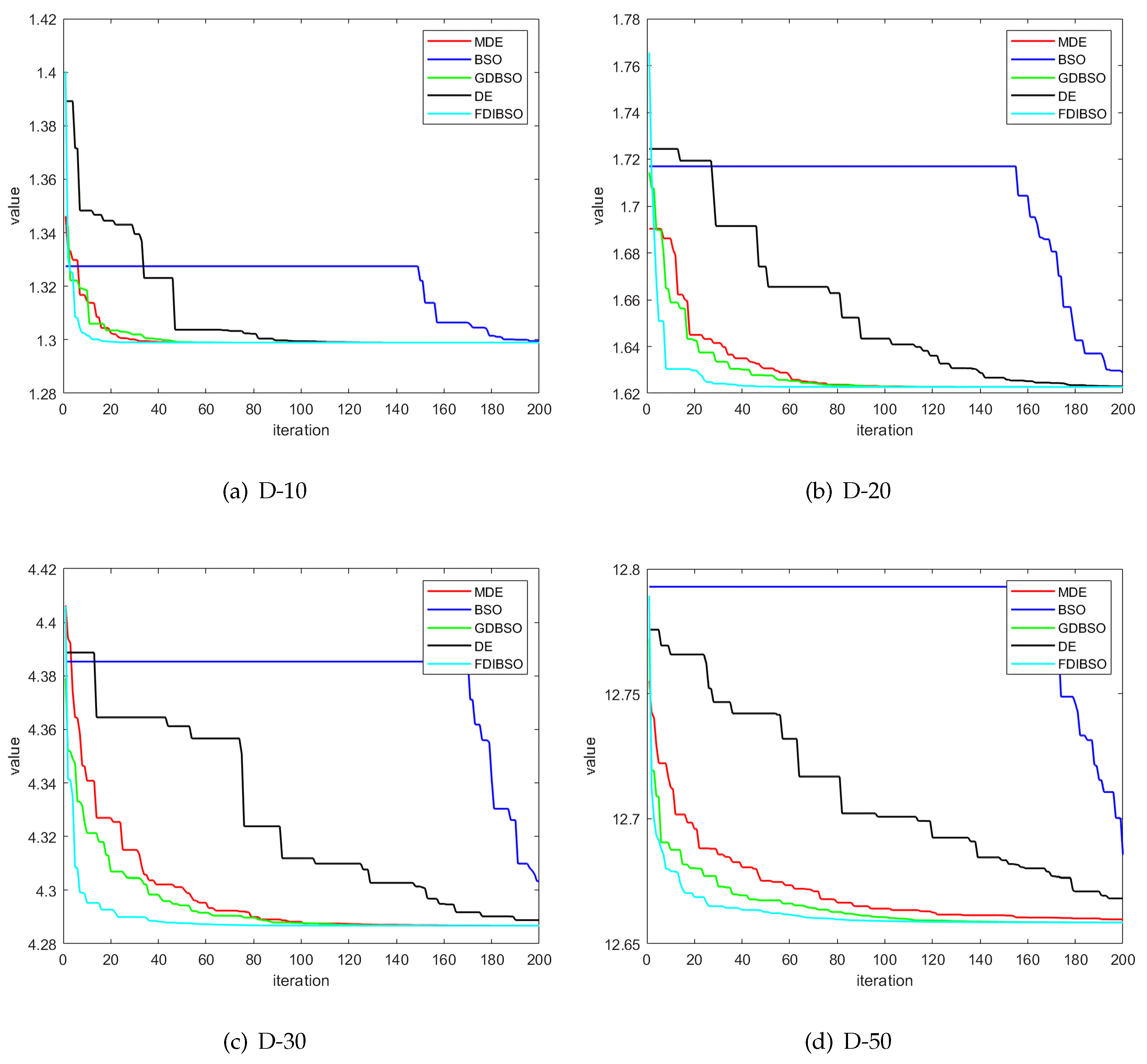
In response to the issues mentioned above, this paper introduces the FDIBSO algorithm, which has higher optimization performance, into the model’s solution process to achieve a more accurate assessment of AUV intelligence. In order to examine the performance gap between the FDIBSO algorithm and the comparative algorithms at higher dimensions, this paper employs the Monte Carlo method to generate multiple sets of simulated weights. The experiments limited the number of iterations to 200. The speed at which each algorithm converged was assessed across three conditions with 10, 20, 30, and 50 dimensions, with the results depicted in Figure 5. Additionally, to ensure consistency in experimental testing of the comparative algorithms, the performance of other BSO variants used in the CEC2018 experiments, including ADMBSO and DDGBSO algorithms (the GDBSO algorithm has already been compared), was tested. The results are shown in Figure 6. The mean convergence time required to achieve the optimal solution was calculated and documented in

Table 7. The mean convergence time of each algorithm (unit: seconds).

Algorithm	BSO	DE	MDE	GDBSO	FDIBSO
Mean (D-10)	1.65	0.24	0.13	0.22	0.33
Mean (D-20)	No	0.55	0.26	0.47	0.51
Mean (D-30)	No	No	0.53	0.82	0.98
Mean (D-50)	No	No	No	1.44	1.72

and

Table 8. The mean convergence time of different BSO variants (unit: seconds).

Algorithm	BSO	ADMBSO	DDGBSO	GDBSO	FDIBSO
Mean (D-10)	1.65	0.27	0.13	0.22	0.33
Mean (D-20)	No	0.67	0.53	0.47	0.51
Mean (D-30)	No	1.03	0.77	0.82	0.98
Mean (D-50)	No	2.23	1.49	1.44	1.72

. A “No” in the table means the algorithm cannot find a global optimal solution within the given number of iterations.

First, whether comparing various BSO variant algorithms or comparing the several algorithms used in reference [36], the FDIBSO algorithm proposed in this paper demonstrates the best convergence performance when solving the MMCW model. In addition, the advantage of the FDIBSO algorithm is more evident with the increase in dimensions under the four conditions. Second, under the limit of 200 iterations, some algorithms cannot find the global optimal solution under some dimensional conditions. However, the FDIBSO algorithms can all find the global optimal solution with the minimum number of iterations. When comparing the mean convergence time, the FDIBSO algorithm, due to the use of spectral clustering, leads to an increased time complexity. Although it is not advantageous compared to some other BSO algorithm variants, it is only inferior to the DDGBSO and GDBSO algorithms and is better than the ADMBSO algorithm.

The experimental findings indicate that, in terms of computing weights for AUV intelligence evaluation, the FDIBSO algorithm exhibits superior overall performance.

5. Discussion

Drawing upon the experimental outcomes detailed in Section 4.2 and Section 4.3, it is evident that the FDIBSO algorithm possesses several advantages. First, the FDIBSO algorithm demonstrates superior optimization precision compared to other variations of the BSO algorithm, showcasing its ideal advantage. The FDIBSO algorithm can achieve optimal optimization search results on more than half of the functions featured in the CEC2018. This assertion is supported by the data in Table 1, Table 2, Table 5 and Table 6. Second, the optimization precision of the FDIBSO algorithm holds a distinct edge over other contemporary competitive intelligent algorithms. The results show that although the FDIBSO algorithm achieve the same level of effectiveness as the MFO-SFR algorithm, it performs better at some functions and significantly outperforms other intelligent algorithms. This assertion is substantiated by Table 3 and Table 4. Third, the rate of convergence for the FDIBSO algorithm does not match the velocity of some BSO variants in the early stage, but with advancement of iterations, the convergence speed can be realized to overtake that of the other algorithms. This assertion is supported by Figure 3 and Figure 4. Fourth, although the FDIBSO algorithm is slightly inferior in time complexity to some BSO variant algorithms when calculating the MMCW model, its convergence performance is superior to all algorithms. It can converge to the optimal solution with the fewest iterations for problems with various dimensions, thus improving the accuracy of weight calculations. The conclusion can be confirmed by Figure 5 and Figure 6 and Table 7 and Table 8.

Numerous experiments have confirmed FDIBSO’s advanced efficacy over prior enhanced BSO algorithms. As an innovative approach influenced by human behavioral patterns, FDIBSO has shown significant promise for tackling intricate optimization issues. Additionally, incorporating the flock decision mutation strategy, good point set, and spectral clustering method within FDIBSO encourages the development of more innovative approaches for increasingly complex challenges. Moving forward, FDIBSO is set to tackle high-dimensional and large-scale applications.

Future studies may explore several avenues: further improving the optimization accuracy of the FDIBSO algorithm on all tested functions, improving the algorithm’s convergence speed in the early stage, and utilizing the BSO algorithm for more real-world engineering optimization challenges.

6. Conclusions

This study introduces the improved brain storm optimization algorithm based on the flock decision mutation strategy. First, the flock decision mutation strategy is proposed to improve the BSO algorithm’s optimization accuracy for various optimization issues. Second, the good point set and spectral clustering are integrated within the BSO algorithm, enhancing the algorithm’s population diversity and clustering accuracy. Third, this paper compares and analyzes FDIBSO and the BSO, ADMBSO, GDBSO, DDGBSO, MSWOA, HOA, WMFO, and MFO-SFR algorithms. The results show that for the MMCW model in AUV intelligence evaluation and many benchmark functions from the CEC2018, the FDIBSO algorithm has the best performance.