Abstract
Control charts are tools of paramount importance in statistical process control. They are broadly applied in monitoring processes and improving quality, as they allow the detection of special causes of variation with a significant level of accuracy. Furthermore, there are several strategies able to be employed in different contexts, all of which offer their own advantages. Therefore, this study focuses on monitoring the variability in univariate processes through variance using the Binomial version of the ATTRIVAR Same Sample S2 (B-ATTRIVAR SS S2) control chart, given that it allows coupling attribute and variable inspections (ATTRIVAR means attribute + variable), i.e., taking advantage of the cost-effectiveness of the former and the wealth of information and greater performance of the latter. Its Binomial version was used for such a purpose, since inspections are made using two attributes, and the Same Sample was used due to being submitted to both the attribute and variable stages of inspection. A computational application was developed in the R language using the Shiny package so as to create an interface to facilitate its application and use in the quality control of the production processes. Its application enables users to input process parameters and generate the B-ATTRIVAR SS control chart for monitoring the process variability with variance. By comparing the data obtained from its application with a simpler code, its performance was validated, given that its results exhibited striking similarity.
1. Introduction
Control charts were initially introduced by [1] and are the primary and most technically sophisticated tools of statistical process control [2]. They are widely employed in process monitoring and serve to detect nonconformities and special causes of variation, thus enabling the early identification of disturbances aimed to minimize negative adverse financial impacts [3].
Among control charts, some utilize variable inspection for monitoring continuous quality characteristics, while others employ attribute inspection, which was initially designed for monitoring non-continuous quality characteristics.
One of which is grounded on the numerical measurements of quality characteristics, and another is based on the attributes defined by [4] as quality characteristics measured in a nominal scale or categorized according to a predetermined scheme of labels. For instance, classifying fruits as being good or rotten, and nails or screws as defective or not defective.
Although the primary purpose of attribute inspection was outlined about 70 years ago, researchers have made contributions by suggesting their use for controlling continuous quality characteristics, and more recent studies have proposed better means for such [5].
There are numerous comparisons between variable and attribute charts in the literature, such as [5,6,7,8,9,10]. These authors emphasize the superior efficiency and informativeness of variable inspection due to its reliance on measurements, as opposed to a simpler, faster, and cheaper application of attribute inspection.
Several researchers explore the use of attribute inspections for continuous characteristics, such as [8,9,11], in an attempt to continuously seek to improve the efficiency of resource utilization and improve the performance of control charts.
Ergo, what once meant having to use a sample 6.667 times larger in attribute charts to achieve the same level of performance as variable charts [2] now requires a sample less than twice as large using the proposed by [9].
The strategy of using variable and attribute inspections combined into a single chart had initially been proposed by [12] and is similar to one which was later on called as ATTRIVAR (ATTRIbute + VARiable) by [5]. Thenceforth, these mixed charts combine the advantages of both forms of inspection initially called as such.
A version of [12] consisted in designing the (attribute) and (variable) charts separately and dividing the collected sample into two subsamples. Then, the former was submitted to chart evaluation, and the latter was submitted to chart evaluation if the former had been rejected.
Ref. [7] also proposed a mixed chart without subdividing the sample and used the same sample in both stages of inspection (as in [13,14], and to the proposal herein). Ref. [5] proposed ATTRIVAR-1 chart, which uses the same sample in both stages, in addition to ATTRIVAR-2 chart, which makes use of different samples. In this work, the terminologies SS (same sample) and DS (different sample) refer to these strategies, respectively.
Unlike these proposals, which addressed only mean monitoring, Ref. [10] proposed a mixed chart to monitor variability through variance. The authors coupled the chart from [9] in the stage of attribute inspection with the S2 chart in the stage of variable inspection using different samples.
Afterwards, Ref. [15] proposed the Trinomial version of the ATTRIVAR (T-ATTRIVAR) chart aimed at mean monitoring but using three attributes in the first inspection stage instead of two as in other strategies.
Thus, this paper explores the Binomial version of ATTRIVAR Same Sample S2 (B-ATTRIVAR SS S2) chart that makes use of the first inspection stage with two attributes (“binomial”) using the same sample in both inspection stages (“same sample”) to monitor the process variance (S2).
Although there is a certain number of works on control charts coupling attribute and variable inspections in the literature, research on monitoring the variability of univariate processes through variance, i.e., B-ATTRIVAR SS S2, is still lacking. The novelty of this study lies in proposing an interface capable of receiving input data from a user thereof, to obtain control limits through simulations and generate a (B-ATTRIVAR SS S2) chart so as to monitor the variability of a univariate process.
The control chart strategy proposed herein is similar, particularly to those from: Ref. [9], as both make use of attribute inspections to monitor the process variance, Ref. [10], given that the attribute and variable data were also used to monitor process variance, and [15], who proposed the most similar strategy but used it to monitor process mean using three attributes in the first monitoring stage (instead of two as in this study).
Even though in-control process parameters are usually unknown in practice and require estimates using historical data, this paper focuses on monitoring processes where these parameters are known [16].
In addition to advances in statistical process control strategies, an integration of computer interfaces is also crucial to increase the manufacturing system’s efficiency. As discussed by [17], the convergence between digital models and physical industrial environments using data is of paramount relevance to smart manufacturing. This is due to the fact that it can provide interaction and information exchange between software, the computational interfaces, and the physical systems of manufacturing processes.
In this context, the application of computational interfaces offers new possibilities for monitoring and controlling industrial processes in real time. Although this work mainly focuses on introducing an interface developed using R and Shiny to monitor process variability, it is also worth mentioning the potential of integrating it with industrial digital systems, such as manufacturing execution systems (MES). Despite not being directly discussed in this study, the role of MES in facilitating quality monitoring and process optimization is also worth being mentioned. The authors of [18] explain that MES can provide a useful platform in quality monitoring, as it allows direct data acquisition and the monitoring of quality parameters’ variability. Ref. [19], for instance, explores the possibilities of using control charts to analyze the data stored in MES and provide feedback to the systems aiming to optimize production parameters.
This manuscript is organized as follows: Section 2 describes the B-ATTRIVAR SS S2 chart and draws a comparison with more usual charts; Section 3 explains how its application was conceived and the manner in which the results have been achieved; Section 4 presents its interface and operation, as well as a validation of its results; and Section 5 draws its conclusion and proposes suggestions for future works.
2. Chart B-ATTRIVAR SS S2
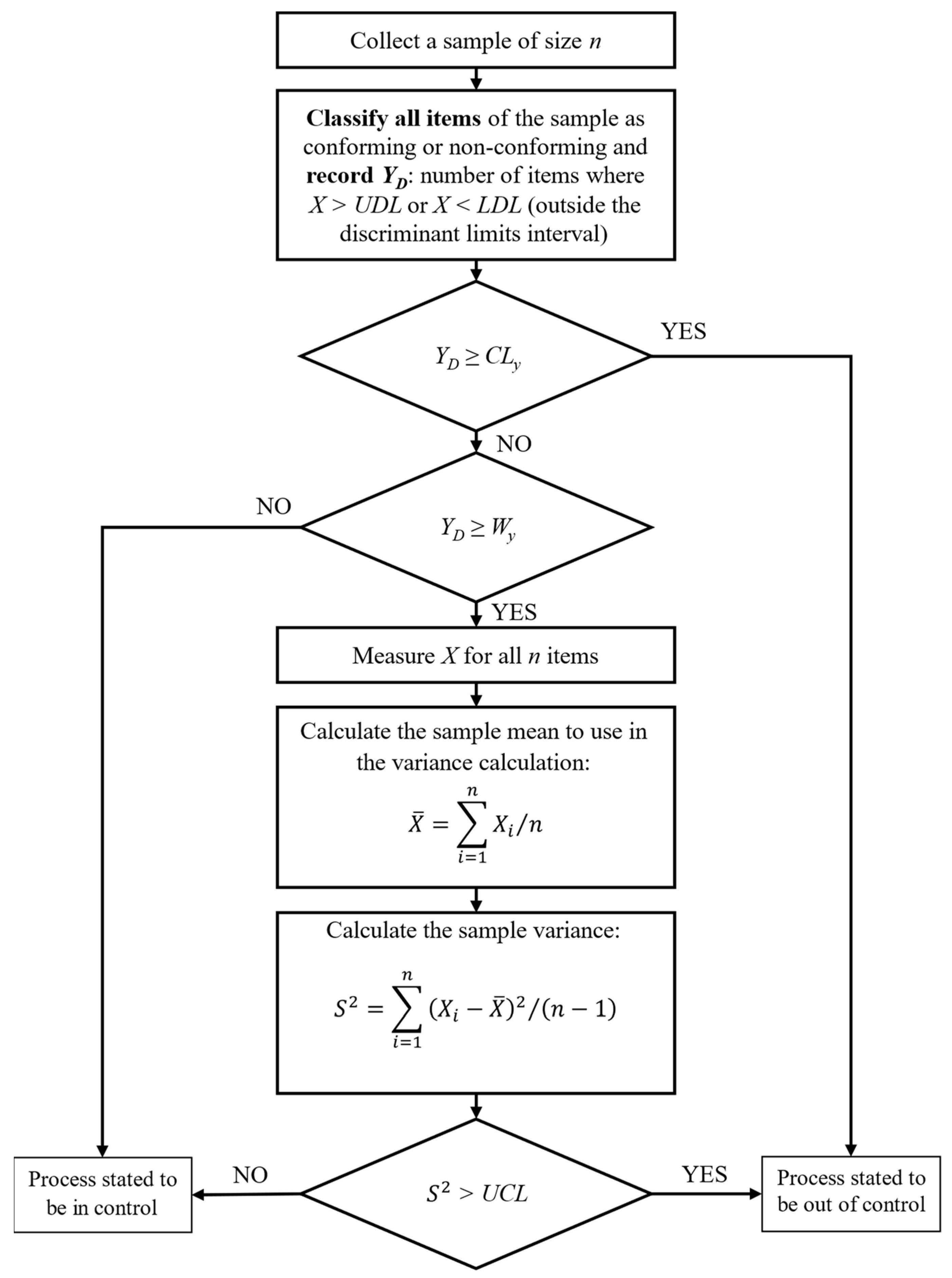
After sample collection, all n items of the B-ATTRIVAR SS S2 chart are inspected based on attribute, similarly to the from [9]. These inspections make use of some device (such as a go/no-go gauge, for example) configured using the discriminant control limits (lower discriminant limit) and (upper discriminant limit). Each item outside these limits is classified as nonconforming. After classifying all items in the sample, is recorded as the number of rejected items. If ≥ (attribute control limit), the process is defined as being out of control. Conversely, it is assessed whether < (warning attribute control limit). If so, it is found that the process is in control. If otherwise, the variable inspection process is initiated using the same sample.
The stage of variable inspection is performed similarly to that in the classic S2 chart described by [2,4], in which quality is measured based on all n items in the sample, and variance S2 is calculated. If S2 is outside the acceptance interval defined by (variable lower control limit) and (variable upper control limit), the process is defined as being in control. Otherwise, it is out of control. This entire process is depicted in Figure 1.

Figure 1.
Flowchart of the B-ATTRIVAR SS S2 Chart.
It is worth mentioning that it is common to use only the upper control limit to inspect variable S2, as a process should have the least possible variability, as mentioned by [20], given that this strategy makes the chart more effective at detecting increases in process variance. In such a case, is denoted as .
In this paper, both the attribute and variable inspection limits are optimized to achieve acceptable performance values determined by and , or by α and β, considering that refers to the average run length or the average number of samples collected until the chart signals for the first time, in addition to the fact that [4]:
where α is the probability of type I error, β is the probability of type II error, the index “0” indicates a process in control, and index “1” indicates a process being out of control.
The performance of the B-ATTRIVAR SS S2 chart (mixed inspection) was compared to that of S2 (variable inspection) and np (attribute inspection) charts, as in Table 1, which shows simulated values with sample sizes of 5 (n = 5) by varying the standard deviation of simulated samples through λ in each row. The results demonstrate a similar performance of the studied chart to that of the np chart. Nevertheless, it is still worth mentioning its advantages over the np charts, mainly on account of the fact that the quality characteristic measurements required in the stage of variable inspection of the B-ATTRIVAR SS S2 are capable of providing valuable information to enhance the process analysis and make improvements. Although the performance of the ATTRIVAR proved inferior to that of the S2 chart, it still offers notable advantage over it, i.e., its operational simplicity [14].

Table 1.
Comparison of the performance of charts for monitoring S2 with n = 5.
3. Application Development
The application was developed using the RStudio development environment, which is free and offers various packages and functionalities available for installation using a computational programming based on the R language. According to [21], R is ranked among the 10 most popular programming languages used globally and has become a fundamental computational tool for research in various areas, such as statistics, mathematics, physics, chemistry, medicine, among others.
Additionally, the Shiny package was used for interface development, which, according to [21], was launched in 2012 and has continuously gained popularity in developing interactive websites using R language functionalities.
The average run length () was used for measuring the efficiency or performance of control charts. Ref. [22] considers it as the best-known and most widely used method to measure and analyze control chart performance.
3.1. Inputs and Outputs Definition
Regarding the development of a B-ATTRIVAR SS control chart application aimed to monitor the variability of univariate processes through variance, the code should be capable of generating control limits for the attribute ( and ) and variable ( and , or just if ) inspections. Based on these four outputs, the application can effectively perform the primary function of a control chart: either accepting or rejecting samples to classify the process as being in control or out of control.
For such a purpose, the initial necessary inputs would be sample size (n), mean (), and standard deviation () of the process, given that they are essential parameters for the program to perform normal sample simulations.
The user would have to provide the maximum desired probability of a type I error () and the maximum desired probability of a type II error () for a given variation (λ) in standard deviation to obtain the attribute and variable control limits. Thus, would define the min and for a given λ, which would define the max . Then, it would be possible to determine the acceptance intervals, as and are directly related to the control limits.
To start the first stage of monitoring with attribute inspection, The user would have to determine the discriminant limits and , which were also defined as outputs. Thus, these values could be configured using a go/no-go gauge device, for instance. Afterwards, they could conduct inspections and input the number of nonconforming items in each sample into the application to proceed to the next stage.
Furthermore, the user would have to provide the maximum percentage of samples to be submitted to variable inspection (%) to define the discriminant limits ( and ).
3.2. Obtaining Control Limits
The process of obtaining control limits was expected to be performed through simulations and trial-and-error iterations. Its logical is that the program makes the first iteration using lower values for the control limits, and it comes to %S2, α or β in each iteration. Then, the program verifies whether these values are lower than the maximum values established by the user, and it changes the limits and proceeds to the next iteration if otherwise.
To enhance code organization, it was segmented into four sections, namely, A, B, C1, and C2. Each having a beginning and an end, and their own iterations able to calculate and record the results in the form of a matrix.
In section A, it explores the possible combinations of and to derive the smallest discriminant limits ( and ) satisfying the % condition:
where NV is the number of samples, which would be submitted to variable inspection, and TN is the total number of simulated samples.
For such a purpose, it simulates one million samples from a normal distribution based on user-defined parameters (n, μ, and σ) for in-control conditions, and calculates how many would undergo variable inspection, i.e., . Then, it performs the test described in Equation (4). This entire process repeats until the condition is satisfied.
In section B, it accesses each combination of and , but using the values of and for each, and proceeds to obtain the smallest variable control limits ( and ) meeting the requirement of :
For such, it simulates samples under control and submits them to attribute inspections and to variable inspections whenever necessary, until it reaches ten thousand signals. Then, it records the number of simulated samples until each signal’s emission, thus allowing it to calculate by computing the arithmetic mean of these ten thousand recorded numbers. Afterwards, it assesses the condition of Equation (5) and repeats this until it is satisfied by incrementing the upper limit and decrementing the lower limit during each iteration, as shown in the Equations (6) and (7). For each combination of , , , and , it assigns the following values to limits by ever incrementing the absolute value of parameter L:
Within section C1, it already has recorded the various combinations of , , , , , and , and it assesses whether each of them meets the requirement set by the user:
For such, it simulates normal samples, albeit out of control, by altering only the standard deviation to (where λ and σ are defined by the user). These samples undergo the entire B-ATTRIVAR SS S2 chart flow using the parameters from each obtained combination. Consequently, is calculated for each combination (similarly to ) and it is tested whether Equation (8) is satisfied. This process is carried out only once for each parameter combination, and it records which combinations can meet this requirement.
In section C2, it accesses combinations meeting the requirement and selects the best solution as the one with the lowest calculated .
Definite results can be seen by the user and are used by the program to perform other steps and ensure the functioning of the control chart itself. The displayed parameters are: n, , , , , , , %S2, , , α, λ, and .
4. Results
Given the objective of developing an interface to enable the utilization of the B-ATTRIVAR SS S2 chart, it is necessary to initially understand the expected usage dynamics through which the application was conceived.
At first, the application user is expected to input the initial parameters required for obtaining the control limits (as described earlier). Once the program finishes obtaining them, the user should be able to visualize a chart showing horizontal lines representing the control limits and should input the of their sample, which can be plotted on the chart. If is between and , something users can verify on the chart, they should input the quality characteristic measurements for all items in the sample. Therefore, the program should calculate and plot sample variance on the chart, and the signal if it somewhat indicates that the process is out of control.
4.1. The Interface
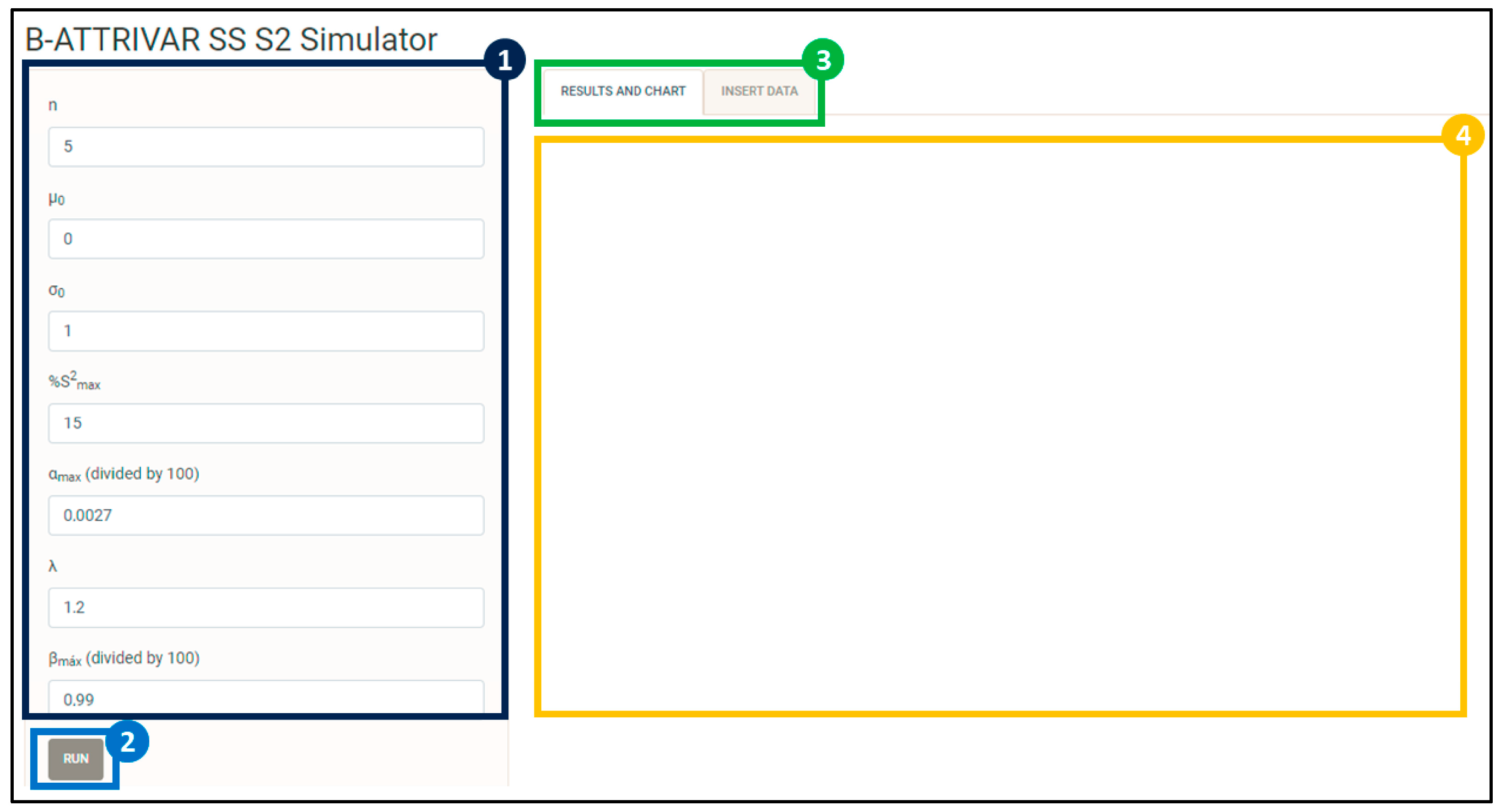
The main layout of its interface was configured as depicted in Figure 2. In the area marked with the number one, there is a sidebar with fields where the user can input values or keep the predefined values in the program (shown in Figure 2). Below this sidebar, in the area marked with the number two, there is the RUN button which the user should click on to execute the code and obtain the results. Adjacent to this, in the area marked with the number three, there are the two tabs of the application, between which the user can switch by clicking on one of them. At the bottom, the area marked with the number four represents where the results of calculations and the chart itself are displayed in the RESULTS AND CHART tab; and the editable table to insert sample data in the INSERT DATA tab.
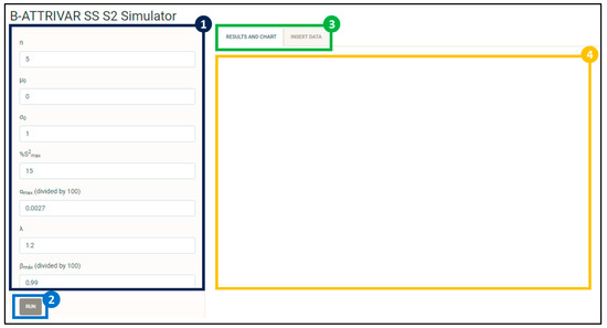
Figure 2.
Main layout of the developed interface.
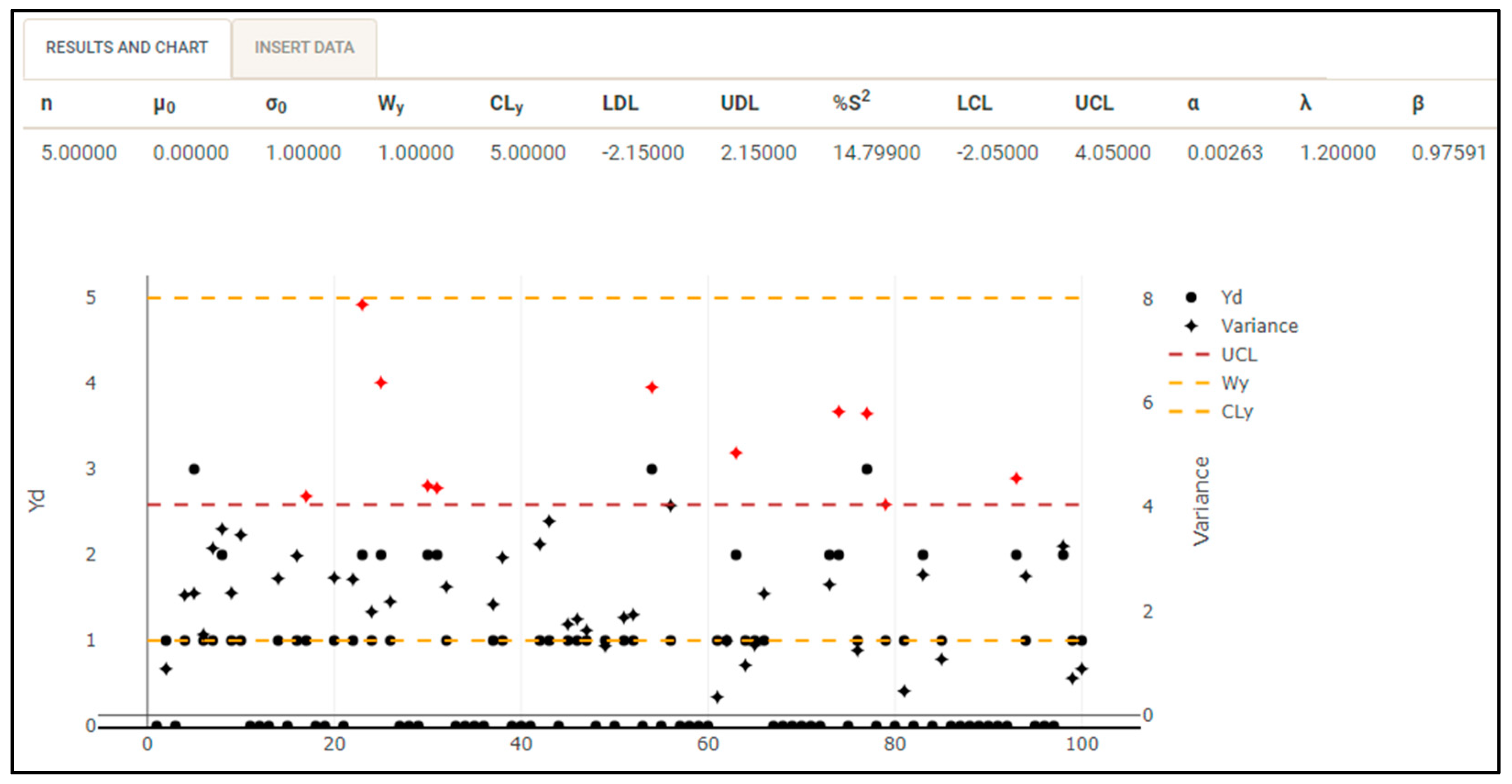
After pressing the RUN button, the end results and the chart are displayed in the RESULTS AND CHART tab, as shown in Figure 3.
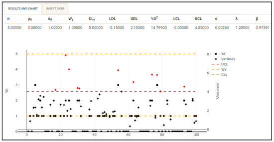
Figure 3.
Results and chart displayed in the interface.
Some parameters entered by the user (n, , e λ) are shown below the tab names and above the graph, along with the results found for other parameters through simulations and calculations (, , , , %S2, , , α, ).
4.2. The Chart
Bearing a resemblance to the charts presented by [13,14,15], Figure 3 shows an x-axis representing the sample number, and two y-axes: one for on the left side and another for sample variance on the right side.
The chart displays the limits of and on the axis, and on the variance axis, all represented as dashed lines. The circular points represent the data series, while the differently shaped points represent the calculated sample variance data series. It is crucial to highlight that the points representing sample variance will be plotted only if , due to the fact that samples satisfying < are accepted and those within ≥ are rejected in the B-ATTRIVAR SS chart, and thus do not need to be submitted to variable inspection in both cases.
Points are standardly plotted in black. However, they are shown in red to represent signals (when samples are rejected for instance) to display if they occur in the attribute inspection (circular points) or variable inspection (non-circular points).
The chart is rather dynamic, as any changes in the editable table data lead to automatic adjustments in the plotted points on the chart. Additionally, users can press and hold the mouse button on either of the two abscissa axes to drag them upwards or downwards, thus moving both their labels and associated points. Furthermore, users can zoom in and out by pressing and holding the mouse button over any point in the plot area, then dragging it to form a rectangle defining the area to be zoomed.
4.3. The Editable Table
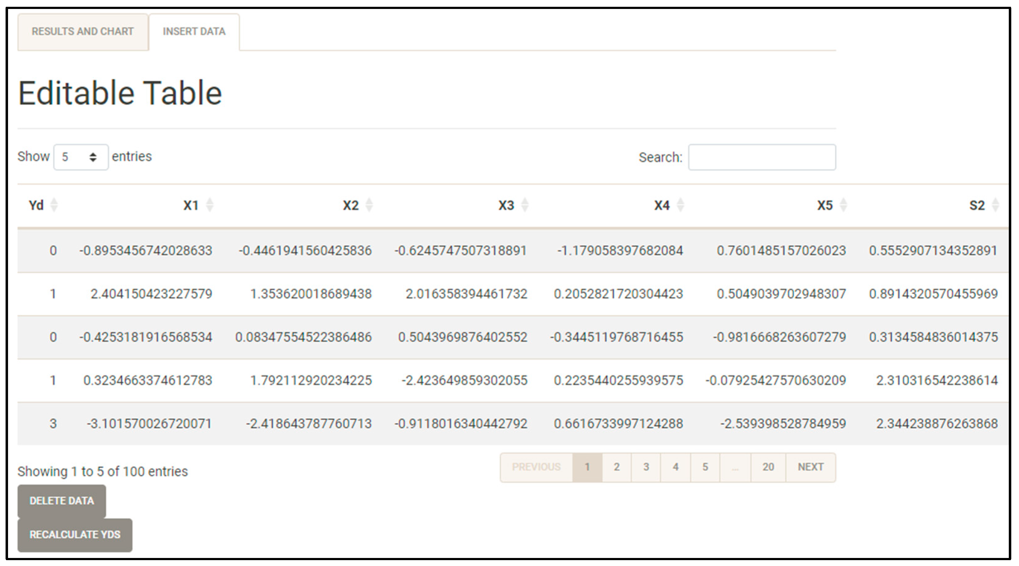
The data plotted on the chart are from the editable table illustrated in Figure 4 and located in the INSERT DATA tab. It contains some columns dependent on the user-inputted n value, although the first and last columns always represent and the calculated variance of each sample, respectively, regardless of the inputted n value. Other columns between the first and the last ones are intended for inputting quality characteristic measurements, and thus depend on the sample size (n = 5 in the case of Figure 4, and therefore there are 5 columns for measurements).
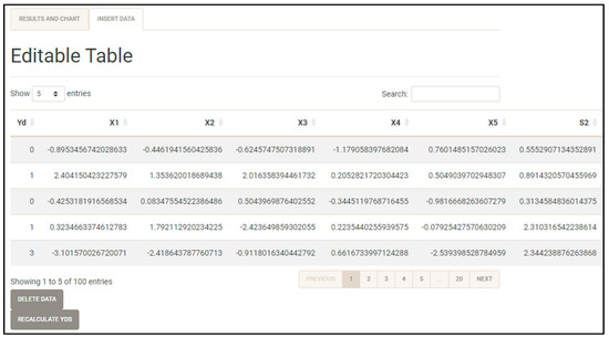
Figure 4.
Editable table on the interface.
All the columns are editable, except for the last one. Although the user can attempt to change its value, the table automatically recalculates it, since the variance values cannot be arbitrary, but are rather calculated from the quality characteristic measurements.
Before users start monitoring any process, the application offers a preview of its functionality. It generates data for 100 out-of-control samples from a normal distribution, then it submits them to inspections with the definite results of the control limits and plots them on the chart. After clicking on the RUN button at the sidebar, once the results are obtained, the application automatically displays data about the 100 samples in both the table and the chart.
The editable table standardly displays only five rows, but just below the Editable Table title, the number of rows can be changed by clicking on Show 5 entries and altering them to the desired number.
Below the table, there are the DELETE DATA and RECALCULATE s buttons. All the values recorded in the table are deleted by pressing the first button, leaving all fields empty for new data input and, consequently, erasing all the plotted points on the chart. The second button recalculates all s in the table’s first column based on the values of the monitored quality measurements.
Naturally, as previously explained, according to the logic of monitoring a process through an ATTRIVAR chart, the user can start inspections via attribute without conducting any measurements, which is one of the main advantages of this strategy compared to variable control to avoid excessive measurements. These can often be expensive and/or excessively time-consuming; thus, it would be irrelevant to calculate through measurements.
Moreover, it would also be unreasonable if the user altered any measurement data and if remained the same, even though the number of nonconforming items might have changed. Furthermore, automatically calculating this column would be inappropriate as well, since it would not allow the user to input regardless of the measurements, which would contradict the inherent logic of the ATTRIVAR strategy.
Therefore, the fields are editable so that the user can input the number of nonconforming items for each sample. Additionally, a button is provided for the user to click upon at any time to recalculate all in the table based on the measurements.
4.4. Results Validation
Theoretical calculations of the parameters of this chart have not been identified. Therefore, a simpler code was developed to simulate the ARLs of the B-ATTRIVAR SS S2 chart aiming to validate the application’s results and ensure the consistency of simulations and control limit calculations. Control limits are set in it, and it calculates ARLs for different values of λ.
Hence, to validate the application results, the control limits generated by the application were utilized as input parameters for the code. Subsequently, the results obtained from both methods were compared in terms of %S2, , and . The reasons for selecting these parameters are as follows:
- Analyzing whether %S2 verifies if the chart submits the expected percentage of samples in the stage of variable inspection;
- Analyzing whether verifies if the chart commits to the type I error after the expected number of tested samples is calculated;
- And analyzing whether verifies if the chart detects a signal at the expected speed, or after the expected number of tested samples is calculated.
As shown in Table 2, several scenarios were tested, all being and , and the columns labeled as “reference” correspond to the values obtained through the simpler code.

Table 2.
Results comparison and validation (μ0 = 0, σ0 = 1).
The first five rows on the table represent the execution of simulations with default values set on the application interface, as in Figure 2. In the next five rows, the application was executed only by changing the % parameter from 15% to 10%. The next nine rows contained changes not only in % but also in n and λ. This approach enables the analysis of whether alterations in one or more parameters affect the validity of its results.
Its results demonstrate a strong consistency with those obtained through the reference code, i.e., %S2, , and show notably similar values. For instance, the largest percentage differences observed in the Δ and Δ columns were 5.66% and 2.77%, respectively.
4.5. Example
To exemplify how the proposed application functions, the code was run using the default values for inputs (the same values set in the interface fields shown in Figure 3). After having calculated control limits as described in Section 3.2, the application is ready to be used for process monitoring.
In this example, the simulations converged to the following values for control limits: ; ; and .
Although the application was designed with the purpose of allowing the user to start monitoring via the attribute inspections, the following example is a simulation. Therefore, as shown in Table 3, 25 random (out of control) samples of measurements were generated and were calculated from them. For samples where is between and limits, the variances were calculated (S2).

Table 3.
Example data.
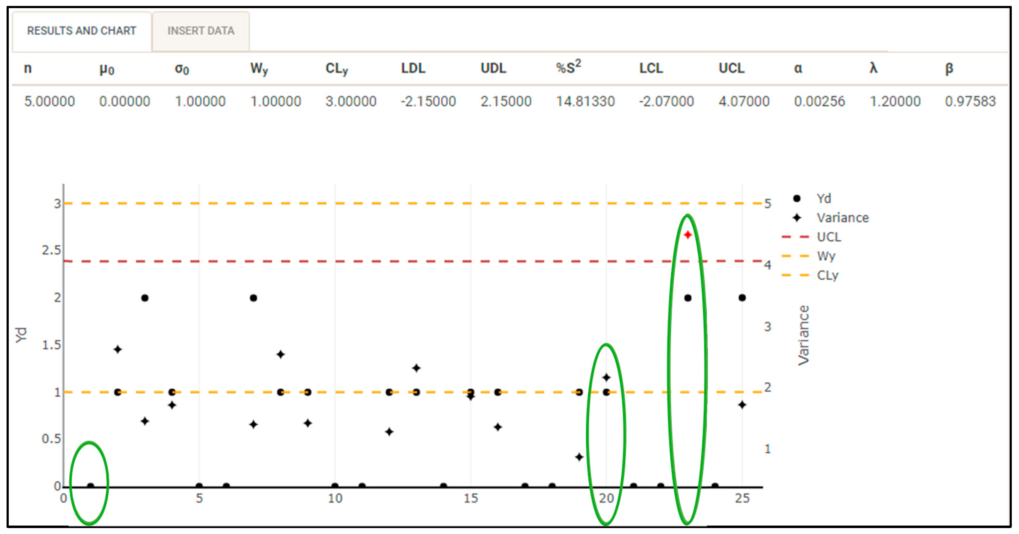
Figure 5 shows how the interface plots data from Table 3. As aforementioned, the of all samples are plotted as circular points, and S2 are plotted as non-circular points whenever necessary.
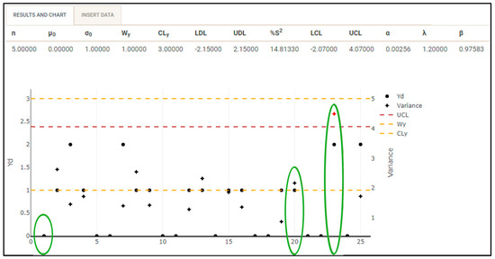
Figure 5.
Example chart.
The first sample highlighted in the chart is a case where and S2 does not need to be calculated thereof (as shown in Table 3), thus not being plotted in the chart (as in Figure 5).
The twentieth sample, also highlighted in the chart, is a case where . Thereby, S2 is calculated and plotted, since , and the variance is plotted in black in this example.
Similarly, the twenty-third sample, also circled in the chart, is a case where is also within the range of attribute control limits, and the variance is calculated and plotted. However, and the chart signals plotting the variance are in red.
Likewise, in cases where , the chart signals that the process is out of control, and is plotted in red.
5. Conclusions
In this study, an interface was developed to generate and display control limits for the B-ATTRIVAR SS S2 chart, enabling the real-time monitoring of process variance. It was achieved through inputting process data and user-defined requirements, and the program uses these data to compute the control limits and render a chart showing them and sample data. Once users have their process data, they can input it and use the control chart to monitor process variability. Although the application has not been tested in actual processes, its results have been validated in this study through comparisons with reference values, thus revealing low percentage deviations.
As an opportunity for improvement and further research, it is imperative to explore methods to reduce its execution time. Due to multiple iterations aimed at generating more precise results, the program might last a significantly long execution time depending on the device on which it is run. One potential approach to face this challenge is leveraging artificial intelligence tailored for optimizing code performance.
Furthermore, investigating the feasibility of adapting the application to integrate it with business and industrial systems, such as manufacturing execution systems (MES), could enhance its versatility and potential for automation across various industrial applications, including real-time production monitoring and control.
Moreover, future research should analyze the influence of variations in input parameters on results, in addition to conducting extensive studies and interface development aimed to consider the application of the proposed control strategy using estimated parameters, thereby extending its applicability. Furthermore, exploring methods for theoretically and mathematically deriving the ARLs and control limits of the proposed strategy would be of significant interest.
Author Contributions
Conceptualization, J.P.C.V. and M.A.G.M.; methodology, A.d.S.M. and T.S.A.; software, J.P.C.V. and A.d.S.M.; validation, M.A.G.M. and T.S.A.; formal analysis, J.P.C.V., M.A.G.M., A.d.S.M. and T.S.A.; investigation, J.P.C.V. and M.A.G.M.; resources, A.d.S.M. and T.S.A.; data curation, J.P.C.V., M.A.G.M., A.d.S.M. and T.S.A.; writing—original draft preparation, J.P.C.V., M.A.G.M., A.d.S.M. and T.S.A.; writing—review and editing, J.P.C.V., M.A.G.M., A.d.S.M. and T.S.A.; visualization, J.P.C.V., M.A.G.M., A.d.S.M. and T.S.A.; supervision, M.A.G.M.; project administration, M.A.G.M.; funding acquisition, M.A.G.M. All authors have read and agreed to the published version of the manuscript.
Funding
This research received no external funding, and the APC was founded by São Paulo State University under process EDITAL PROPG 16/2024.
Data Availability Statement
No new data were created or analyzed in this study. Data sharing is not applicable to this article.
Acknowledgments
Thanks to PIBIC/CNPq-EDITAL 2020 and CNPq process 307945/2019-7.
Conflicts of Interest
The authors declare no conflicts of interest.
References
- Shewhart, W.A. Economic Control of Quality of Manufactured Product, 1st ed.; D. Van Nostrand Company: Nova York, NY, USA, 1931. [Google Scholar]
- Montgomery, D.C. Introduction to Statistical Quality Control, 6th ed.; John Wiley & Sons: Hoboken, NJ, USA, 2009. [Google Scholar]
- Ali, S.; Abbas, Z.; Nazir, H.Z.; Riaz, M.; Zhang, X.; Li, Y. On developing sensitive nonparametric mixed control charts with application to manufacturing industry. Qual. Reliab. Eng. Int. 2021, 37, 2699–2723. [Google Scholar] [CrossRef]
- Aslam, M.; Saghir, A.; Ahmad, L. Introduction to Statistical Process Control, 1st ed.; John Wiley & Sons: Hoboken, NJ, USA, 2020. [Google Scholar]
- Ho, L.L.; Aparisi, F. Attrivar: Optimized control charts to monitor process mean with lower operational cost. Int. J. Prod. Econ. 2016, 182, 472–483. [Google Scholar] [CrossRef]
- Aparisi, F.; Ho, L.L. M-ATTRIVAR: An attribute-variable chart to monitor multivariate process means. Qual. Reliab. Eng. Int. 2018, 34, 214–228. [Google Scholar] [CrossRef]
- Aslam, M.; Azam, M.; Khan, N.; Jun, C.H. A mixed control chart to monitor the process. Int. J. Prod. Res. 2015, 53, 4684–4693. [Google Scholar] [CrossRef]
- Bezerra, E.L.; Ho, L.L.; Quinino, R.d.C. GS2: An optimized attribute control chart to monitor process variability. Int. J. Prod. Econ. 2018, 195, 287–295. [Google Scholar] [CrossRef]
- Ho, L.L.; Quinino, R.C. An attribute control chart for monitoring the variability of a process. Int. J. Prod. Econ. 2013, 145, 263–267. [Google Scholar]
- Ho, L.L.; Quinino, R.d.C. Combining attribute and variable data to monitor process variability: MIX S 2 control chart. Int. J. Adv. Manuf. Technol. 2016, 87, 3389–3396. [Google Scholar] [CrossRef]
- Wu, Z.; Khoo, M.B.C.; Shu, L.; Jiang, W. An np control chart for monitoring the mean of a variable based on an attribute inspection. Int. J. Prod. Econ. 2009, 121, 141–147. [Google Scholar] [CrossRef]
- Sampaio, E.S.; Ho, L.L.; de Medeiros, P.G. A combined control chart to monitor the process mean in a two-stage sampling. Qual. Reliab. Eng. Int. 2014, 30, 1003–1013. [Google Scholar] [CrossRef]
- Leoni, R.C.; Costa, A.F.B. The performance of the truncated mixed control chart. Commun. Stat.-Theory Methods 2019, 48, 4294–4301. [Google Scholar] [CrossRef]
- Costa, A.F.B.; Neto, A.F. Monitoring the process mean with an ATTRIVAR chart. Commun. Stat.-Theory Methods 2022, 51, 4903–4920. [Google Scholar] [CrossRef]
- Simões, F.D.; Costa, A.F.B.; Machado, M.A.G. The Trinomial ATTRIVAR control chart. Int. J. Prod. Econ. 2020, 224, 1–8. [Google Scholar] [CrossRef]
- Faraz, A.; Heuchenne, C.; Saniga, E. An exact method for designing Shewhart and S2 control charts to guarantee in-control performance. Int. J. Prod. Res. 2018, 56, 2570–2584. [Google Scholar] [CrossRef]
- Xia, K.; Sacco, C.; Kirkpatrick, M.; Saidy, C.; Nguyen, L.; Kircaliali, A.; Harik, R. A digital twin to train deep reinforcement learning agent for smart manufacturing plants: Environment, interfaces and intelligence. J. Manuf. Syst. 2021, 58, 210–230. [Google Scholar] [CrossRef]
- Gendre, Y.; Waridel, G.; Guyon, M.; Demuth, J.-F.; Guelpa, H.; Humbert, T. Manufacturing execution systems: Examples of performance indicator and operational robustness tools. Chimia 2016, 70, 616–620. [Google Scholar] [CrossRef] [PubMed]
- Li, B.; Chen, R.-S.; Liu, C.-Y. Using intelligent technology and real-time feedback algorithm to improve manufacturing process in IoT semiconductor industry. J. Supercomput. 2021, 77, 4639–4658. [Google Scholar] [CrossRef]
- Aparisi, F.; Mosquera, J.; Epprechet, E.K. Simultaneously guaranteeing the in-control and out-of-control performances of the S2 control chart with estimated variance. Qual. Reliab. Eng. Int. 2018, 34, 1110–1126. [Google Scholar] [CrossRef]
- Giorgi, F.M.; Ceraolo, C.; Mercatelli, D. The R Language: An Engine for Bioinformatics and Data Science. Life 2022, 12, 648–673. [Google Scholar] [CrossRef] [PubMed]
- Chakraborti, S.; Graham, M.A. Nonparametric Statistical Process Control, 1st ed.; John Wiley & Sons: Hoboken, NJ, USA, 2019. [Google Scholar]
Disclaimer/Publisher’s Note: The statements, opinions and data contained in all publications are solely those of the individual author(s) and contributor(s) and not of MDPI and/or the editor(s). MDPI and/or the editor(s) disclaim responsibility for any injury to people or property resulting from any ideas, methods, instructions or products referred to in the content. |
© 2024 by the authors. Licensee MDPI, Basel, Switzerland. This article is an open access article distributed under the terms and conditions of the Creative Commons Attribution (CC BY) license (https://creativecommons.org/licenses/by/4.0/).

