Article

An Integer-Fractional Gradient Algorithm for Back Propagation Neural Networks

School of Electrical Engineering, Computation and Mathematical Sciences, Curtin University, Kent Street, Perth, WA 6102, Australia
*
Author to whom correspondence should be addressed.
Algorithms 2024, 17(5), 220; https://doi.org/10.3390/a17050220
Submission received: 23 April 2024 / Revised: 13 May 2024 / Accepted: 18 May 2024 / Published: 20 May 2024

Abstract

:
This paper proposes a new optimization algorithm for backpropagation (BP) neural networks by fusing integer-order differentiation and fractional-order differentiation, while fractional-order differentiation has significant advantages in describing complex phenomena with long-term memory effects and nonlocality, its application in neural networks is often limited by a lack of physical interpretability and inconsistencies with traditional models. To address these challenges, we propose a mixed integer-fractional (MIF) gradient descent algorithm for the training of neural networks. Furthermore, a detailed convergence analysis of the proposed algorithm is provided. Finally, numerical experiments illustrate that the new gradient descent algorithm not only speeds up the convergence of the BP neural networks but also increases their classification accuracy.

1. Introduction

Integer-order differentiation is a powerful tool for solving problems involving rates of change. Its roots are in Newton and Leibniz’s research and it has evolved into a fundamental branch of calculus. In addition, it possesses several excellent characteristics including ease of understanding, reliable numerical stability, and physical solvability, which make it highly applicable in real-world situations [1].
Meanwhile, fractional-order differentiation is an extended form of integer-order differentiation that enables the description of more complex phenomena such as long-term memory effects and nonlocality [2]. In the 1960s, it was first used to describe how heat energy moves through materials in the study of heat conduction and diffusion [3]. Over time, fractional-order differentiation spread to numerous other fields. In recent years, many researchers have established various physical models via fractional-order differentiation, leading to high-quality approximate solutions. For example, Matlob et al. [4] delved into the application of fractional-order differential calculus in modeling viscoelastic systems. Dehestani et al. [5] introduced fractional-order Legendre–Laguerre functions and explored their applications in solving fractional partial differential equations. Yuxiao et al. [6] discussed the variable order fractional grey model. Kuang et al. [7] focused on the application of fractional-order variable-gain supertwisting control to stabilize and control wafer stages in photolithography systems. Liu et al. [8] presented a two-stage fractional dynamical system model for microbial batch processes. These researchers have established physical models that utilize fractional-order differentiation, leading to high-quality approximate solutions. In addition, many optimal control problems also involve fractional-order differentiation. For example, Wang, Li, and Liu et al. [9] focused on establishing necessary optimality conditions and exact penalization techniques for constrained fractional optimal control problems. Bhrawy et al. [10] solved fractional optimal control problems using a Chebyshev–Legendre operational technique. Saxena et al. [11] presented a control strategy for load frequency using a fractional-order controller combined with reduced-order modeling. Mohammadi et al. [12] used Caputo-Fabrizio fractional modeling for analyzing hearing loss due to the Mumps virus.
The emergence of neural networks has greatly improved our ability to analyze and process huge volumes of data and deal with nonlinearity [13]. The concept of neural networks originated in the 1950s when people first used computers to simulate human thinking processes. The earliest neural network had a simple structure comprising neuron models and connection weights. With advancements in computer technology and data processing, neural network research experienced a breakthrough in the 1990s. During that period, the backpropagation algorithm and deep learning were introduced to enhance the performance of neural networks [14].
In recent years, fractional-order differentiation has found wide applications in neural networks with the rapid development of new technologies like big data, high-performance computing, and deep learning [15]. For example, Xu et al. [16] analyzed the characteristic equations of a neural network model using two different delays as bifurcation parameters. They developed a new fractional-order neural network model with multiple delays and demonstrated the impact of fractional order on stability. Pakdaman et al. [17] employed optimization methods to adjust the weights of artificial neural networks to solve different fractional-order equations, including linear and nonlinear terms. This approach ensures that the approximate solutions meet the requirements of the fractional-order equations. Similarly, Asgharinia et al. [18] employed a fractional-order controller in training radial basis function neural networks, resulting in improved performance and robustness. More evidence that fractional-order differentiation actively contributes to neural networks and produces desirable results is shown in the works of Fei et al. [19], Zhang et al. [20], and Cao et al. [21]. Comparing these models to integer-order models reveals that fractional-order neural networks exhibit high accuracy, fast convergence, and efficient memory usage. For BP neural networks, Bao et al. [22] and Han et al. [23] applied Caputo and Grünwald–Letnikov fractional-order differentiation to investigate their convergence performances, respectively, and achieved better results than those found with integer-order differentiation. However, only using fractional-order differentiation always lacks physical interpretation and produces inconsistency with many classical models. Thus, it necessitates the further study of the integration of the advantages of both integer-order differentiation and fractional-order differentiation for gradient descent learning of neural networks to improve the performance of neural networks in classification problems, which is what motivates the research.
This paper’s main contribution is to incorporate fractional-order differentiation, which can describe the memory effect and complex dynamic behavior, to optimize the traditional integer-order gradient descent process and construct a novel BP neural network using the proposed MIF optimization algorithm. Experimental results demonstrate that the new neural network exhibits both integer-order and fractional-order differentiation advantages.
The remainder of this paper proceeds as follows: Section 2 proposes the novel MIF optimization algorithm for BP neural networks; this is followed by the corresponding convergence analysis in Section 3. Next, Section 4 illustrates the numerical experiments and the result analysis. Finally, Section 5 provides concluding remarks.

2. Method

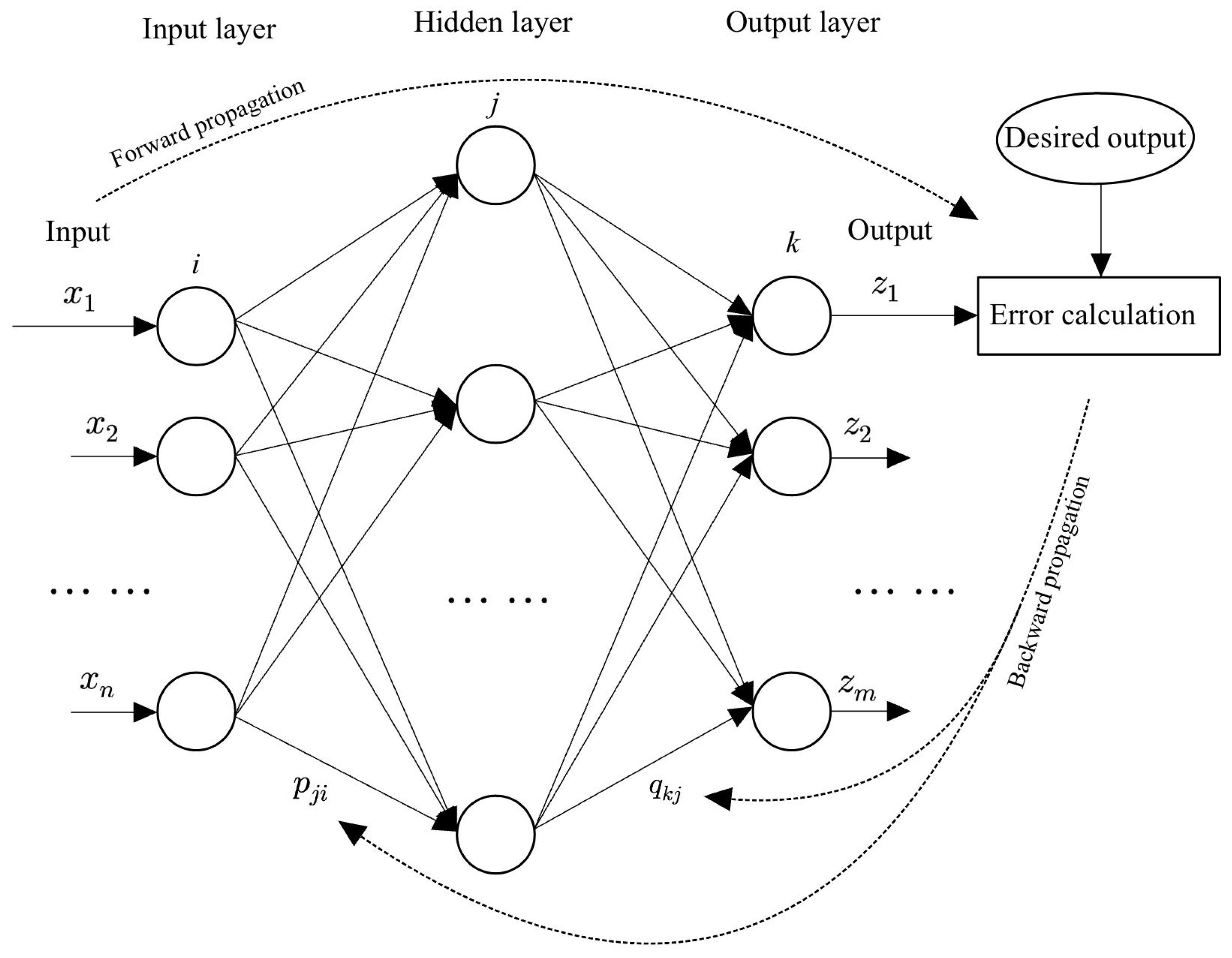
2.1. Network Structure

We employ a three-layer BP neural network structure, as illustrated in Figure 1. In the neural network model, the input layer consists of n neurons, the hidden layer contains h neurons, and the output layer has m neurons. The neural network has both forward propagation and backward propagation. The forward propagation process consists of learning data features of the neural network. For given sample data, let x = ( x 1 , x 2 , , x n ) T be the variable vector of the input layer, y = y 1 , y 2 , , y h T the variable vector of the hidden layer, z = ( z 1 , z 2 , , z m ) T the variable vector of the output layer, and z ^ = z ^ 1 , z ^ 2 , , z ^ m T the desired output. Moreover, let P = p j i be the weight matrix connected with the input layer and the hidden layer, and Q = ( q k j ) the weight matrix connected to the hidden layer and the output layer, where i = 1 , , n , j = 1 , , h , and k = 1 , , m . The input and output of neurons in the j th hidden layer are described by
neth j = i = 1 n p j i x i = P j x
and
y j = f ( neth j )
where P j = p j 1 , p j 2 , , p j n , and f is an activation function. The k th output layer’s input and output are given by
neto k = j = 1 h q k j y j = Q k y
and
z k = f neto k
where Q k = q k 1 , q k 2 , , q k h . Then, in every iteration, we obtain the output result of the neural network. Now, we consider a total of t sample inputs. For the d-th sample input ( d { 1 , , t } ), the neural network model automatically corrects the weight p j i and the weight q k j . The total error equation of the neural network’s performance evaluation is formulated by
E = 1 2 d = 1 t k = 1 m z ^ k z k d 2 = d = 1 t g d neto k d = d = 1 t g d Q k y d
where
g d neto k d = 1 2 k = 1 m z k ^ f neto k d 2
and
y d = f neth 1 d , f neth 2 d , , f neth h d T
The error calculation process above is used as the forward propagation process of the neural network model. Its weight update by gradient descent through the error equation can be regarded as the backpropagation of the neural network. For the k-th output layer’s error E k = 1 2 d = 1 t z ^ k z k d 2 , according to the chain rule, the partial derivative of E k with respect to q k j is given by
E k q k j = d = 1 t E k neto k d neto k d q k j = d = 1 t g d neto k d y j d
Similarly, the partial derivative of E k with respect to p j i is expressed by
E k p j i = d = 1 t g d neto k d q k j f ( neth j d ) x i d
Then, the update functions of the weights q k j and p j i are calculated by
q k j l = q k j l 1 η E k q k j l 1
and
p j i l = p j i l 1 η E k p j i l 1
where l is the iteration number, and η is the learning rate. The neural network’s backward propagation process is implemented by using the updated weights, which will be applied to the next iteration.

2.2. Fractional Parameter Update

We incorporate the fractional derivative parameter update method into the neural network to prevent the neural network from becoming trapped in local optima during the training process [24]. In the existing literature, the Riemann–Liouville fractional derivative, the Caputo fractional derivative, and the Grunwald–Letnikov fractional derivative are the three most commonly used types of fractional-order derivatives.
Definition 1.
The Riemann–Liouville fractional-order derivative of f ( x ) is defined as
D x α a     R L f x = D n ( a D x α n f ( x ) ) = 1 Γ ( n α ) d n d x n a x f ( t ) ( x t ) α n + 1 d t
where α is a positive real number and n is the smallest integer greater than α, and Γ = 0 t z 1 e t d t .
Definition 2.
The Caputo fractional-order derivative of f ( x ) is defined as
D x α a C f ( x ) = 1 Γ ( n α ) a x f ( n ) ( t ) ( x t ) α n + 1 d t = 1 Γ ( n α ) a x ( x t ) α n + 1 f ( t ) d t
where α is a positive real number and n 1 < α < n .
Definition 3.
The Grunwald–Letnikov fractional-order derivative f ( x ) is defined as
D x α a     G L = lim h 0 1 h α k = 0 [ x a h ] ( 1 ) k Γ ( α + 1 ) Γ ( k + 1 ) Γ ( α k + 1 ) f ( x k h )
where α is a positive real number.
We employ Caputo fractional-order differentiation in this paper for the following reasons: (1) Caputo fractional-order differentiation has a more unambiguous physical significance. It can be regarded as performing integer-order differentiation on function f first, followed by integration with a weight. This weight can be viewed as a “memory effect”, in which the function’s value at time x is influenced by its value at time t, with the degree of influence decreasing with the increase in time interval x t  [25]. (2) The Caputo fractional order’s initial point is the same as that for the integer order. We know that the Caputo fractional-order derivative’s initial value problem can be written as f 0 , f 0 , f n 1 0 . These are all integer-order derivatives in those forms. Since the initial values are known and the calculation of complicated fractional-order derivatives is not necessary, this greatly simplifies the problem’s solution [26]. (3) In comparison to the other two definitions of fractional order, the Caputo fractional-order derivative in the application of neural networks greatly reduces the amount of calculation. Meanwhile, it is closer to the integer order, making it more appropriate for neural networks’ error calculation process.
In order to simplify the computational complexity of neural networks, this paper chooses the power function and calculates its fractional derivative. For the power function f ( x ) = ( x a ) p , its n-th derivative is
f ( n ) ( x ) = Γ ( p + 1 ) Γ ( p n + 1 ) ( x a ) p n
Substituting f ( n ) ( x ) into the Caputo derivative definition 2 yields
D x α a C = 1 Γ ( n α ) a x Γ ( p + 1 ) Γ ( p n + 1 ) ( t a ) p n ( x t ) α n + 1 d t
This integral can be further simplified by the properties of the Gamma function. When n = p (in which case p is an integer and p α ), the integration becomes relatively simple. Finally, we obtain a specific form of fractional derivative for the power function used in this paper
d α d x α ( x a ) p = Γ ( p + 1 ) Γ ( p α + 1 ) ( x a ) p α
Therefore, the gradient is calculated by
D q k j α E k = d = 1 t q k j 1 α Γ 2 α g d neto k d y j d
D p j i α E k = d = 1 t p j i 1 α Γ 2 α g d neto k d q k j f ( neth j d ) x i d
Finally, according to Formulas (1)–(18), combining fractional-order gradients and the integer-order gradient, the updated weights of the neural network model are
q k j l = q k j l 1 η E k q k j l 1 + τ D q k j l 1 α E k
p j i l = p j i l 1 η E k p j i l 1 + τ D p j i l 1 α E k
where τ is a parameter greater than zero.

2.3. Algorithms

This subsection will provide the proposed MIFBP neural network (MIFBPNN) algorithms. To further demonstrate the algorithm’s superiority, this paper compares this algorithm to the BP neural network (BPNN) and fractional-order BP neural network (FBPNN) algorithms. These three algorithms are presented in Algorithms 1–3.
Algorithm 1 BPNN
  • Initialize the weight matrices p j i , q k j , and the learning parameter η
  • Compute the l t h error function E k = d = 1 t g d Q k y d
  • Update the weight matrices by q k j l = q k j l 1 η E k q k j l 1 and p j i l = p j i l 1 η E k p j i l 1
  • Check if the total error function E meets the accuracy requirements or l > l max , exit the algorithm; If not, go to step 2.
Algorithm 2 FBPNN
  • Initialize the weight matrices p j i , q k j , the learning parameter η , and the parameter α
  • Compute the l t h error function E k = d = 1 t g d Q k y d
  • Update the weight matrices by q k j l = q k j l 1 η D q k j l 1 α E k and p j i l = p j i l 1 η D p j i l 1 α E k
  • Check if the total error function E meets the accuracy requirements or l > l max , exit the algorithm; If not, go to step 2.
Algorithm 3 MIFBPNN
  • Initialize the weight matrices p j i , q k j , the learning parameter η , and the parameters α and τ
  • Compute the l t h error function E k = d = 1 t g d Q k y d
  • Update the weight matrices by
    q k j l = q k j l 1 η E k q k j l 1 + τ D q k j l 1 α E k
    and
    p j i l = p j i l 1 η E k p j i l 1 + τ D p j i l 1 α E k
  • Check if the total error function E meets the accuracy requirements or l > l max , exit the algorithm; If not, go to step 2.

3. Convergence Analysis

In this section, we will prove the convergence properties of the MIFBPNN. To proceed, we need the following assumptions.
Assumption 1.
The activation function f is a Sigmoid function.
Assumption 2.
The weights q k j and p j i are bounded during the MIFBPNN training process.
Assumption 3.
The learning rate η and the parameter τ are positive numbers and have upper bounds.
We have the following main results.
Theorem 1.
Suppose that the Assumptions (1)–(3) are satisfied, then we conclude that the MIFBPNN is convergent.
Proof of Theorem 1. 
This proof consists of two parts. First, we prove that the error function sequence E l is monotonic. Then we demonstrate that the sequence E l is bounded. To explore the monotonicity of the sequence E l , we compute
E * = E l E l 1 = d = 1 t k = 1 m g d Q k l y d , l g d Q k l 1 y d , l 1
According to the Taylor expansion formula and (21), we obtain
g d Q k l y d , l g d Q k l 1 y d , l 1 = g d Q k l 1 y d , l 1 Q k l y d , l Q k l 1 y d , l 1 + 1 2 g d ε 1 Q k l y d , l Q k l 1 y d , l 1 2
where ε 1 is the Lagrange constant between Q k l y d , l and Q k l 1 y d , l 1 .
Moreover, we see that
Q k l y d , l Q k l 1 y d , l 1 = Q k l y d , l y d , l 1 + Q k l Q k l 1 y d , l 1 = Q k l 1 ξ d l + Δ Q k l ξ d l + Δ Q k l y d , l 1
where Δ Q k l = Q k l Q k l 1 and ξ d l = y d , l y d , l 1
Then, substituting (22) to (21) yields
E * = d = 1 t k = 1 m g d Q k l 1 y d , l 1 Q k l 1 ξ d l + d = 1 t k = 1 m g d Q k l 1 y d , l 1 Δ Q k l ξ d l + d = 1 t k = 1 m g d Q k l 1 y d , l 1 Δ Q k l y d , l 1 + 1 2 d = 1 t k = 1 m g d ε 2 Q k l y d , l Q k l 1 y d , l 1 2
We process Q k l 1 ξ d l according to the Taylor extension formula to obtain
Q k l 1 ξ d l = Q k l 1 y d , l y d , l 1 = j = 1 h q k j l 1 f P j l x d f P j l 1 x d = j = 1 h q k j l 1 f P j l 1 x d Δ P j l x d + 1 2 f ε 2 Δ P j l x d 2
where Δ P j l = P j l P j l 1 and ε 2 is the Lagrange constant between P j l x d and P j l 1 x d . According to (20), (23) and (24), we have
d = 1 t k = 1 m g d Q k l 1 y d , l 1 Q k l 1 ξ d l = d = 1 t k = 1 m j = 1 h i = 1 n g d Q k l 1 y d , l 1 q k j l 1 f P j l 1 x d Δ p j i l x i d + 1 2 d = 1 t k = 1 m j = 1 h g d Q l 1 y d , l 1 q k j l 1 f ε 2 Δ P j l x d 2
where
Δ p j i l = p j i l p j i l 1 = η E k p j i l 1 + τ D p j i l 1 α E k = η p j i l 1 α 1 Γ 2 α + τ D p j i l 1 α E k
For simplicity, we define
φ 1 = d = 1 t k = 1 m j = 1 h i = 1 n g d Q k l 1 y d , l 1 q k j l 1 f P j l 1 x d Δ p j i l x i d
φ 2 = 1 2 d = 1 t k = 1 m j = 1 h g d Q k l 1 y d , l 1 q k j l 1 f ε 2 Δ P j l x d 2
φ 3 = d = 1 t k = 1 m g d Q k l 1 y d , l 1 Δ Q k l ξ d l
φ 4 = d = 1 t k = 1 m g d Q k l 1 y d , l 1 Δ Q k l y d , l 1
φ 5 = 1 2 d = 1 t k = 1 m g d ε 2 Q k l y d , l Q k l 1 y d , l 1 2
From (17), we obtain
d = 1 t g d Q k l 1 y d , l 1 q k j l 1 f P j l 1 x d x i d = p j i l 1 α 1 Γ 2 α D p j i l 1 α E k
Furthermore, it follows from (26), (27) and (32) that
φ 1 = Γ 2 α k = 1 m j = 1 h i = 1 n p j i l 1 α 1 D p j i l 1 α E k Δ p j i l = η Γ 2 α k = 1 m j = 1 h i = 1 n p j i l 1 α 1 D p j i l 1 α E k 2 p j i l 1 α 1 Γ 2 α + τ τ η Γ 2 α k = 1 m j = 1 h i = 1 n p j i l 1 α 1 D p j i l 1 α E k 2 = τ η Γ 2 α k = 1 m j = 1 h p j i l 1 α 1 D P j l 1 α E k 2
where D P j l 1 α E k = ( D p j i l 1 α E k ) 1 × h and
φ 3 1 2 d = 1 t k = 1 m g d Q k l 1 y d , l 1 Δ Q k l 2 + ξ d l 2
By using (2), (3), (18) and (19), we have
d = 1 t g d neto k d y j d = d = 1 t g d Q k l 1 y d , l 1 f P j l x d = q k j l 1 α 1 Γ 2 α D q k j l 1 α E k
and
φ 4 = d = 1 t k = 1 m j = 1 h g d Q k l 1 y d , l 1 y j d , l 1 Δ q k j l = Γ 2 α k = 1 m j = 1 h q k j l 1 α 1 Δ q k j l D q k j l 1 α E k
where
Δ q k j l = q k j l q k j l 1 = η E q k j l 1 + τ D q k j l 1 α E = η q k j l 1 α 1 Γ 2 α + τ D q k j l 1 α E k
Thus, we obtain
φ 4 = η Γ 2 α k = 1 m j = 1 h q k j l 1 α 1 q k j l 1 α 1 Γ 2 α + τ D q k j l 1 α E k 2 τ η Γ 2 α k = 1 m j = 1 h q k j l 1 α 1 D q k j l 1 α E k 2 = τ η Γ 2 α k = 1 m q k j l 1 α 1 D Q k l 1 α E k 2
where D Q k l 1 α E k = ( D q k j l 1 α E k ) 1 × m .
φ 5 = 1 2 g d ε 2 d = 1 t k = 1 m Q k l y d , l Q k l 1 y d , l + Q k l 1 y d , l Q k l 1 y d , l 1 2 = 1 2 g d ε 2 d = 1 t k = 1 m Δ Q k l y d , l + Q k l 1 ξ d l 2 g d ε 2 d = 1 t k = 1 m Δ Q k l 2 y d , l 2 + Q k l 1 2 ξ d l 2
Next, let
A 1 = max sup g d t , sup g d t , sup | g d t | , sup | f x | , sup | f x | ,
A 2 = max x d , 1 d t
A 3 = max Φ ,
where Φ = q k j , p j i represents the vector consisting of all stretched weighted parameters q k j and p j i . Then, we obtain through (33)–(42) that
Δ Q k l 2 2 η 2 A 3 α 1 Γ 2 α 2 + τ 2 ) D Q k l 1 α E k 2
Δ P j l 2 2 η 2 A 3 α 1 Γ 2 α 2 + τ 2 D P j l 1 α E k 2
Δ Φ l 2 Δ Q k l 2 + Δ P j l 2 2 η 2 A 3 α 1 Γ 2 α 2 + τ 2 D Q k l 1 α E k 2 + D P j l 1 α E k 2
Moreover, (24), (43) and (44) imply
ξ d l 2 = y d , l y d , l 1 2 = P j l x d P j l 1 x d 2 = f ε 2 Δ P j l x d 2 A 1 2 A 2 2 Δ P j l 2
Hence, from (27)–(46), we obtain
φ 1 τ η m Γ 2 α A 3 α 1 D P j l 1 α E k 2
φ 2 1 2 D k = 1 m j = 1 h A 1 A 3 g d Q k l 1 y d , l 1 Δ P j l 1 x d 2 1 2 m D A 1 2 A 2 2 A 3 Δ Φ 2
φ 3 1 2 A 1 d = 1 t k = 1 m Δ Q k l 2 + A 1 2 A 2 2 Δ P j l 2 m D 2 A 1 1 + A 1 2 A 2 2 Δ Φ 2
φ 4 τ η m Γ 2 α A 3 α 1 D Q k l 1 α E k 2
φ 5 A 1 d = 1 t k = 1 m h A 1 2 Δ Q k l 2 + A 1 2 A 2 2 A 3 2 Q k l 1 2 m D A 1 h A 1 2 + A 1 2 A 2 2 A 3 2 Δ Φ 2
We note from (45) that
D Q k l 1 α E k 2 + D P j l 1 α E k 2 Δ Φ l 2 2 η 2 A 3 α 1 Γ 2 α 2 + τ 2
So, using (46)–(52), we convert E * into the following:
E * τ η m Γ 2 α A 3 α 1 D Q k l 1 α E k 2 + D P j l 1 α E k 2 + m 1 2 D A 1 2 A 2 2 A 3 + 1 2 D A 1 1 + A 1 2 A 2 2 + D A 1 A 1 2 + A 1 2 A 2 2 A 3 2 Δ Φ 2 1 2 η τ m Γ 2 α A 3 α 1 A 3 α 1 Γ 2 α 2 + τ 2 Δ Φ 2 + m 1 2 D A 1 2 A 2 2 A 3 + 1 2 D A 1 1 + A 1 2 A 2 2 + D A 1 h A 1 2 + A 1 2 A 2 2 A 3 2 Δ Φ 2 1 2 η τ m Γ 2 α A 3 α 1 2 τ Γ 2 α A 3 α 1 Δ Φ 2 + m 1 2 D A 1 2 A 2 2 A 3 + 1 2 D A 1 1 + A 1 2 A 2 2 + D A 1 h A 1 2 + A 1 2 A 2 2 A 3 2 Δ Φ 2 1 4 η Δ Φ 2 + 1 2 D A 1 2 A 2 2 A 3 + 1 2 D A 1 1 + A 1 2 A 2 2 + D A 1 h A 1 2 + A 1 2 A 2 2 A 3 2 Δ Φ 2
Therefore, the error function sequence E l is monotonically decreasing. Next, since
1 4 η 1 2 D A 1 2 A 2 2 A 3 + 1 2 D A 1 1 + A 1 2 A 2 2 + D A 1 h A 1 2 + A 1 2 A 2 2 A 3 2
then, we obtain the learning rate
η 1 2 D A 1 2 A 2 2 A 3 + 2 D A 1 1 + A 1 2 A 2 2 + 4 D A 1 h A 1 2 + A 1 2 A 2 2 A 3 2
Now, we start to prove the above sequence is also bounded. Let
δ l 1 = D Q k l 1 α E k 2 + D P j l 1 α E k 2
According to (53)–(56) we obtain
E * ( τ η m Γ 2 α A 3 α 1 2 η 2 m A 3 α 1 Γ 2 α + τ 2 ( 1 2 D A 1 2 A 2 2 A 3 + 1 2 D A 1 1 + A 1 2 A 2 2 + D A 1 h A 1 2 + A 1 2 A 2 2 A 3 2 ) ) δ l 1 ( τ η Γ 2 α A 3 α 1 4 τ η 2 Γ 2 α A 3 α 1 ( 1 2 D A 1 2 A 2 2 A 3 + 1 2 D A 1 1 + A 1 2 A 2 2 + D A 1 h A 1 2 + A 1 2 A 2 2 A 3 2 ) ) δ l 1 ρ δ l 1
where
ρ = τ η Γ 2 α A 3 α 1 4 τ η 2 Γ 2 α A 3 α 1 1 2 D A 1 2 A 2 2 A 3 + 1 2 D A 1 1 + A 1 2 A 2 2 + D A 1 h A 1 2 + A 1 2 A 2 2 A 3 2
From (57), we infer that
0 E l E l 1 ρ δ l 1 E l 2 ρ δ l 2 ρ δ l 1 E l 3 ρ δ l 3 ρ δ l 2 ρ δ l 1 E 0 ρ w = 0 l 1 δ w
Then,
w = 0 l 1 δ w 1 ρ E 0
When l , we have w = 0 δ w 1 ρ E 0 < and lim l δ l = 0 . Therefore, according to (57)–(59) the sequence E l is bounded. Using the monotone convergence theorem, we conclude that the sequence E l converges. □

4. Numerical Experiments

4.1. Experiment Preparation

In this section, we use the MNIST handwritten dataset to evaluate the efficiency of the MIFBPNN. We also use BPNN and FBPNN to perform comparison experiments. The MNIST handwritten digit dataset contains 70,000 handwritten digit images ranging from 0 to 9, each with a size of 28 × 28 pixels, represented as a 784 × 1 vector. Each element in the vector takes values ranging from 0 to 255. We first build a 784-50-10 neural network model ( n = 784 , h = 30 , m = 10 ) based on the characteristics of the MNIST data, and in our experiments, we found that when the number of hidden layers is 50, we could achieve high accuracy in the test set, which greatly reduces the computational amount of the neural network model. The activation function uses the Sigmoid function, which is expressed as f x = 1 1 + e x . Then, we divided the dataset into 60,000 handwritten images to use as the training set, and the remaining 10,000 sets of data to use as the test set. As the convergence of the neural network does not mean that the network has completely learned all the features and patterns of the dataset, but rather that the network has reached a relatively stable state, in order to study this stable state, in the experiments of this paper, we set the condition: When the accuracy of the test set of every 10 epochs grows no more than 0.001, then exit the training. In this way, it is possible to determine whether the neural network has reached a stable state based on the number of epochs, and thus better evaluate the neural network. (The experimental platform for these experiments was a PC running Windows OS, with an i7-11657G7 CPU and M40 GPU).

4.2. Optimal Parameters Tuning

In the experiment, we set the same parameters for each model to more effectively compare the three models used in this paper. There are three parameters in the proposed MIFBPNN. We first determined η = 0.7 and α = 0.6 based on the BP neural network training result in Table 1 and the training result of the FBPNN in Table 2. Based on the training outcomes of the MIFBPNN in Table 3, we discovered τ = 0.2 .
Table 1, Table 2 and Table 3 show that the MIFBPNN achieves a stable state faster and has a higher accuracy rate than the FBPNN and BPNN, which may suggest that the MIFBPNN is able to learn better under the same circumstances.

4.3. Training for Different Training Sets’ Sizes

A larger training set can provide more sample data for the model to learn from, which can help to improve the accuracy and generalizability of the model. Typically, the size of the training set can have an impact on the training results. Here, we investigate the performance of the three neural networks by adjusting various training set sizes, and the experimental results are displayed in Table 4, which shows that a larger training set can aid the model in better-capturing patterns and features from the data.
Table 4 shows that, in terms of training accuracy and the number of layers to stop training, the MIFBPNN performs best on training datasets of all sizes, followed by the FBPNN. It is worth noting that change in the MIFBPNN’s accuracy from the training dataset of 10,000 to 60,000 was the smallest, followed by that of the FBPNN. This can also be viewed as evidence that the MIFBPNN is more general and has a stronger capacity for convergence and learning while maintaining high accuracy.

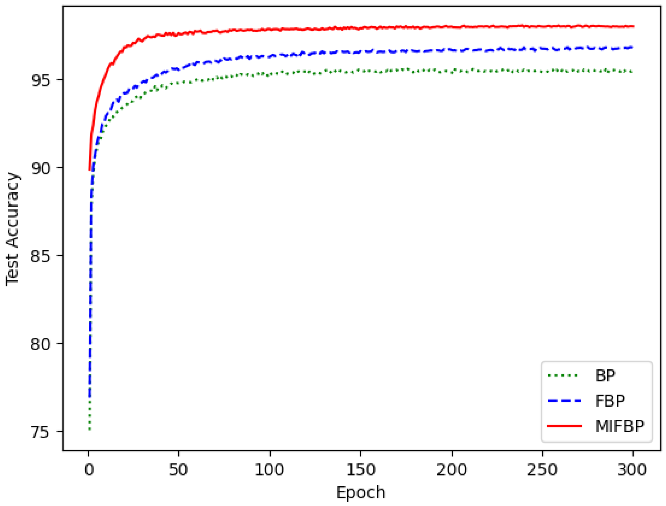
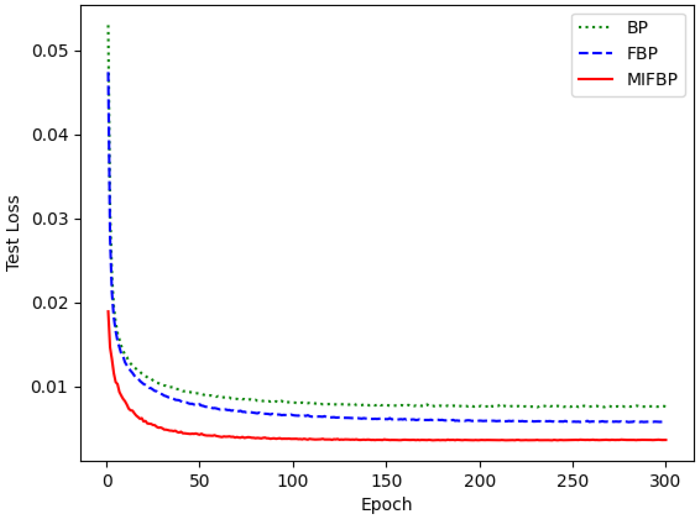
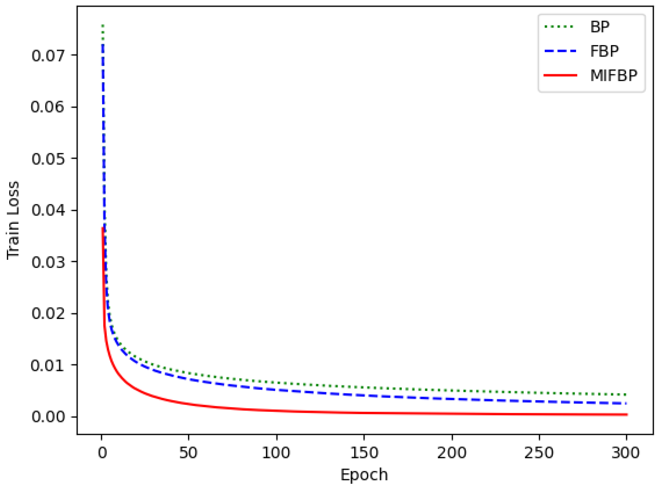
4.4. Training Performances of Different Neural Networks

In this subsection, we demonstrate the performance of the three neural networks using the optimal parameters and a training dataset of 60,000. Figure 2 and Figure 3 depict the three neural networks’ test accuracy and test set loss performance, respectively, and Figure 4 depicts the three neural networks’ training set loss performance.
The MIFBPNN has the highest accuracy, followed by the FBPNN, as can be seen in Figure 3. In terms of convergence speed, the accuracy of the MIFBPNN and FBPNN reaches a relatively stable state in about 50 and 80 epochs, while the BP neural network experiences this process in about 120 epochs. The MIFBPNN has the smallest loss and can reach the minimum loss fastest, both in the training set loss and the test set loss, as shown by Figure 3 and Figure 4.
Based on the above experimental results, it can be concluded that MIFBPNN exhibits high accuracy and fast convergence speed in various training set sizes under different experimental conditions. Especially on the maximum size training set (60,000 samples), the MIFBPNN not only achieved the highest accuracy (97.64%) but also had lower training epoch (71 epochs) than the other two networks, demonstrating its excellent learning ability and generalization ability. Furthermore, from the chart analysis, it can be seen that the MIFBPNN outperforms BPNN and FBPNN in terms of testing accuracy, testing loss, and training loss. Especially in terms of minimizing losses, MIFBP networks can achieve lower loss values faster, which is of great significance for optimizing and improving efficiency in practical applications. Secondly, the MIFBPNN also demonstrated its superiority in parameter adjustment experiments. After fixing η = 0.7 and α = 0.6 , and adjusting the τ parameters, it is found that the network performed best at τ = 0.2 , with an accuracy of 97.64%. This result not only demonstrates the advantage of MIFBPNN in parameter sensitivity but also highlights its adjustment flexibility and efficiency in practical applications. However, the limitation of this article is that it only applies the MIF algorithm to BPNN, and manual adjustments are used during the parameter adjustment process. In future work, attempts can be made to apply the MIF algorithm to other neural networks, and heuristic algorithms can be considered when adjusting parameters α , η , and τ . Furthermore, the computational effort of the MIFBPNN is not explained in this article. These issues are worth exploring in future work.

5. Conclusions

In this paper, we develop a new MIF gradient descent algorithm to construct the MIFBP neural network. Our research demonstrates the MIFBP neural network’s superior performance on the typical MNIST handwritten dataset. For various training set sizes, the MIFBP network outperforms conventional BP and FBPNN in terms of accuracy, convergence speed, and generalization. Additionally, in both training and testing scenarios, the MIFBPNN achieves the highest accuracy and the lowest loss under optimal parameter conditions. The MIFBPNN has shown good classification performance in the MNIST handwritten data and may perform challenging pattern recognition and prediction tasks in various fields in the future.

Author Contributions

Y.Z.: conceptualization, methodology, software, validation, formal analysis, investigation, and writing—original draft preparation. H.X.: conceptualization, methodology, writing—review and editing, supervision, and funding acquisition. Y.L.: methodology, project administration, and funding acquisition. G.L.: writing—review and editing, and validation. L.Z.: methodology, formal analysis, and investigation. C.T.: methodology, software, and validation. Y.W.: conceptualization and supervision. All authors have read and agreed to the published version of the manuscript.

Funding

This research was funded an Australian Research Council linkage grant (LP160100528), an innovative connection grant (ICG002517), and an industry grant (SE67504).

Data Availability Statement

The raw data supporting the conclusions of this article will be made available by the authors on request.

Conflicts of Interest

The authors declare no conflict of interest.

References

  1. Edwards, C.J. The Historical Development of the Calculus; Springer Science & Business Media: Berlin/Heidelberg, Germany, 2012. [Google Scholar]
  2. Oldham, K.; Spanier, J. The Fractional Calculus Theory and Applications of Differentiation and Integration to Arbitrary Order; Academic Press: Cambridge, MA, USA, 1974. [Google Scholar]
  3. Hahn, D.W.; Özisik, M.N. Heat Conduction; John Wiley & Sons: Hoboken, NJ, USA, 2012. [Google Scholar]
  4. Matlob, M.A.; Jamali, Y. The concepts and applications of fractional order differential calculus in modeling of viscoelastic systems: A primer. Crit. Rev. Biomed. Eng. 2019, 47, 249–276. [Google Scholar] [CrossRef] [PubMed]
  5. Dehestani, H.; Ordokhani, Y.; Razzaghi, M. Fractional-order Legendre–Laguerre functions and their applications in fractional partial differential equations. Appl. Math. Comput. 2018, 336, 433–453. [Google Scholar] [CrossRef]
  6. Yuxiao, K.; Shuhua, M.; Yonghong, Z. Variable order fractional grey model and its application. Appl. Math. Model. 2021, 97, 619–635. [Google Scholar] [CrossRef]
  7. Kuang, Z.; Sun, L.; Gao, H.; Tomizuka, M. Practical fractional-order variable-gain supertwisting control with application to wafer stages of photolithography systems. IEEE/ASME Trans. Mechatronics 2021, 27, 214–224. [Google Scholar] [CrossRef]
  8. Liu, C.; Yi, X.; Feng, Y. Modelling and parameter identification for a two-stage fractional dynamical system in microbial batch process. Nonlinear Anal. Model. Control 2022, 27, 350–367. [Google Scholar] [CrossRef]
  9. Wang, S.; Li, W.; Liu, C. On necessary optimality conditions and exact penalization for a constrained fractional optimal control problem. Optim. Control Appl. Methods 2022, 43, 1096–1108. [Google Scholar] [CrossRef]
  10. Bhrawy, A.H.; Ezz-Eldien, S.S.; Doha, E.H.; Abdelkawy, M.A.; Baleanu, D. Solving fractional optimal control problems within a Chebyshev–Legendre operational technique. Int. J. Control 2017, 90, 1230–1244. [Google Scholar] [CrossRef]
  11. Saxena, S. Load frequency control strategy via fractional-order controller and reduced-order modeling. Int. J. Electr. Power Energy Syst. 2019, 104, 603–614. [Google Scholar] [CrossRef]
  12. Mohammadi, H.; Kumar, S.; Rezapour, S.; Etemad, S. A theoretical study of the Caputo–Fabrizio fractional modeling for hearing loss due to Mumps virus with optimal control. Chaos Solitons Fractals 2021, 144, 110668. [Google Scholar] [CrossRef]
  13. Aldrich, C. Exploratory Analysis of Metallurgical Process Data with Neural Networks and Related Methods; Elsevier: Amsterdam, The Netherlands, 2002. [Google Scholar]
  14. Bhattacharya, U.; Parui, S.K. Self-adaptive learning rates in backpropagation algorithm improve its function approximation performance. In Proceedings of the ICNN’95-International Conference on Neural Networks, Perth, WA, Australia, 27 November–1 December 1995; IEEE: Piscataway, NJ, USA, 1995; Volume 5, pp. 2784–2788. [Google Scholar]
  15. Niu, H.; Chen, Y.; West, B.J. Why do big data and machine learning entail the fractional dynamics? Entropy 2021, 23, 297. [Google Scholar] [CrossRef]
  16. Xu, C.; Liao, M.; Li, P.; Guo, Y.; Xiao, Q.; Yuan, S. Influence of multiple time delays on bifurcation of fractional-order neural networks. Appl. Math. Comput. 2019, 361, 565–582. [Google Scholar] [CrossRef]
  17. Pakdaman, M.; Ahmadian, A.; Effati, S.; Salahshour, S.; Baleanu, D. Solving differential equations of fractional order using an optimization technique based on training artificial neural network. Appl. Math. Comput. 2017, 293, 81–95. [Google Scholar] [CrossRef]
  18. Asgharnia, A.; Jamali, A.; Shahnazi, R.; Maheri, A. Load mitigation of a class of 5-MW wind turbine with RBF neural network based fractional-order PID controller. ISA Trans. 2020, 96, 272–286. [Google Scholar] [CrossRef] [PubMed]
  19. Fei, J.; Wang, H.; Fang, Y. Novel neural network fractional-order sliding-mode control with application to active power filter. IEEE Trans. Syst. Man Cybern. Syst. 2021, 52, 3508–3518. [Google Scholar] [CrossRef]
  20. Zhang, Y.; Xiao, M.; Cao, J.; Zheng, W.X. Dynamical bifurcation of large-scale-delayed fractional-order neural networks with hub structure and multiple rings. IEEE Trans. Syst. Man Cybern. Syst. 2020, 52, 1731–1743. [Google Scholar] [CrossRef]
  21. Cao, J.; Stamov, G.; Stamova, I.; Simeonov, S. Almost periodicity in impulsive fractional-order reaction–diffusion neural networks with time-varying delays. IEEE Trans. Cybern. 2020, 51, 151–161. [Google Scholar] [CrossRef] [PubMed]
  22. Bao, C.; Pu, Y.; Zhang, Y. Fractional-order deep backpropagation neural network. Comput. Intell. Neurosci. 2018, 2018, 7361628. [Google Scholar] [CrossRef] [PubMed]
  23. Han, X.; Dong, J. Applications of fractional gradient descent method with adaptive momentum in BP neural networks. Appl. Math. Comput. 2023, 448, 127944. [Google Scholar] [CrossRef]
  24. Prasad, K.; Krushna, B. Positive solutions to iterative systems of fractional order three-point boundary value problems with Riemann–Liouville derivative. Fract. Differ. Calc. 2015, 5, 137–150. [Google Scholar] [CrossRef]
  25. Hymavathi, M.; Ibrahim, T.F.; Ali, M.S.; Stamov, G.; Stamova, I.; Younis, B.; Osman, K.I. Synchronization of fractional-order neural networks with time delays and reaction-diffusion terms via pinning control. Mathematics 2022, 10, 3916. [Google Scholar] [CrossRef]
  26. Wu, Z.; Zhang, X.; Wang, J.; Zeng, X. Applications of fractional differentiation matrices in solving Caputo fractional differential equations. Fractal Fract. 2023, 7, 374. [Google Scholar] [CrossRef]
Figure 1. A three-layer BP neural network architecture.
Algorithms 17 00220 g001
Figure 2. Test accuracy performance.
Algorithms 17 00220 g002
Figure 3. Test loss performance.
Algorithms 17 00220 g003
Figure 4. Training loss performance.
Algorithms 17 00220 g004
Table 1. Test set accuracy of the BP neural network with various parameter values of η .
η = 0.1 η = 0.2 η = 0.3 η = 0.4 η = 0.5 η = 0.6 η = 0.7 η = 0.8 η = 0.9
Accuracy93.79%94.15%94.50%95.20%95.22%95.30%95.65%95.60%95.45%
Training epoch246297245257217191163197203
Table 2. Test set accuracy of the FBPNN with η = 0.7 and various parameter values of α .
η = 0.7 α = 0.1 α = 0.2 α = 0.3 α = 0.4 α = 0.5 α = 0.6 α = 0.7 α = 0.8 α = 0.9
Accuracy96.28%95.86%95.87%95.76%96.01%96.65%96.13%95.93%95.70%
Training epoch797555637068677357
Table 3. Test set accuracy of the MIFBPNN with η = 0.7 , α = 0.6 and various parameter values of τ .
η = 0.7 , α = 0.6 τ = 0.1 τ = 0.2 τ = 0.3 τ = 0.4 τ = 0.5 τ = 0.6 τ = 0.7 τ = 0.8 τ = 0.9
Accuracy97.52%97.64%97.34%97.30%97.27%97.41%97.46%97.49%97.36%
Training epoch637154555051475655
Table 4. Performance of different neural networks under optimal hyperparameters on various sizes of training sets.
Training Dataset SizeBPFBPMIFBP
Accuracy Training Epoch Accuracy Training Epoch Accuracy Training Epoch
10,00091.69%12492.99%8694.55%79
20,00093.71%17693.29%7696.06%64
30,00093.81%14093.85%6896.94%69
40,00094.20%10994.23%5897.17%55
50,00095.23%15795.69%7197.28%61
60,00095.65%16396.95%6897.64%71
Disclaimer/Publisher’s Note: The statements, opinions and data contained in all publications are solely those of the individual author(s) and contributor(s) and not of MDPI and/or the editor(s). MDPI and/or the editor(s) disclaim responsibility for any injury to people or property resulting from any ideas, methods, instructions or products referred to in the content.

