Abstract
Facial emotion recognition (FER) is crucial across psychology, neuroscience, computer vision, and machine learning due to the diversified and subjective nature of emotions, varying considerably across individuals, cultures, and contexts. This study explored FER through convolutional neural networks (CNNs) and Histogram Equalization techniques. It investigated the impact of histogram equalization, data augmentation, and various model optimization strategies on FER accuracy across different datasets like KDEF, CK+, and FER2013. Using pre-trained VGG architectures, such as VGG19 and VGG16, this study also examined the effectiveness of fine-tuning hyperparameters and implementing different learning rate schedulers. The evaluation encompassed diverse metrics including accuracy, Area Under the Receiver Operating Characteristic Curve (AUC-ROC), Area Under the Precision–Recall Curve (AUC-PRC), and Weighted F1 score. Notably, the fine-tuned VGG architecture demonstrated a state-of-the-art performance compared to conventional transfer learning models and achieved 100%, 95.92%, and 69.65% on the CK+, KDEF, and FER2013 datasets, respectively.
1. Introduction
Emotions play a significant role in human interactions, serving as essential mediators in social communication systems [1]. Humans’ expression of emotions incorporates diverse modalities, including facial expressions, speech patterns [2], and body language [3]. According to Darwin and Prodger [4], human facial expressions indicate humans’ emotional states and intentions. Recently, automatic emotion detection through computer vision techniques has shown a growth in interest and application across many domains, including hospital patient care [5], neuroscience research [6], smart home technologies [7], and even in cancer treatment [8,9]. This diversity has established emotion recognition as a distinct and growing field in research fields, primarily due to its wide range of applications and intense impact on various phases of human life.
Emotion recognition from images mainly consists of two steps: feature extraction and classification. Facial images encompass a multitude of features including geometric, texture, color, intensity, landmark, shape, and histogram-based features. Handcrafted techniques for feature extraction in facial images involve the manual identification of landmarks for geometric features, texture analysis using methods like Local Binary Patterns (LBPs) [10], and color distribution analysis through histograms. To enhance the feature extraction process, dimensionality reduction techniques such as PCA (Principal Component Analysis) [11]/t-SNE (t-Distributed Stochastic Neighbor Embedding) [12] have been employed to obtain crucial features for classification. Traditional machine learning algorithms like Support Vector Machine (SVM) [13] and Random Forest (RF) [14] have been used to classify the emotions from these features. However, hand-crafted features often struggle to capture the important information required for effective face identification. Moreover, kernel-based methods frequently produce feature vectors that are excessively large, leading to the overfitting of the model [15].
Deep learning models, particularly convolutional neural networks (CNNs) [16], are renowned for their capability to automatically learn hierarchical features and complex patterns. However, CNNs frequently face challenges such as overfitting, which arises from limited data availability and computational complexity. Additionally, issues like vanishing or exploding gradients can undermine the stability of the training processes [17].
Transfer learning has gained popularity in machine learning as a method for accelerating tasks. Transfer learning provides a framework for leveraging well-known pre-trained models, such as VGG (Visual Geometry Group) [18], ResNet [19], and DenseNet121 [20], trained on millions of image data and is particularly relevant for FER application in the related domain of facial images.
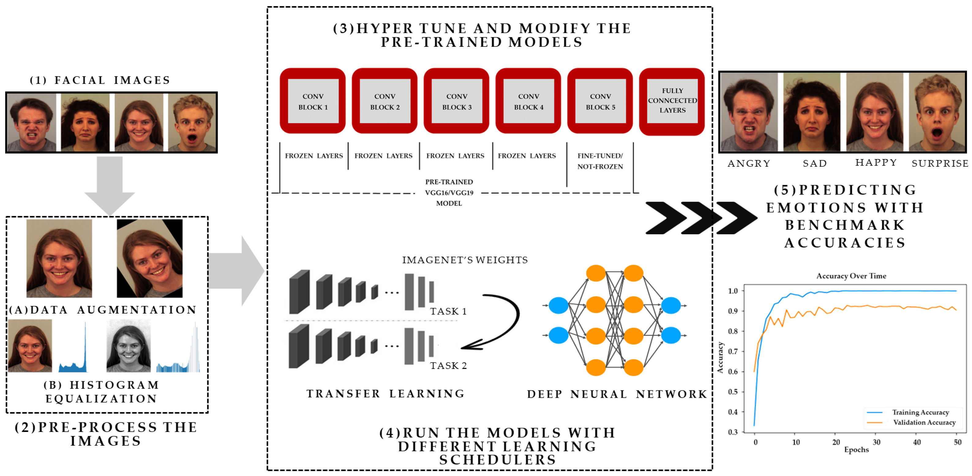
A schematic representation of the proposed framework is presented in Figure 1, utilizing images sourced from the Karolinska Directed Emotional Faces (KDEF) [21] dataset for illustrative purposes. As presented in Figure 1, the first step (1) showcases facial images retrieved from the KDEF, Filtered Facial Expression Recognition 2013 (FER2013) [22], and Cohn-Kanade (CK+) [23] datasets. In the subsequent step, step (2), the data undergo preprocessing, wherein data augmentation techniques such as horizontal flipping, zooming, rotation, and histogram equalization [24] methods are applied. These techniques serve to augment the dataset, enhancing image contrast and thereby facilitating improved feature extraction. In moving forward to step (3), the fine-tuning and modification of the pre-trained VGG19 and VGG16 models are undertaken. During this process, the last convolutional block of the models is kept unfrozen, while the remaining layers of the base models (pre-trained VGG16, VGG19) are frozen. Additionally, the fully connected layers are then connected to these models. Moreover, diverse learning rate schedulers, including cosine annealing [25] are implemented in the models. The evaluation phase encompasses training the models on datasets such as KDEF, Filtered FER2013, and CK+, followed by an assessment using various evaluation metrics. These metrics include the accuracy, AUC-ROC [26], AUC-PRC, and Weighted F1 score [27].

Figure 1.
The overall workflow of the proposed framework.
A significant contribution of this study is on optimizing the performance of a pre-trained simple architecture such as a VGG on well-known FER image datasets. Instead of opting for complex deep neural network models, this study demonstrates that careful fine-tuning can lead to better classification accuracy with simpler architectures. This study investigated the efficacy of histogram equalization and data augmentation in improving the FER accuracy, alongside optimizing the performances of pre-trained architectures like VGG on three benchmark FER datasets. Additionally, this study showcases the effectiveness of different regularization techniques, callbacks, and learning schedulers in enhancing the model performance for FER by conducting extensive experiments.
The subsequent sections of this paper are structured as follows. Section 2 presents a review of the related literature in the field. Section 3 introduces histogram equalization and cosine annealing to aid in understanding the proposed models. Section 4 elaborates on the transfer learning-based model, datasets used, and the experiment pipeline. Section 5 presents the experimental results, while Section 6 provides a thorough discussion of these results. Finally, Section 7 concludes this paper by discussing its significance and outlining potential future work.
2. Related Works
Numerous studies conducted in recent years have focused on FER, employing various techniques. Traditional machine learning approaches have been used alongside CNN models to obtain important information for classifying emotions extracted from visual objects.
Xiao-Xu et al. [28] employed an ensemble approach using Wavelet Energy Features (WEFs) and Fisher’s Linear Discriminants (FLD) for the feature extraction and classification of seven facial expressions (anger, disgust, fear, happiness, neutral, sadness, surprise) within the Japanese Female Facial Expression (JAFFE) dataset [29]. Abhinav Dhall et al. utilized the Pyramid of Histogram of Gradients (PHOG) [30] and Local Phase Quantization (LPQ) [31] features to encode shape and appearance information. They selected keyframes through the K-means clustering [32] of normalized shape vectors from Constrained Local Models (CLMs) based face tracking. Emotion classification on the SSPNET [33] and GEMEP-FERA [34] datasets was conducted using an SVM and the Largest Margin Nearest Neighbor (LMNN) algorithm [35]. Pu et al. proposed a framework employing two-fold RF classifiers to recognize Action Units (AUs) from image sequences. Facial motion measurements involved tracking Active Appearance Model (AAM) [36] facial feature points with Lucas–Kanade optical flow [37], using displacement vectors between the neutral and peak expressions as motion features. These features were fed into a first-level RF for AU determination, followed by a second-level RF for facial expression classification [38]. Golzadeh et al. focused on spatio-temporal feature extraction based on tracked facial landmarks, aiming to develop an automatic emotion recognition system [39]. They employed the KDEF dataset to identify features that represent different human facial expressions, subsequently evaluating them through various classification methods. Through experimentation and employing K-fold cross-validation, they achieved the precise recognition of facial expressions, attaining up to 87% accuracy with the newly devised features and a multiclass SVM classifier. Liew et al. proposed five feature characteristics for FER and compared their performances using different classifiers and datasets (KDEF, CK+, JAFFE, and MUG [40]). Among Gaussian-based filtering and response (GABOR) methods, Haar [41], LBP, and histogram of oriented gradients (HOG) [42] classifiers, HOG classifiers perform best for FER with higher image resolutions (above 48 × 48 pixels), averaging an 80% accuracy in these datasets [43].
The researchers found that the most straightforward method for classifying emotions is through CNN models. CNNs are well suited for image tasks due to their ability to capture various levels of features efficiently and recognize patterns and objects in images regardless of their positions or sizes. Thakare et al. used several classifiers such as ConvNet, RF classifiers, and Extreme Gradient Boosting (XGBoost) classifiers [44], with the CNN model ConvNet consistently yielding the highest accuracy in emotion classification [45]. The researchers proposed a novel FER approach that integrates a CNN with image edge detection to bypass traditional feature extraction. This method involves normalizing facial images, extracting edges, and merging this information with features to preserve the structural composition. Subsequently, implicit features are reduced using maximum pooling, followed by a softmax classification for emotion recognition. Testing on the FER2013 [46] and LFW datasets [47] resulted in an average emotion detection rate of 88.56% with faster training, approximately 1.5 times quicker than comparative models [48]. Badrulhisham et al. focused on real-time FER, employing MobileNet [49] to train their model, achieving an 85% recognition accuracy for four emotions (happy, sad, surprise, disgust) on their custom dataset [50]. Experimental validation across multiple databases and facial orientations resulted in significant findings: achieving an accuracy of 89.58% on the KDEF dataset, 100% accuracy on the JAFFE dataset, and 71.975% accuracy on the combined dataset (KDEF + JAFFE + SFEW). These results were obtained using cross-validation techniques to minimize bias.
In [51], researchers explored visual emotion recognition through social media images by employing pre-trained VGG19, ResNet50V2, and DenseNet-121 architectures as their base. Through fine-tuning and regularization techniques, these models demonstrated improved performances on Twitter images from the Crowdflower dataset, with DenseNet-121 exhibiting superior accuracies of 73%, 75%, and 89%, respectively. Furthermore, Subudhiray et al. investigated dual transfer learning for facial emotion classification, experimenting with pre-trained CNN architectures including VGG16, ResNet50, Inception ResNet [52], Wide ResNet [53], and AlexNet. By combining extracted feature vectors into various pairs and inputting them into an SVM classifier, this approach showed promising results in terms of accuracy, kappa, and overall accuracy compared to state-of-the-art methods across benchmark datasets such as JAFFE, CK+, KDEF, and FER2013 [54]. Kaur et al. introduce FERFM, a novel approach using a fine-tuned MobileNetV2 [55] for FER on mobile devices. A pipeline strategy was introduced, where the pre-trained MobileNetV2 architecture is fine-tuned by eliminating the last six layers and adding a dropout, max pooling, and dense layer. Using transfer learning from ImageNet, the method achieved an accuracy of 85.7% on the RGB-KDEF dataset. It surpasses VGG16 with faster processing at 43 ms per image and fewer trainable parameters, totaling 1,510,599 [56]. In another research, they proposed a system that employs a CNN framework using AlexNet’s features, achieving higher accuracy compared to other methods across various datasets like JAFFE, KDEF, CK+, FER2013, and AffectNet [57]. Moreover, they proved it is more efficient and requires fewer device resources than other state-of-the-art deep learning models like VGG16, GoogleNet [58], and ResNet [59]. In another study, Zavarez et al. fine-tuned the VGG-Face Deep CNN model pre-trained for face recognition. The study investigated the impact of a cross-database approach [60]. The results revealed significant accuracy improvements, with average accuracies of 88.58%, 67.03%, 85.97%, and 72.55% on the CK+, MMI, RaFD, and KDEF databases, respectively.
Puthanidam et al. proposed a hybrid facial expression recognition model combining image pre-processing and convolutional neural network (CNN) structures to enhance accuracy and reduce training time. Across various databases and facial orientations, the model achieved high accuracies, with notable results, including 100% accuracy for the JAFFE dataset and 89.58% accuracy for the KDEF dataset [61]. Chen et al. introduced the Attentive Cascaded Network (ACD) method, which enhances the discriminative power of facial expression recognition models by selectively focusing on important feature elements [62]. By integrating multiple feature extractors with smooth center loss, ACD achieves intra-class compactness and inter-class separation, improving the generalization ability of the learning algorithm. In their experiment, the proposed method achieved a notable performance on the RAF-DB and KDEF datasets, with accuracies of 86.42% and 99.12%, respectively. In [63], the researchers introduced a novel approach to facial expression recognition by combining deep metric loss and softmax loss in a unified framework, enhancing the performance by addressing intra- and inter-class variations. Using a generalized adaptive (N+M)-tuplet cluster loss function and identity-aware mining schemes, the proposed method achieved an accuracy of approximately 97.1% on the CK+ dataset and 78.53% on the MMI dataset [64]. Dar et al. used EfficientNet-b0 for feature extraction and transfer learning due to its accuracy and computational efficiency balance [65]. They customized the EfficientNet-b0 architecture by incorporating Swish activation functions after every 2D convolution layer, enhancing performance through non-monotonic, smooth unbounded above/bounded below properties. The researchers assessed the effectiveness of their model across five varied datasets: CK+, JAFFE, FER-2013, KDEF, and FERG. They reported classification accuracies of 100%, 95.02%, 63.4%, 88.3%, and 100% respectively for these datasets. Zahara et al. proposed a system design that utilizes convolutional neural networks (CNNs) with the OpenCV library to predict and classify facial emotions in real time [66]. Implemented on Raspberry Pi, the system comprises three main processes: face detection, facial feature extraction, and emotion classification. The Xception model achieved a prediction accuracy of 65.97% on the FER-2013 dataset for facial expression recognition. Minaee et al. introduced a deep learning approach employing attentional convolutional networks for facial expression recognition, surpassing previous models on various datasets, including FER-2013, CK+, FERG, and JAFFE, achieving accuracies of 70.02%, 98%, 99.3%, and 92.8%, respectively [67]. Fie et al. introduced a novel deep neural network-based system for the early detection of cognitive impairment by analyzing the evolution of facial emotions in response to video stimuli. The system incorporates a facial expression recognition algorithm using layers from MobileNet and a Support Vector Machine (SVM), demonstrating satisfactory performances across three datasets like the KDEF dataset, Chinese Adults Dataset, and Chinese Elderly People Dataset [68]. A significant amount of work has focused on employing transfer learning techniques with CNN models such as AlexNet [69], SqueezeNet [70], and VGG19, evaluating their efficacy on benchmark datasets including FER2013, JAFFE, KDEF, CK+, SFEW [71], and KMU-FED. VGG19 demonstrated a notable performance, achieving 99.7% accuracy on the KMU-FED database and competitive results across other benchmark datasets. Specifically, VGG19 attained performance accuracies of 98.98% for the CK+ dataset, 92.99% for the KDEF dataset with all data variations, 91.5% for the selected KDEF Frontal View dataset, 84.38% for JAFFE, 66.58% for FER2013, and 56.02% for SFEW [72]. Bialek et al. explored emotion recognition through convolutional neural networks (CNNs), proposing various models including custom and transfer learning types, as well as ensemble approaches, alongside FER2013 dataset modifications. Emotion classification has been examined using both multi-class and binary approaches, with results and comparative analyses provided for the different methods and models [22]. In [73], the authors proposed a method for facial expression recognition by concatenating spatial pyramid Zernike moment-based shape features with Law’s texture features, capturing both macro and micro details of facial expressions. Using multilayer perceptron (MLP) and radial basis function feed-forward artificial neural networks, the method achieved a high recognition accuracy, with average rates of 95.86% and 88.87% on the JAFFE and KDEF datasets, respectively.
3. Methodology
In this section, we briefly review the histogram equalization technique and introduce the cosine annealing strategy and evaluation metrics used in this work.
3.1. Histogram Equalization
Histogram equalization is a technique used in image processing to enhance the contrast and improve the overall appearance of an image by redistributing the intensity values across the image. Dark and light regions in an image might not have optimal contrast, making details hard to perceive. Histogram equalization spreads out the intensity levels, making darker areas darker and brighter areas brighter.
The histogram of a digital image with intensity levels in the range [0, L − 1] is a discrete function = , where L is the number of the level, is the kth intensity value, and is the number of pixels in the image with intensity . It is common practice to normalize a histogram by dividing each of its components by the total number of pixels in the image, which is denoted by M × N, where M and N are the row and column dimensions of the image. A normalized histogram is given by
where can be seen as an estimate of the probability of the occurrence of intensity level , in an image. Then,
Consider the continuous intensity values and let the variable r denote the intensities of an image. We assume that r is in the range [0, L − 1]. We focus on transformations (intensity mappings) of the form s = T(r), where , which produces an output intensity level s for every pixel in the input image with intensity [74].
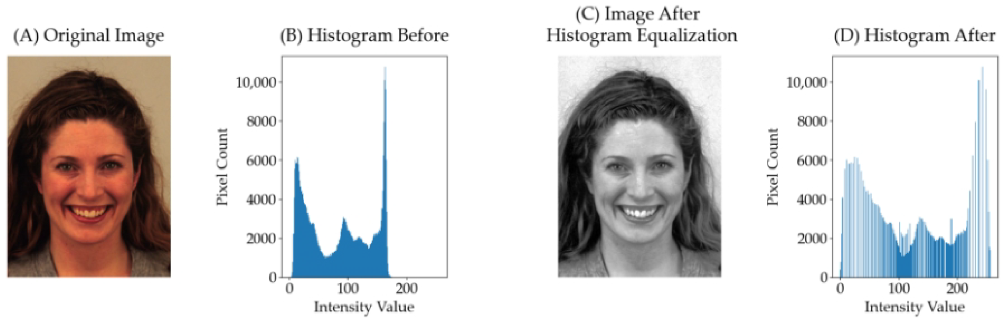
Figure 2 shows an image after histogram equalization. Figure 2A displays the original image from the KDEF dataset. Figure 2B depicts the corresponding histogram, illustrating the distribution of pixel intensities. Subsequently, Figure 2C exhibits the image post-histogram equalization, a process aimed at enhancing contrast and brightness. Finally, Figure 2D shows the resulting histogram, reflecting the altered intensity distribution after equalization. In Figure 2B,D, the X-axis denotes the intensity values, while the Y-axis represents the pixel counts.

Figure 2.
Histogram-equalized image from KDEF dataset.
3.2. Cosine Annealing
The cosine annealing strategy is a learning rate adjustment strategy used to dynamically adjust the learning rate in optimization algorithms. Its main idea is to simulate the annealing process of the cosine function, periodically changing the learning rate during the training process, so that the model can better make fine adjustments in the later stage of training and improve convergence performance. The original formula for the cosine annealing strategy is as follows:
Here, t in the numerator represents the total number of training cycles to the current stage, T in the denominator represents the set cosine annealing cycle, and represents the learning rate at a given point during the training process. Based on the ratio between t and T, the learning rate exhibits a cosine-like variation.
A characteristic of the cosine annealing strategy is that the learning rate will undergo periodic changes within the range of the maximum and minimum learning rates according to the annealing curve of the cosine function. This helps to make the model more stable in the later stages of training, avoiding oscillations or jumping out of local optima caused by an excessive learning rate, as well as situations where the learning rate is too small and the convergence speed is too slow [75].
3.3. Evaluation Matrices
Precision is the number of correctly predicted samples out of all predicted samples, which is a measure of classifier exactness. Recall is the number of correctly predicted samples out of the number of actual samples, which is a measure of classifier completeness. The F-measure is a harmonized mean of precision and recall, useful with uneven class distributions [76].
Here, true positive (TP) is when a positive sample is correctly classified as positive, and true negative (TN) is when a negative sample is correctly classified as negative. False negative (FN) is when a positive sample is classified as negative, and false positive (FP) is when a negative sample is classified as positive.
The AUC-ROC and AUC-PRC are performance metrics commonly used to evaluate the performances of binary classification models. The false positive rate (fpr) is calculated to determine these evaluation metrics. Here is the equation for the AUC-ROC:
Here, TPR (fpr) represents the true positive rate (TPR) at a given false positive rate (fpr), and d (fpr) represents the differential element for fpr. Here is the equation for the AIC-PRC:
Here, Precision (recall) represents the precision at a given recall value, and d (recall) represents the differential element for recall.
4. Implementation
In this section, we describe the datasets and the deep CNNs used in our work.
4.1. Datasets and Augmentation Techniques
- KDEF
The KDEF dataset comprises 4900 colored images depicting various human facial emotions. Additionally, the Averaged KDEF (AKDEF) dataset consists of averaged images derived from the original KDEF photos. Both the KDEF and AKDEF were built in 1998 and have since been made freely available to the academic community. Over the years, the KDEF has become widely utilized in research, with over 1500 publications using its data. The KDEF dataset encompasses seven distinct emotion classes: anger, neutral, disgust, fear, happy, sad, and surprise. Each image in the dataset is carefully labeled to denote the specific emotion portrayed by the individual. The images are in RGB format with a resolution of 224 × 224 pixels.
- CK+
The CK+ dataset [23] serves as a prominent benchmark dataset in the field of facial expression recognition research. It comprises a total of 981 images collected from 123 subjects, with each sequence depicting one of seven facial expressions: anger, contempt, disgust, fear, happy, sadness, and surprise. These expressions were elicited using the Facial Action Coding System (FACS), a standardized method for analyzing facial movements.
Each sequence within the CK+ dataset begins with a neutral expression, transitions to the target expression, and concludes with a return to the neutral expression. The images are captured under controlled laboratory conditions and are presented in a grayscale format, with a resolution of 640 by 490 pixels [77].
- The Filtered FER2013
The original FER2013 dataset comprises 35,887 grayscale images, each depicting cropped faces with dimensions of 48 × 48 pixels. These images are categorized into seven emotions: angry, disgust, fear, happy, neutral, sad, or surprise.
One notable aspect of the FER2013 dataset is its class imbalance, where the number of images varies significantly across emotion categories. Despite this, the dataset captures a diverse range of facial expressions encountered in real-life scenarios, including variations in lighting conditions, camera distance, and facial poses. The individuals depicted in the images represent diverse demographics, encompassing differences in age, race, and gender. Additionally, the dataset exhibits variations in the intensity of expressed emotions.
To address issues such as non-class-associated photos or non-face images, a filtered version of the FER2013 dataset was created by Bialek et al. [22]. This involved manual cleaning, removing images that did not correspond to any specific emotion category or were not depicting faces. Furthermore, instances of mislabeling were corrected, ensuring that images were assigned to the appropriate emotion group.
- Data Augmentation
We used various data augmentation techniques to enhance the diversity of the training dataset of the CK+ and KDEF and improve the generalization performances of the models. During the preprocessing phase, we applied augmentation methods such as rotation, horizontal shifting, and vertical shifting to the input images. Specifically, we configured the rotation_range parameter to allow random rotations within a range of −20 to +20 degrees. Additionally, we used width_shift_range and height_shift_range to introduce random horizontal and vertical shifts to the images, respectively, with a maximum displacement of 20% of the total width and height. Furthermore, we enabled horizontal flipping using the horizontal_flip parameter to further increase dataset variability. To ensure seamless augmentation, we used the ’nearest’ fill mode to interpolate pixel values for newly created pixels. Lastly, we applied pixel normalization by rescaling the pixel values of all images to a range between 0 and 1 using the rescale parameter, aiding in the convergence of the model during training.
For the FER2013 dataset, we employed different augmentation techniques compared to the KDEF and CK+ datasets. Specifically, we applied a rotation range of 10 degrees clockwise or counterclockwise, along with horizontal flipping. Additionally, we utilized a zoom range of [1.1, 1.2], allowing for random zooming between 1.1× and 1.2× the original size during training.
Regarding the data split, we adopted an 80% training, 10% validation, and 10% test split for both the CK+ and KDEF datasets. For the KDEF dataset specifically, we used three facial postures instead of the original five, resulting in 420 images per class, and this yielded 2940 images in total. For the filtered FER2013 dataset, we preserved the identical data split as described by Bialek et al. [22], comprising training (27,310), validation (3410), and test (3420) sets. Table 1 presents the counts of training, testing, and validation samples for the datasets used in our experiment. All experiments were conducted using subject-independent data across all datasets.

Table 1.
Data split for each dataset.
4.2. Experimental Setup
This work was conducted within a Docker environment, using the NVIDIA RTX 2080 GPU on a Windows 10 Education 64-bit system. The system was equipped with 32 GB of RAM and an Intel Core i7-9700k 3.60 GHz CPU. The transfer learning model was developed and executed using the Keras Python library (https://keras.io/api/ (accessed on 23 January 2024)). Visualizations of the results were generated using the matplotlib library (https://matplotlib.org/ (accessed on 23 January 2024)) and the seaborn library (https://seaborn.pydata.org/ (accessed on 23 January 2024)). Additionally, the SciKit-learn library (https://scikit-learn.org/stable/about.html (accessed on 23 January 2024)) was used to create evaluation matrices.
4.3. VGG Architectures
The task of FER was based on fine-tuned transfer learning from pre-trained VGG16 and VGG19 architectures. The VGG architecture, developed by Simonyan and Zisserman, achieved significant success as the runner-up in the ImageNet Large Scale Visual Recognition Competition (ILSVRC) in 2014. This architecture was chosen for several reasons: (i) demonstrable success on a variety of image classification tasks, (ii) native support provided by Keras, 5 which offers pre-trained models with publicly available weights, and (iii) a simpler implementation.
However, more complex models such as ResNet50 or DenseNet121 might face the problem of overfitting issues given a smaller dataset size. We employed VGG16 and VGG19, pre-trained on the ImageNet dataset, for classification purposes. In our approach, we unfroze the last four layers of VGG16 and the last five layers of VGG19, while freezing the remaining layers. This strategy allowed us to update the pre-trained ImageNet [78] weights with the weights learned from our specific datasets, enhancing the model’s ability to learn more effectively.
Following the basic VGG architecture, we added a global average pooling layer, a dropout layer, a dense layer with ReLU activation, another dropout layer, and, finally, a dense layer with softmax activation to classify the emotions. The proposed VGG16 and VGG19 model architectures are detailed in Table 2 and Table 3, respectively.
Table 2.
The proposed modified VGG16.
Table 3.
The proposed modified VGG19.
For comparison purposes, our experiment was structured in three distinct setups. Firstly, we maintained all layers of the base VGG19 and VGG16 models frozen, without applying any histogram equalization. Secondly, we fine-tuned the VGG19 and VGG16 architectures by unfreezing the last four layers of VGG16 and the last five layers of VGG19, while keeping the remaining layers frozen. This setup also did not include any histogram equalization. Lastly, we incorporated histogram equalization into the final experimental setup, along with fine-tuning the models as described in the second setup. For the KDEF dataset, our initial step involved optimizing the data for histogram equalization by converting the images to grayscale. Subsequently, to obtain the RGB format suitable for a pre-trained VGG network, we further transformed the grayscale images into RGB format. During this process, each pixel in the grayscale image replicated its intensity value across all three color channels. A general overview of our framework can be found in Figure 1.
4.4. Hyperparameters
For training our models on different datasets, we used various hyperparameters to optimize the performance. These hyperparameters included the Input Size, Batch Size, Epochs, Learning Rate, Early Stopping, Learning Rate Scheduler, Dropout Rate, and L2 Regularization. The specifics of these parameters for different datasets are outlined in Table 4.
Table 4.
Hyperparameters for the models on different datasets.
In the CK+ dataset, the original images were re-sized to (224, 224, 3). We applied a dropout rate of 0.5 for regularization purposes. Additionally, we implemented early stopping, which halts the training process if the validation accuracy does not improve for five consecutive epochs to prevent overfitting.
We used the same techniques for data augmentation and resizing on the KDEF dataset. We also used early stopping and a learning rate scheduler. If the validation accuracy did not improve for three consecutive epochs, the learning rate was multiplied by 0.5 to decrease it. If the accuracy did not increase for five consecutive epochs, the training process was stopped. The dropout rate for this dataset was set to 0.1, and l2 kernel regularization with a value of 0.01 was applied for optimal performance.
For the FER2013 dataset, we conducted extensive experimentation with various learning strategies and optimizers. Through our analysis, we discovered that employing cosine annealing with the adam optimizer yielded the most accurate results. During training, initial_lr set the starting learning rate, while T_maxdefined the duration of a cycle of the cosine annealing schedule. The learning rate decreased gradually from the initial value to a minimum over T_max epochs, following a cosine curve pattern. Additionally, we explored different image sizes and were surprised to find that the transfer learning models performed exceptionally well when the images were resized to (144,144,3). In terms of batch size, we used the value of 64, which differed from the batch sizes used in the other datasets. Furthermore, we also found that the optimal dropout rate and l2 regularization penalty were 0.1 for this dataset. Regarding model training strategies, we initially employed a similar approach to that used in the CK+ dataset, wherein the model training would stop if the validation accuracy did not improve for five consecutive epochs. Subsequently, we saved the models and proceeded to train them again using cosine annealing for an additional 30 epochs. The initial learning rate was set to 0.0001, and then it gradually decreased according to the equation specified in Equation (3). Afterward, the model was trained using this gradually decreasing learning rate.
5. Results
5.1. KDEF
For the KDEF dataset, specifically, the hyper-tuned VGG19 model with histogram equalization achieved a commendable accuracy of 95.92%, while the fine-tuned VGG19 model without histogram equalization lagged by just 1.7% (Table 5). Similar trends were also observed for the VGG16 architectures, where histogram equalization helped the fine-tuned models achieve slightly better results. On the other hand, the models with all layers frozen and without histogram equalization, demonstrated inferior performances.
Table 5.
Performance comparison of different models on various datasets.
However, the most significant results are highlighted in Table 6, which presents class-wise evaluation metrics for our best model, the fine-tuned VGG19 model with histogram equalization. Notably, the highest scores were observed in the happy class, with the precision, recall, and F1-score all reaching 100%.
Table 6.
Performance of fine-tuned VGG19 on different classes on the KDEF dataset.
5.2. CK+
For the CK+ dataset, our models achieved the highest accuracies among the various architectures. Specifically, the fine-tuned VGG16 and VGG19 models, both with and without histogram equalization, demonstrated exceptional performances with accuracies of 100% and 98.99%, respectively (Table 5). Additionally, these models exhibited strong performances in terms of weighted F1, AUC-ROC, and AUC-PRC metrics. The VGG16 and VGG19 models, in which the layers of the base models were frozen and not fine-tuned, exhibited lower performances across all evaluation metrics, achieving 96.97% and 90.91%, respectively.
To gain insights into the inner workings of our CNN models, we employed Grad-CAM (Gradient-weighted Class Activation Mapping) [79]. Grad-CAM is a visualization technique that highlights important regions of an input image used by a CNN for classification. By examining the Grad-CAM visualizations (Figure 3), we observed that our models were effectively focusing on crucial areas (red marked areas) where important features are located. This suggests that our models are making informed decisions based on relevant image features.
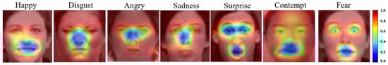
Figure 3.
GradCam from CK+ Dataset.
Furthermore, the superiority of our models can be visualized when we examine its confusion matrix. Its confusion matrix (Figure 4) reveals a zero misclassification rate on the CK+ datasets.
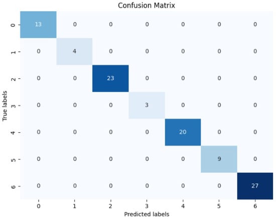
Figure 4.
Confusion matrix for fine-tuned VGG16 model with histogram equalization on CK+ dataset.
5.3. Filtered FER2013
In the case of the Filtered FER2013 dataset, the VGG16 model with histogram equalization outperformed the other models, achieving an accuracy of almost 69.65%. The performance difference was marginal for the fine-tuned VGG19 models with and without histogram equalization, achieving accuracies of 69.44% and 60.06%, respectively.
The effectiveness of the models is further highlighted in Table 7, where the per-class accuracy demonstrates how well the model performs across different classes with the FER2013 dataset.
Table 7.
Performance of fine-tuned VGG16 model with histogram equalization on different classes in the FER2013 dataset.
5.4. Comparison of Methods
The comparison of methods primarily focused on the accuracy metric, as most other researchers did not employ additional metrics like the AUC-ROC or AUC-PRC. The comparison of methods based on the KDEF, CK+, and FER2013 is depicted in Table 8, Table 9 and Table 10.
Table 8.
Comparison of methods on KDEF dataset.
Table 9.
Comparison of methods on CK+ dataset.
Table 10.
Comparison of methods on FER2013 dataset.
Our model demonstrated an exceptional performance on the KDEF dataset compared to state-of-the-art works. The closest contender was the model in the study by Sahoo et al., achieving an accuracy of nearly 93% using a transfer learning model based on VGG19. On the CK+ dataset, our model also showcases supremacy. Although the work of Dar et al. achieved the same accuracy, their model was notably complex, with each convolutional block comprising approximately 18 layers.
However, the discussion primarily centers around the FER2013 dataset, where our model exhibited a relatively good performance. We utilized the filtered FER2013 dataset from the work of Bialek et al., where their single five-layer model achieved an accuracy of approximately 70.09%. Despite attempting to implement the same model on the filtered FER2013 dataset, we achieved only a 68.27% accuracy. Therefore, we implemented our own pipeline, achieving an accuracy of almost 69.65%. Moreover, despite employing a simpler model based on pre-trained VGG16, our model compares favorably with other works that utilize more complex architectures. Notably, our model takes less time because of the lower number of parameters that it is using.
6. Discussion
This section of our paper highlights key notations and compares our models with existing works in the field. We delve into specific notations crucial for understanding our approach and provide a thorough comparison of our models with those previously established in the literature.
The comparison between models with all layers frozen with no histogram and those with fine-tuned models with no histogram reveals significant differences in the performances across datasets. For instance, on the KDEF dataset, the VGG19 with all layers frozen and no histogram achieved an accuracy of 54.76%, whereas the fine-tuned VGG19 with no Histogram achieved nearly 94.22%. This variation underscores the limitations of freezing all layers, as it limits the model’s adaptability to the new task/domain by preserving fixed feature extraction mechanisms. Oppositely, unfreezing the last five layers allows for fine-tuning, enabling the model to learn task-specific representations and enhance the performance using pre-trained weights while accommodating adjustments to suit the new task requirements.
Furthermore, we proceed to compare the models’ performance post-histogram equalization. Notably, all hyper-tuned models exhibited slightly improved performances with histogram equalization. As indicated in Table 5, hyper-tuned models using histogram-equalized images showed a 0.3–2% enhancement on average compared to their counterparts without histogram equalization. However, exceptions were observed on the CK+ dataset, where both hyper-tuned models, with and without histogram equalization, exhibited similar performances.
In the case of the Filtered FER2013 dataset, one interesting observation worth discussing is the performance on the FER2013 dataset with the image size set to 144 × 144. Despite the original VGG16 and VGG19 models being trained on the 224 × 224 × 3 ImageNet dataset, the 144 × 144 image size showed promising results across all experiments. This deviation from the conventional image size might be attributed to the potential loss of information and degradation of image quality when resizing an image to larger dimensions. When resizing an image to a larger size, the existing pixels are stretched to fill the new dimensions, which can lead to blurriness or pixelation. This loss of information may have been mitigated by selecting an optimum size of 144 × 144, which preserved the originality of the image while maintaining a balance between image quality and resolution.
Moreover, when we applied cosine annealing to the fine-tuned VGG16 models with histograms, the model’s accuracy initially plateaued at around 67.57% on the FER2013 dataset. However, after reloading the model and running the model for an additional 30 epochs with cosine annealing, the accuracy improved to 69.65%. But which specific features of the cosine annealing rate differ from those in normal learning cycles, resulting in enhancements in model performance should be interesting to find. Normal training cycles involve updating model parameters over multiple epochs to minimize loss and improve performance, focusing on data-driven optimization. In contrast, cosine annealing cycles specifically regulate the learning rate schedule within each training cycle, dynamically adjusting it over epochs according to a cosine curve pattern. While normal training cycles primarily target parameter updates, cosine annealing cycles aim to optimize the learning rate schedule, potentially enhancing training efficiency and model performance. This adaptive learning rate scheduling of cosine annealing allowed the model to escape local minima and explore the parameter space more effectively, ultimately leading to an improved performance.
When handling a small dataset like CK+, training models like VGG16 and VGG19 can be prone to overfitting due to their extensive parameter count. However, employing regularization techniques and training techniques, coupled with data augmentation, aids in effectively training the model with this limited data. This effectiveness can be seen in Figure 3, where the model effectively identifies crucial features in facial data across various classes, showcasing its robustness even with limited data.
7. Conclusions
This paper presents a thorough comparative analysis of FER methods using CNN architectures through extensive experiments and prediction metrics such as the AUC-ROC, AUC-PRC, and F1 scores for each model. Comparing these methodologies offers a nuanced exploration of their strengths and limitations, shedding light on areas for improvement and potential avenues for further research. This paper demonstrates that the application of histogram equalization along with data augmentation can improve accuracy in recognizing facial emotions. Another significant contribution of this paper is in optimizing the performance of pre-trained simple architectures like VGG across various dataset sizes by employing different regularization techniques, callbacks, and learning scheduler techniques on selected datasets. Instead of opting for complex models, this study demonstrates that careful fine-tuning can lead to a better classification accuracy with simpler architectures.
The primary limitation of our study lies in the simplistic architecture used. Compared to the methodologies employed by most studies outlined in Table 10, our approach is notably less complex. Additionally, for the FER2013 dataset, the potential incorporation of auxiliary data could enhance model performance. Currently, facial landmark recognition and attention mechanisms are used widely for facial recognition problems. Integrating these techniques could prove beneficial for improving the performances of our models in future endeavors.
Author Contributions
The conceptualization and methodology were developed by J.H.C., Q.L. and S.R. J.H.C. handled data curation, software development, and validation, as well as taking the lead in preparing the original draft for writing. Q.L. and S.R. conducted the review and editing of the writing, and they also provided supervision throughout the experiment. Funding for the resources used in the experiment was provided by S.R. All authors have read and agreed to the published version of the manuscript.
Funding
This research was funded by Natural Sciences and Engineering Research Council Discovery Grant #194376.
Data Availability Statement
The research presented in this article was performed using the publicly available image datasets KDEF [21], CK+ [23], and the version of FER2013 that was derived from the paper ‘Efficient Approach to Face Emotion Recognition with Convolutional Neural Networks’ [22].
Conflicts of Interest
The manuscript is approved for publication by all authors. The work described is original research that has not been published previously and is not under consideration for publication elsewhere.
References
- Ekman, P. Cross-cultural studies of facial expression. Darwin Facial Expr. Century Res. Rev. 1973, 169222, 45–60. [Google Scholar]
- Ramsay, R.W. Speech patterns and personality. Lang. Speech 1968, 11, 54–63. [Google Scholar] [CrossRef] [PubMed]
- Fast, J. Body Language; Simon and Schuster: New York, NY, USA, 1970; Volume 82348. [Google Scholar]
- Newmark, C. Charles Darwin: The expression of the emotions in man and animals. In Schlüsselwerke der Emotionssoziologie; Springer: Berlin/Heidelberg, Germany, 2022; pp. 111–115. [Google Scholar]
- Ragsdale, J.W.; Van Deusen, R.; Rubio, D.; Spagnoletti, C. Recognizing patients’ emotions: Teaching health care providers to interpret facial expressions. Acad. Med. 2016, 91, 1270–1275. [Google Scholar] [CrossRef] [PubMed]
- Suhaimi, N.S.; Mountstephens, J.; Teo, J. EEG-Based Emotion Recognition: A State-of-the-Art Review of Current Trends and Opportunities. Comput. Intell. Neurosci. 2020, 2020, 8875426. [Google Scholar] [CrossRef] [PubMed]
- Fernández-Caballero, A.; Martínez-Rodrigo, A.; Pastor, J.M.; Castillo, J.C.; Lozano-Monasor, E.; López, M.T.; Zangróniz, R.; Latorre, J.M.; Fernández-Sotos, A. Smart environment architecture for emotion detection and regulation. J. Biomed. Inform. 2016, 64, 55–73. [Google Scholar] [CrossRef] [PubMed]
- Mattavelli, G.; Pisoni, A.; Casarotti, A.; Comi, A.; Sera, G.; Riva, M.; Bizzi, A.; Rossi, M.; Bello, L.; Papagno, C. Consequences of brain tumour resection on emotion recognition. J. Neuropsychol. 2019, 13, 1–21. [Google Scholar] [CrossRef] [PubMed]
- Suchitra; Suja, P.; Tripathi, S. Real-time emotion recognition from facial images using Raspberry Pi II. In Proceedings of the 2016 3rd International Conference on Signal Processing and Integrated Networks (SPIN), Noida, India, 11–12 February 2016; IEEE: Piscataway, NJ, USA, 2016; pp. 666–670. [Google Scholar]
- Ojala, T.; Pietikäinen, M.; Harwood, D. A comparative study of texture measures with classification based on featured distributions. Pattern Recognit. 1996, 29, 51–59. [Google Scholar] [CrossRef]
- Jolliffe, I.T.; Cadima, J. Principal component analysis: A review and recent developments. Philos. Trans. R. Soc. A Math. Phys. Eng. Sci. 2016, 374, 20150202. [Google Scholar] [CrossRef]
- Van der Maaten, L.; Hinton, G. Visualizing data using t-SNE. J. Mach. Learn. Res. 2008, 9, 2579–2605. [Google Scholar]
- Cortes, C.; Vapnik, V. Support-vector networks. Mach. Learn. 1995, 20, 273–297. [Google Scholar] [CrossRef]
- Breiman, L. Random forests. Mach. Learn. 2001, 45, 5–32. [Google Scholar] [CrossRef]
- Payal, P.; Goyani, M.M. A comprehensive study on face recognition: Methods and challenges. Imaging Sci. J. 2020, 68, 114–127. [Google Scholar] [CrossRef]
- O’shea, K.; Nash, R. An introduction to convolutional neural networks. arXiv 2015, arXiv:1511.08458. [Google Scholar]
- Hochreiter, S. The vanishing gradient problem during learning recurrent neural nets and problem solutions. Int. J. Uncertainty, Fuzziness Knowl.-Based Syst. 1998, 6, 107–116. [Google Scholar] [CrossRef]
- Simonyan, K.; Zisserman, A. Very deep convolutional networks for large-scale image recognition. arXiv 2014, arXiv:1409.1556. [Google Scholar]
- He, K.; Zhang, X.; Ren, S.; Sun, J. Deep Residual Learning for Image Recognition. arXiv 2015, arXiv:1512.03385. [Google Scholar]
- Huang, G.; Liu, Z.; van der Maaten, L.; Weinberger, K.Q. Densely Connected Convolutional Networks. arXiv 2018, arXiv:1608.06993. [Google Scholar]
- Lundqvist, D.; Flykt, A.; Öhman, A. Karolinska directed emotional faces. PsycTESTS Dataset 1998, 91, 630. [Google Scholar]
- Białek, C.; Matiolański, A.; Grega, M. An Efficient Approach to Face Emotion Recognition with Convolutional Neural Networks. Electronics 2023, 12, 2707. [Google Scholar] [CrossRef]
- Lucey, P.; Cohn, J.F.; Kanade, T.; Saragih, J.; Ambadar, Z.; Matthews, I. The extended cohn-kanade dataset (ck+): A complete dataset for action unit and emotion-specified expression. In Proceedings of the 2010 Ieee Computer Society Conference on Computer Vision and Pattern Recognition-Workshops, San Francisco, CA, USA, 13–18 June 2010; IEEE: Piscataway, NJ, USA, 2010; pp. 94–101. [Google Scholar]
- Xie, Y.; Ning, L.; Wang, M.; Li, C. Image Enhancement Based on Histogram Equalization. J. Phys. Conf. Ser. 2019, 1314, 012161. [Google Scholar] [CrossRef]
- Gotmare, A.; Keskar, N.S.; Xiong, C.; Socher, R. A closer look at deep learning heuristics: Learning rate restarts, warmup and distillation. arXiv 2018, arXiv:1810.13243. [Google Scholar]
- Hanley, J.A.; McNeil, B.J. The meaning and use of the area under a receiver operating characteristic (ROC) curve. Radiology 1982, 143, 29–36. [Google Scholar] [CrossRef] [PubMed]
- Powers, D.M. Evaluation: From precision, recall and F-measure to ROC, informedness, markedness and correlation. arXiv 2020, arXiv:2010.16061. [Google Scholar]
- Xiao-Xu, Q.; Wei, J. Application of wavelet energy feature in facial expression recognition. In Proceedings of the 2007 International Workshop on Anti-Counterfeiting, Security and Identification (ASID), Xizmen, China, 16–18 April 2007; IEEE: Piscataway, NJ, USA, 2007; pp. 169–174. [Google Scholar]
- Lyons, M.; Kamachi, M.; Gyoba, J. The Japanese Female Facial Expression (JAFFE) Dataset. 1998. Available online: https://zenodo.org/records/3451524 (accessed on 1 May 2024).
- Tyagi, M. Hog (Histogram of Oriented Gradients): An Overview; Towards Data Science: Toronto, ON, Canada, 2021; Volume 4. [Google Scholar]
- Ahonen, T.; Rahtu, E.; Ojansivu, V.; Heikkila, J. Recognition of blurred faces using local phase quantization. In Proceedings of the 2008 19th International Conference on Pattern Recognition, Tampa, FL, USA, 8–11 December 2008; IEEE: Piscataway, NJ, USA, 2008; pp. 1–4. [Google Scholar]
- Lloyd, S. Least squares quantization in PCM. IEEE Trans. Inf. Theory 1982, 28, 129–137. [Google Scholar] [CrossRef]
- Lee, H.; Kim, S. SSPNet: Learning spatiotemporal saliency prediction networks for visual tracking. Inf. Sci. 2021, 575, 399–416. [Google Scholar] [CrossRef]
- Yang, S.; Bhanu, B. Facial expression recognition using emotion avatar image. In Proceedings of the 2011 IEEE International Conference on Automatic Face & Gesture Recognition (FG), Santa Barbara, CA, USA, 21–25 March 2011; IEEE: Piscataway, NJ, USA, 2011; pp. 866–871. [Google Scholar]
- Dhall, A.; Asthana, A.; Goecke, R.; Gedeon, T. Emotion recognition using PHOG and LPQ features. In Proceedings of the 2011 IEEE International Conference on Automatic Face & Gesture Recognition (FG), Santa Barbara, CA, USA, 21–25 March 2011; IEEE: Piscataway, NJ, USA, 2011; pp. 878–883. [Google Scholar]
- Cootes, T.F.; Edwards, G.J.; Taylor, C.J. Active appearance models. In Proceedings of the Computer Vision—ECCV’98: 5th European Conference on Computer Vision, Freiburg, Germany, 2–6 June 1998; Springer: Berlin/Heidelberg, Germany, 1998; Volume II 5, pp. 484–498. [Google Scholar]
- Sharmin, N.; Brad, R. Optimal filter estimation for Lucas-Kanade optical flow. Sensors 2012, 12, 12694–12709. [Google Scholar] [CrossRef]
- Pu, X.; Fan, K.; Chen, X.; Ji, L.; Zhou, Z. Facial expression recognition from image sequences using twofold random forest classifier. Neurocomputing 2015, 168, 1173–1180. [Google Scholar] [CrossRef]
- Golzadeh, H.; Faria, D.R.; Manso, L.J.; Ekárt, A.; Buckingham, C.D. Emotion recognition using spatiotemporal features from facial expression landmarks. In Proceedings of the 2018 International Conference on Intelligent Systems (IS), Funchal, Portugal, 25–27 September 2018; IEEE: Piscataway, NJ, USA, 2018; pp. 789–794. [Google Scholar]
- Aifanti, N.; Papachristou, C.; Delopoulos, A. The MUG facial expression database. In Proceedings of the 11th International Workshop on Image Analysis for Multimedia Interactive Services WIAMIS 10, Desenzano del Garda, Italy, 12–14 April 2010; IEEE: Piscataway, NJ, USA, 2010; pp. 1–4. [Google Scholar]
- Viola, P.; Jones, M. Rapid object detection using a boosted cascade of simple features. In Proceedings of the 2001 IEEE Computer Society Conference on Computer Vision and Pattern Recognition, CVPR 2001, Kauai, HI, USA, 8–14 December 2001; Volume 1, p. I. [Google Scholar] [CrossRef]
- Freeman, W.T.; Roth, M. Orientation histograms for hand gesture recognition. In Proceedings of the International Workshop on Automatic Face and Gesture Recognition, Zurich, Switzerland, 26–28 June 1995; Citeseer: Princeton, NJ, USA, 1995; Volume 12, pp. 296–301. [Google Scholar]
- Liew, C.F.; Yairi, T. Facial expression recognition and analysis: A comparison study of feature descriptors. IPSJ Trans. Comput. Vis. Appl. 2015, 7, 104–120. [Google Scholar] [CrossRef]
- Chen, T.; Guestrin, C. Xgboost: A scalable tree boosting system. In Proceedings of the 22nd Acm Sigkdd International Conference on Knowledge Discovery and Data Mining, San Francisco, CA, USA, 13–17 August 2016; pp. 785–794. [Google Scholar]
- Thakare, C.; Chaurasia, N.K.; Rathod, D.; Joshi, G.; Gudadhe, S. Comparative analysis of emotion recognition system. Int. Res. J. Eng. Technol. 2019, 6, 380–384. [Google Scholar]
- Goodfellow, I.J.; Erhan, D.; Carrier, P.L.; Courville, A.; Mirza, M.; Hamner, B.; Cukierski, W.; Tang, Y.; Thaler, D.; Lee, D.H.; et al. Challenges in representation learning: A report on three machine learning contests. In Proceedings of the Neural Information Processing: 20th International Conference, ICONIP 2013, Daegu, Republic of Korea, 3–7 November 2013; Part III 20. Springer: Berlin/Heidelberg, Germany, 2013; pp. 117–124. [Google Scholar]
- Jalal, A.; Tariq, U. The LFW-gender dataset. In Proceedings of the Computer Vision–ACCV 2016 Workshops: ACCV 2016 International Workshops, Taipei, Taiwan, 20–24 November 2016; Revised Selected Papers, Part III 13. Springer: Berlin/Heidelberg, Germany, 2017; pp. 531–540. [Google Scholar]
- Zhang, W.; He, X.; Lu, W. Exploring discriminative representations for image emotion recognition with CNNs. IEEE Trans. Multimed. 2019, 22, 515–523. [Google Scholar] [CrossRef]
- Howard, A.G.; Zhu, M.; Chen, B.; Kalenichenko, D.; Wang, W.; Weyand, T.; Andreetto, M.; Adam, H. Mobilenets: Efficient convolutional neural networks for mobile vision applications. arXiv 2017, arXiv:1704.04861. [Google Scholar]
- Badrulhisham, N.A.S.; Mangshor, N.N.A. Emotion Recognition Using Convolutional Neural Network (CNN). J. Phys. Conf. Ser. 2021, 1962, 012040. [Google Scholar] [CrossRef]
- Chandrasekaran, G.; Antoanela, N.; Andrei, G.; Monica, C.; Hemanth, J. Visual sentiment analysis using deep learning models with social media data. Appl. Sci. 2022, 12, 1030. [Google Scholar] [CrossRef]
- Szegedy, C.; Ioffe, S.; Vanhoucke, V.; Alemi, A.A. Inception-v4, inception-ResNet and the impact of residual connections on learning. In Proceedings of the Thirty-First AAAI Conference on Artificial Intelligence, San Francisco, CA, USA, 4–9 February 2017; AAAI Press: Washington, DC, USA, 2017. AAAI’17. pp. 4278–4284. [Google Scholar]
- Zagoruyko, S.; Komodakis, N. Wide residual networks. arXiv 2016, arXiv:1605.07146. [Google Scholar]
- Subudhiray, S.; Palo, H.K.; Das, N. Effective recognition of facial emotions using dual transfer learned feature vectors and support vector machine. Int. J. Inf. Technol. 2023, 15, 301–313. [Google Scholar] [CrossRef]
- Sandler, M.; Howard, A.; Zhu, M.; Zhmoginov, A.; Chen, L.C. Mobilenetv2: Inverted residuals and linear bottlenecks. In Proceedings of the IEEE Conference on Computer Vision and Pattern Recognition, Salt Lake City, UT, USA, 18–23 June 2018; pp. 4510–4520. [Google Scholar]
- Kaur, S.; Kulkarni, N. FERFM: An Enhanced Facial Emotion Recognition System Using Fine-tuned MobileNetV2 Architecture. IETE J. Res. 2023, 1–15. [Google Scholar] [CrossRef]
- Mollahosseini, A.; Hasani, B.; Mahoor, M.H. Affectnet: A database for facial expression, valence, and arousal computing in the wild. IEEE Trans. Affect. Comput. 2017, 10, 18–31. [Google Scholar] [CrossRef]
- Szegedy, C.; Liu, W.; Jia, Y.; Sermanet, P.; Reed, S.; Anguelov, D.; Erhan, D.; Vanhoucke, V.; Rabinovich, A. Going deeper with convolutions. In Proceedings of the IEEE Conference on Computer Vision and Pattern Recognition, Boston, MA, USA, 7–12 June 2015; pp. 1–9. [Google Scholar]
- He, K.; Zhang, X.; Ren, S.; Sun, J. Deep residual learning for image recognition. In Proceedings of the IEEE Conference on Computer Vision and Pattern Recognition, Las Vegas, NV, USA, 27–30 June 2016; pp. 770–778. [Google Scholar]
- Zavarez, M.V.; Berriel, R.F.; Oliveira-Santos, T. Cross-Database Facial Expression Recognition Based on Fine-Tuned Deep Convolutional Network. In Proceedings of the 2017 30th SIBGRAPI Conference on Graphics, Patterns and Images (SIBGRAPI), Niteroi, Brazil, 17–20 October 2017; pp. 405–412. [Google Scholar] [CrossRef]
- Puthanidam, R.V.; Moh, T.S. A hybrid approach for facial expression recognition. In Proceedings of the 12th International Conference on Ubiquitous Information Management and Communication, Langkawi, Malaysia, 5–7 January 2018; pp. 1–8. [Google Scholar]
- Chen, Y.; Liu, Z.; Wang, X.; Xue, S.; Yu, J.; Ju, Z. Combating Label Ambiguity with Smooth Learning for Facial Expression Recognition. In Proceedings of the International Conference on Intelligent Robotics and Applications, Hangzhou, China, 5–7 July 2023; Springer: Berlin/Heidelberg, Germany, 2023; pp. 127–136. [Google Scholar]
- Liu, X.; Vijaya Kumar, B.; You, J.; Jia, P. Adaptive deep metric learning for identity-aware facial expression recognition. In Proceedings of the IEEE Conference on Computer Vision and Pattern Recognition Workshops, Honolulu, HI, USA, 21–26 July 2017; pp. 20–29. [Google Scholar]
- Pantic, M.; Valstar, M.; Rademaker, R.; Maat, L. Web-based database for facial expression analysis. In Proceedings of the 2005 IEEE International Conference on Multimedia and Expo, Amsterdam, The Netherlands, 6–9 July 2005; IEEE: Piscataway, NJ, USA, 2005; p. 5. [Google Scholar]
- Dar, T.; Javed, A.; Bourouis, S.; Hussein, H.S.; Alshazly, H. Efficient-SwishNet based system for facial emotion recognition. IEEE Access 2022, 10, 71311–71328. [Google Scholar] [CrossRef]
- Zahara, L.; Musa, P.; Wibowo, E.P.; Karim, I.; Musa, S.B. The facial emotion recognition (FER-2013) dataset for prediction system of micro-expressions face using the convolutional neural network (CNN) algorithm based Raspberry Pi. In Proceedings of the 2020 Fifth International Conference on Informatics and Computing (ICIC), Gorontalo, Indonesia, 3–4 November 2020; IEEE: Piscataway, NJ, USA, 2020; pp. 1–9. [Google Scholar]
- Minaee, S.; Minaei, M.; Abdolrashidi, A. Deep-emotion: Facial expression recognition using attentional convolutional network. Sensors 2021, 21, 3046. [Google Scholar] [CrossRef] [PubMed]
- Fei, Z.; Yang, E.; Yu, L.; Li, X.; Zhou, H.; Zhou, W. A novel deep neural network-based emotion analysis system for automatic detection of mild cognitive impairment in the elderly. Neurocomputing 2022, 468, 306–316. [Google Scholar] [CrossRef]
- Krizhevsky, A.; Sutskever, I.; Hinton, G.E. ImageNet classification with deep convolutional neural networks. Commun. ACM 2017, 60, 84–90. [Google Scholar] [CrossRef]
- Iandola, F.N.; Han, S.; Moskewicz, M.W.; Ashraf, K.; Dally, W.J.; Keutzer, K. SqueezeNet: AlexNet-level accuracy with 50x fewer parameters and <0.5 MB model size. arXiv 2016, arXiv:1602.07360. [Google Scholar]
- Dhall, A.; Goecke, R.; Lucey, S.; Gedeon, T. Static facial expression analysis in tough conditions: Data, evaluation protocol and benchmark. In Proceedings of the 2011 IEEE International Conference on Computer Vision Workshops (ICCV Workshops), Barcelona, Spain, 6–13 November 2011; IEEE: Piscataway, NJ, USA, 2011; pp. 2106–2112. [Google Scholar]
- Sahoo, G.K.; Das, S.K.; Singh, P. Performance Comparison of Facial Emotion Recognition: A Transfer Learning-Based Driver Assistance Framework for In-Vehicle Applications. Circuits Syst. Signal Process. 2023, 42, 4292–4319. [Google Scholar] [CrossRef]
- Mahesh, V.G.; Chen, C.; Rajangam, V.; Raj, A.N.J.; Krishnan, P.T. Shape and texture aware facial expression recognition using spatial pyramid Zernike moments and law’s textures feature set. IEEE Access 2021, 9, 52509–52522. [Google Scholar] [CrossRef]
- Gonzalez, R.C.; Woods, R.E. Digital Image Processing, 3rd ed.; Prentice-Hall, Inc.: Saddle River, NJ, USA, 2006. [Google Scholar]
- Zhang, C.; Shao, Y.; Sun, H.; Xing, L.; Zhao, Q.; Zhang, L. The WuC-Adam algorithm based on joint improvement of Warmup and cosine annealing algorithms. Math. Biosci. Eng. 2024, 21, 1270–1285. [Google Scholar] [CrossRef] [PubMed]
- Hall, M.; Frank, E.; Holmes, G.; Pfahringer, B.; Reutemann, P.; Witten, I.H. The WEKA data mining software: An update. ACM SIGKDD Explor. Newsl. 2009, 11, 10–18. [Google Scholar] [CrossRef]
- Barhoumi, C.; Ayed, Y.B. Unlocking the Potential of Deep Learning and Filter Gabor for Facial Emotion Recognition. In Proceedings of the International Conference on Computational Collective Intelligence, Budapest, Hungary, 27–29 September 2023; Springer: Berlin/Heidelberg, Germany, 2023; pp. 97–110. [Google Scholar]
- Deng, J.; Dong, W.; Socher, R.; Li, L.J.; Li, K.; Fei-Fei, L. ImageNet: A large-scale hierarchical image database. In Proceedings of the 2009 IEEE Conference on Computer Vision and Pattern Recognition, Miami, FL, USA, 20–25 June 2009; pp. 248–255. [Google Scholar] [CrossRef]
- Selvaraju, R.R.; Cogswell, M.; Das, A.; Vedantam, R.; Parikh, D.; Batra, D. Grad-CAM: Visual Explanations from Deep Networks via Gradient-Based Localization. Int. J. Comput. Vis. 2019, 128, 336–359. [Google Scholar] [CrossRef]


Disclaimer/Publisher’s Note: The statements, opinions and data contained in all publications are solely those of the individual author(s) and contributor(s) and not of MDPI and/or the editor(s). MDPI and/or the editor(s) disclaim responsibility for any injury to people or property resulting from any ideas, methods, instructions or products referred to in the content. |
© 2024 by the authors. Licensee MDPI, Basel, Switzerland. This article is an open access article distributed under the terms and conditions of the Creative Commons Attribution (CC BY) license (https://creativecommons.org/licenses/by/4.0/).