Semi-Self-Supervised Domain Adaptation: Developing Deep Learning Models with Limited Annotated Data for Wheat Head Segmentation

Abstract

Precision agriculture involves the application of advanced technologies to improve agricultural productivity, efficiency, and profitability while minimizing waste and environmental impacts. Deep learning approaches enable automated decision-making for many visual tasks. However, in the agricultural domain, variability in growth stages and environmental conditions, such as weather and lighting, presents significant challenges to developing deep-learning-based techniques that generalize across different conditions. The resource-intensive nature of creating extensive annotated datasets that capture these variabilities further hinders the widespread adoption of these approaches. To tackle these issues, we introduce a semi-self-supervised domain adaptation technique based on deep convolutional neural networks with a probabilistic diffusion process, requiring minimal manual data annotation. Using only three manually annotated images and a selection of video clips from wheat fields, we generated a large-scale computationally annotated dataset of image–mask pairs and a large dataset of unannotated images extracted from video frames. We developed a two-branch convolutional encoder–decoder model architecture that uses both synthesized image–mask pairs and unannotated images, enabling effective adaptation to real images. The proposed model achieved a Dice score of 80.7% on an internal test dataset and a Dice score of 64.8% on an external test set composed of images from five countries and spanning 18 domains, indicating its potential to develop generalizable solutions that could encourage the wider adoption of advanced technologies in agriculture.

1. Introduction

Precision agriculture refers to the use of advanced technologies, including GPS guidance, control systems, sensors, robotics, drones, autonomous vehicles, and variable rate technology, to optimize farm management. It aims to reduce costs and increase yields in farming while ensuring sustainability and environmental protection [1]. Deep learning (DL) methodologies can offer efficient, automated, and data-driven decision-making in agricultural practices. DL has demonstrated significant advancements in visual data analysis across various tasks, including image classification [2,3], object detection [4,5], semantic segmentation [6,7,8], and instance segmentation [9,10,11]. Automated visual monitoring of agricultural fields can aid in the early identification of issues such as pest infestations, diseases, and nutrient deficiencies while optimizing resource utilization. Consequently, this approach facilitates timely interventions, which can lead to enhanced crop yields, improved quality of harvests, and increased overall operational efficiency, thereby ensuring sustainability.

However, the wide adoption of DL approaches for crop monitoring faces significant challenges. Agricultural fields are constantly changing environments. For example, a crop field in the early growth stages is substantially different from the same field in the later stages of growth. Additionally, these systems must operate accurately under various weather and lighting conditions. This challenges the generalizability of DL models because models trained on data from a specific growth stage of a field might not generalize well to the same crop at different growth stages. In the DL context, this phenomenon is known as a distribution shift [12,13]. One could develop a large-scale dataset encompassing various crop growth stages and environmental conditions to alleviate this issue. However, this approach presents challenges to data collection and annotation. Collecting data from various growth stages of crop fields under various weather and lighting conditions is time-consuming. Further, annotating agricultural images is particularly challenging, often requiring pixel-level annotation. These images frequently contain numerous objects of interest—e.g., wheat spikes in a wheat field—making the data annotation process laborious.

Environmental conditions—such as climate, soil quality, geographical location, and pest and disease pressure—significantly contribute to data variation in crop datasets. Variations in temperature, precipitation, humidity, soil types, regional microclimates, and pest and disease prevalence collectively influence crop growth and yield outcomes. Further, phenotypic varieties introduce considerable data variation into crop datasets, attributed to genetic diversity, breeding practices, and different responses to environmental stresses. The unique traits of various genetic varieties, including their drought and pest resistance, yield potential, and nutritional content, and the specific characteristics of hybrid and traditional crops, significantly influence growth and development patterns. In addition, growth stages contribute to data variation in crop datasets, with data collected at various points in the crop lifecycle, from germination to harvesting phases, being substantially different. As such, deep learning models developed only using datasets generated from one snapshot of crop fields might not generalize well when applied to other fields with different environmental, phenotypic, and growth stages. Therefore, there is a pressing need to develop automated or semi-automated methodologies that enhance the performance of deep learning models on new datasets without requiring substantial manual annotation.

Domain adaptation techniques refer to the methodologies used to alleviate distribution shifts and can be divided into supervised, semi-supervised, self-supervised, and unsupervised approaches depending on whether or not annotated data are used for domain adaptation [14,15]. Supervised domain adaptation relies on labeled data from both source and target domains. Semi-supervised domain adaptation combines labeled data from the source domain with both labeled and unlabeled data from the target domain. Finally, unsupervised domain adaptation operates solely with unlabeled data in the target domain, focusing on learning features applicable across domains.

The proposed method utilizes video clips of wheat fields and background video clips, along with only three manually annotated images. Acquiring video clips of fields and background scenes is straightforward and involves low data acquisition costs. Manual annotation of a few images is also achievable in a short period of time. Therefore, the proposed approach substantially decreases the time and effort needed to develop deep learning models for crop monitoring in agriculture. The closest work to our approach relies on extra manually annotated images and semi-automated image annotation for domain adaptation to improve model performance. In contrast, our approach does not use manually annotated data for domain adaptation. Our approach benefits from an architecture designed to bridge the domain gap. Following a multi-task learning paradigm, the proposed architecture utilizes both image reconstruction and mask prediction tasks and is trained end to end to facilitate the full utilization of both synthetic annotated data and real unannotated data, thereby enhancing the generalizability of the resulting model.

In this paper, we develop a semi-self-supervised domain adaptation approach based on a probabilistic diffusion model that operates without the need for manual annotation of data from the target domain. This alleviates the need for further manual data annotation, accelerating the model development process. Self-supervised learning refers to methodologies where supervisory signals are generated computationally from the input data, enabling learning data representations and extracting informative features without the need for manual annotation [16]. This approach allows for utilizing large-scale but unannotated datasets and has recently led to substantial progress in various image-processing tasks [16,17]. Deep diffusion probabilistic models, such as self-supervised techniques, have shown remarkable results in image-processing tasks, especially in generative AI [18,19,20]. In the following, we provide a mathematical description of these models.

Background

A Markov chain is a sequence of random variables $X_1,X_2,X_3,\dots$ that satisfies the Markov property, which states that the probability of the system transitioning to the next state depends solely on the current state of the system and not the preceding events/states. The Markov property can be mathematically expressed as follows:

$$P(X_{n+1}=x\mid X_0=x_0,X_1=x_1,X_2=x_2,\dots ,X_n=x_n)=P(X_{n+1}=x\mid X_n=x_n)$$

(1)

In this equation, P denotes a probability distribution for the state of the system. $X_i$ is a vector-valued variable representing the state at the ith step, and $x,x_0,x_1,x_2,\dots ,x_n$ are the specific state vector values of the system.

Given a data point $x_0$ from the actual data distribution, we can define a Markov chain—referred to as a forward diffusion process—by iteratively adding a multivariate Gaussian noise vector to $x_0$. More specifically, at state $X_{t-1}$, where the system has a specific state of $x_{t-1}$, we add Gaussian noise—characterized by a mean vector of ${\mu }_t$ and a covariance matrix of ${\Sigma }_t^2$—to $x_{t-1}$ to transition to a state $X_t$ with a specific value of $x_t$. The probability distribution for this transition can be described as $q(X_t=x_t\mid X_{t-1}=x_{t-1})=\mathcal{N}(x_t;{\mu }_t=\sqrt{1-{\beta }_t}{x}_{t-1},{\Sigma }_t^2={\beta }_{t}I)$, where ${\beta }_t$ is a scalar; I is an $m\times m$ identity matrix; and m is the cardinality of $x_i$$(0\le i\le T)$. Considering the Markov chain property, we have

$$q\left(x_{1:T}\right|x_0)=\prod _{t=1}^{T}q(x_t\mid x_{t-1})$$

where $q\left(x_{1:T}\right|x_0)$ is a short notation for $q(x_1,x_2,\dots ,x_T|x_0)$. A state $x_t$ can be achieved by iteratively applying the Gaussian noise to $x_0$t times. Instead of an iterative process, this could also be achieved in a single step, utilizing a reparametrization trick, in which $x_t$ is rewritten as

$$x_t=\sqrt{1-{\beta }_t}{x}_{t-1}+\sqrt{{\beta }_t}ϵ$$

(2)

where $ϵ$ is an n-dimensional vector with standard normal distribution $\mathcal{N}(0,I)$. It can be inferred that this reparametrization preserves the distribution of $x_t$, i.e., $x_t\sim \mathcal{N}({\mu }_t=\sqrt{1-{\beta }_t}{x}_{t-1},{\Sigma }_t^2={\beta }_{t}I)$. By changing the notation to ${\alpha }_t=1-{\beta }_t$, Equation (2) can be written as:

$$x_t=\sqrt{{\alpha }_t}{x}_{t-1}+\sqrt{1-{\alpha }_t}ϵ$$

(3)

As Equation (3) is a recursive equation, we can further expand the equation.

$$\begin{array}{cc}\hfill x_t=& \sqrt{{\alpha }_t}{x}_{t-1}+\sqrt{1-{\alpha }_t}ϵ\hfill \\ \hfill =& \sqrt{{\alpha }_t}\left(\sqrt{{\alpha }_{t-1}}{x}_{t-2}+\sqrt{1-{\alpha }_{t-1}}ϵ\right)+\sqrt{1-{\alpha }_t}ϵ\hfill \\ \hfill =& \sqrt{{\alpha }_t{\alpha }_{t-1}}{x}_{t-2}+\sqrt{{\alpha }_t(1-{\alpha }_{t-1})}ϵ+\sqrt{1-{\alpha }_t}ϵ\hfill \end{array}$$

(4)

Since $ϵ$ has a standard normal distribution $\mathcal{N}(\mu =0,{\Sigma }^2=I)$, $\sqrt{{\alpha }_t(1-{\alpha }_{t-1})}ϵ$ has a normal distribution $\mathcal{N}(\mu =0,{\Sigma }^2={\alpha }_t(1-{\alpha }_{t-1}))$ and $\sqrt{1-{\alpha }_t}ϵ$ has a normal distribution $\mathcal{N}(\mu =0,{\Sigma }^2=1-{\alpha }_t)$. Consequently, their summation, i.e., $\sqrt{{\alpha }_t(1-{\alpha }_{t-1})}ϵ+\sqrt{1-{\alpha }_t}ϵ$, has a normal distribution $\mathcal{N}(\mu =0,{\Sigma }^2=1-{\alpha }_t{\alpha }_{t-1})$. Therefore, Equation (4) can be written as:

$$\begin{array}{cc}\hfill x_t=& \sqrt{{\alpha }_t{\alpha }_{t-1}}{x}_{t-2}+\sqrt{1-{\alpha }_t{\alpha }_{t-1}}ϵ\hfill \end{array}$$

(5)

By expanding Equation (5) further, we obtain the following equation:

$$\begin{array}{cc}\hfill x_t=& \sqrt{{\alpha }_t{\alpha }_{t-1}\dots {\alpha }_1}{x}_0+\sqrt{1-{\alpha }_t{\alpha }_{t-1}\dots {\alpha }_1}ϵ\hfill \end{array}$$

(6)

Defining ${\overline{\alpha }}_t={\alpha }_t{\alpha }_{t-1}\dots {\alpha }_1$, Equation (6) can be written concisely as follows:

$$\begin{array}{cc}\hfill x_t=& \sqrt{{\overline{\alpha }}_t}{x}_0+\sqrt{1-{\overline{\alpha }}_t}ϵ\hfill \end{array}$$

(7)

Given $x_0$, Equation (7) allows us to generate $x_t$ in a computationally efficient manner in just one step, rather than iteratively adding noise in t steps. This is achieved by sampling from the Gaussian distribution $\mathcal{N}(x_t;{\mu }_t=\sqrt{{\overline{\alpha }}_t}{x}_0,{\Sigma }_t^2=(1-{\overline{\alpha }}_t)I)$. ${\overline{\alpha }}_t$ is defined using ${\alpha }_1,\dots ,{\alpha }_t$, where ${\alpha }_i=1-{\beta }_i$$(1\le i\le t)$. ${\beta }_i$ values are often defined using a linear [21] or cosine scheduler [21,22], with the cosine schedule leading to superior results as it smoothly transitions the noise added to the data across the diffusion steps, which is essential for controlling the quality and characteristics of the generated data in diffusion models. A Cosine scheduler can be defined as follows:

$${\beta }_t={\beta }_{\max }-\frac{1}{2}({\beta }_{\max }-{\beta }_{\min })\left(1+cos\left(\frac{t}{T}\pi \right)\right)$$

where ${\beta }_t$ represents the noise level at step t (higher ${\beta }_t$ values correspond to higher noise levels); $t=1$ and $t=T$ result in the minimum and maximum noise levels, respectively; T is the total number of steps in the diffusion process; and t is the current time step. All experiments in this study were conducted using ${\beta }_{\min }=0.0001$ and ${\beta }_{\max }=0.02$.

As T approaches infinity, $x_T$ converges to an isotropic Gaussian distribution, meaning that all components of $x_t$ are normally distributed and decorrelated. Therefore, by having a procedure for learning the reverse distribution $q(x_{t-1}\mid x_t)$, we can start with sampling $x_T$ from a normal distribution and follow the reverse distribution to arrive at $x_0$. It should be noted that in the forward diffusion process, noise is added at each step; that is, $x_t$ is derived from adding noise to $x_{t-1}$ according to a distribution of $q\left(x_t\right|x_{t-1})$. In the backward diffusion process, however, the aim is to reverse the forward process by removing the noise added to $x_t$ to recover $x_{t-1}$. This is achieved by a reverse transition using a distribution denoted as $q\left(x_{t-1}\right|x_t)$.

In practical terms, the true reverse distribution $q\left(x_{t-1}\right|x_t)$ is unknown and impossible to compute directly, as accurately estimating it would require complex calculations involving the entire data distribution. Instead, we approximate $q\left(x_{t-1}\right|x_t)$ using a parameterized model, a deep neural network, denoted as $p_{\theta }\left(x_{t-1}\right|x_t)$. Given that $q\left(x_{t-1}\right|x_t)$ is also Gaussian for small enough values of ${\beta }_t$ in the forward diffusion process, we can choose $p_{\theta }\left(x_{t-1}\right|x_t)$ to be a Gaussian distribution. In this case, the neural network is trained to parameterize the mean and variance of this Gaussian distribution.

2. Data and Methodology

This section provides an in-depth explanation of the data used in this research, along with detailed descriptions of the preprocessing methods, the model architecture, and the processes for model training and evaluation. The source code for this study is available at https://github.com/ARGhanbari/DualBranchSSLDomainAdaptation (accessed on 29 April 2024).

2.1. Data

Figure 1 illustrates the three manually annotated images ($I_{\eta }$, $I_{\zeta }$, and $I_{\tau }$) used for synthesizing computationally annotated datasets. Utilizing the methodology presented in our previous work [7], we computationally synthesize three datasets: ${\mathbb{D}}_{\eta }$, a set of 8000 images derived from $I_{\eta }$; ${\mathbb{D}}_{\eta +\zeta }$, a set of 16,000 images derived from $I_{\eta }$ and $I_{\zeta }$ and ${\mathbb{D}}_{\zeta +\tau }$, a set of 4000 images derived from $I_{\zeta }$ and $I_{\tau }$. Figure 2 illustrates examples of the synthesized images and their corresponding segmentation masks. In addition to these manually and computationally annotated images, for the training process, we utilize 10,592 unannotated image frames extracted from two video clips of wheat fields, with 5296 frames from each. Hereafter, we refer to these datasets as ${\mathbb{D}}_{{\rho }_1}$ and ${\mathbb{D}}_{{\rho }_2}$. We refer to the dataset resulting from combining ${\mathbb{D}}_{{\rho }_1}$ and ${\mathbb{D}}_{{\rho }_2}$ as ${\mathbb{D}}_{\rho }$.

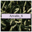
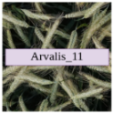
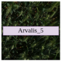
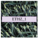
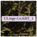
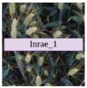
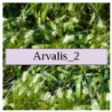
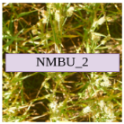
We also use two sets of $\Psi$ and $\Gamma$ as the internal and external test sets, as introduced by Najafian et al. [7]. The set $\Psi$ comprises 100 image frames, which were randomly selected from a video clip of a wheat field and have been manually annotated to serve as an internal test set. The set $\Gamma$ represents a subset of 365 manually annotated images from the GWHD dataset [23], which includes images from five countries and spans 18 domains, covering various growth stages of wheat.

2.2. Model Architecture

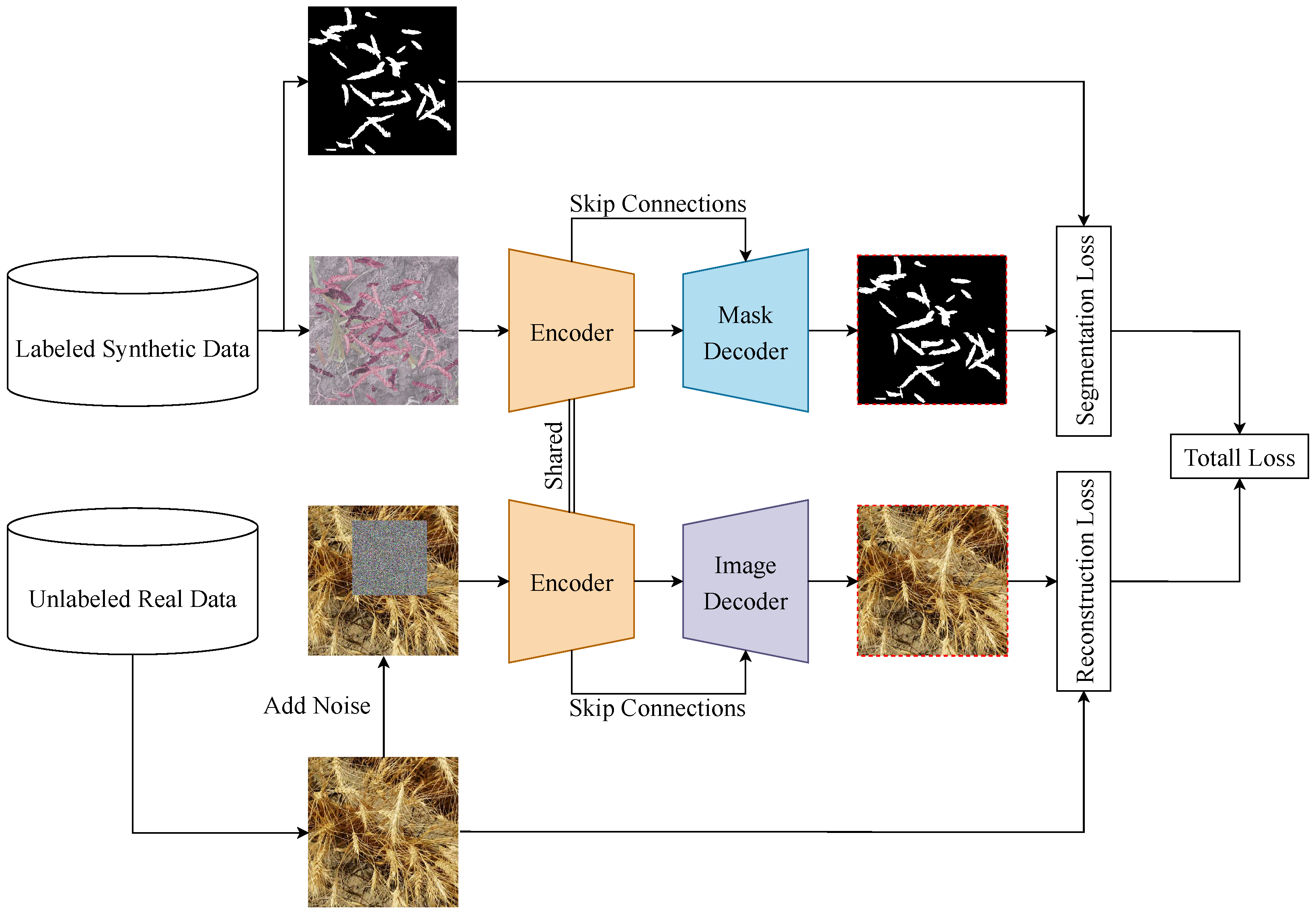
Figure 3 illustrates the convolutional neural network (CNN)-based model architecture employed in this research. This architecture is designed to facilitate representation learning through a diffusion process, in addition to performing the primary task of segmentation. The segmentation task is executed using computationally synthesized images along with their corresponding masks. Meanwhile, the representation learning aspect enables adaptation to real images using solely unannotated data, thereby reducing the reliance on manual annotation.

We use an encoder to develop a joint representation of both synthesized and real images. Additionally, the model architecture comprises an image decoder and a mask decoder. The former is designed to reconstruct the image from the output of the encoder, thereby enforcing learning features from real images. On the other hand, the mask decoder is tasked with developing a segmentation mask given the output of the encoder.

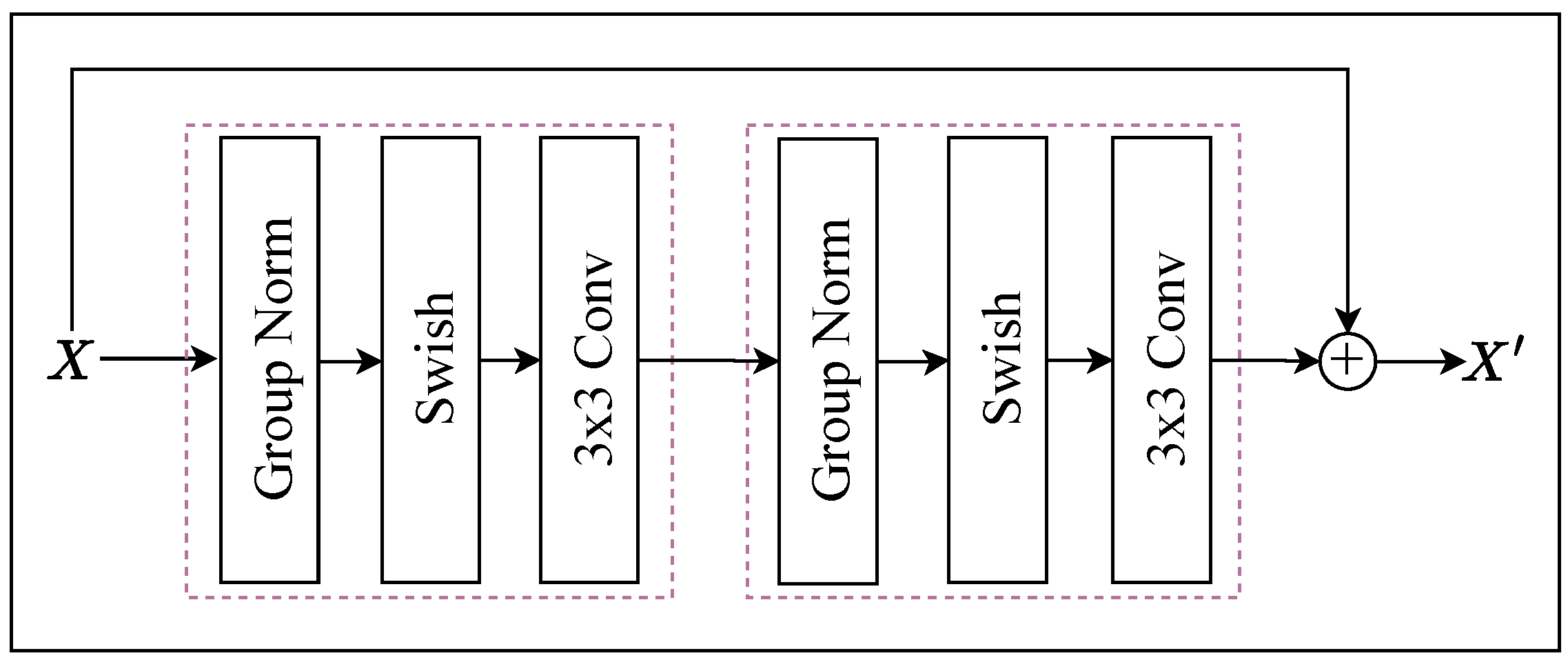
In implementing the encoder and decoders, we leveraged residual building blocks [24], each comprising two pairs of convolution and GroupNorm layers, supported by the Swish activation function [25] and integrated skip connections. Figure 4 shows a residual building block.

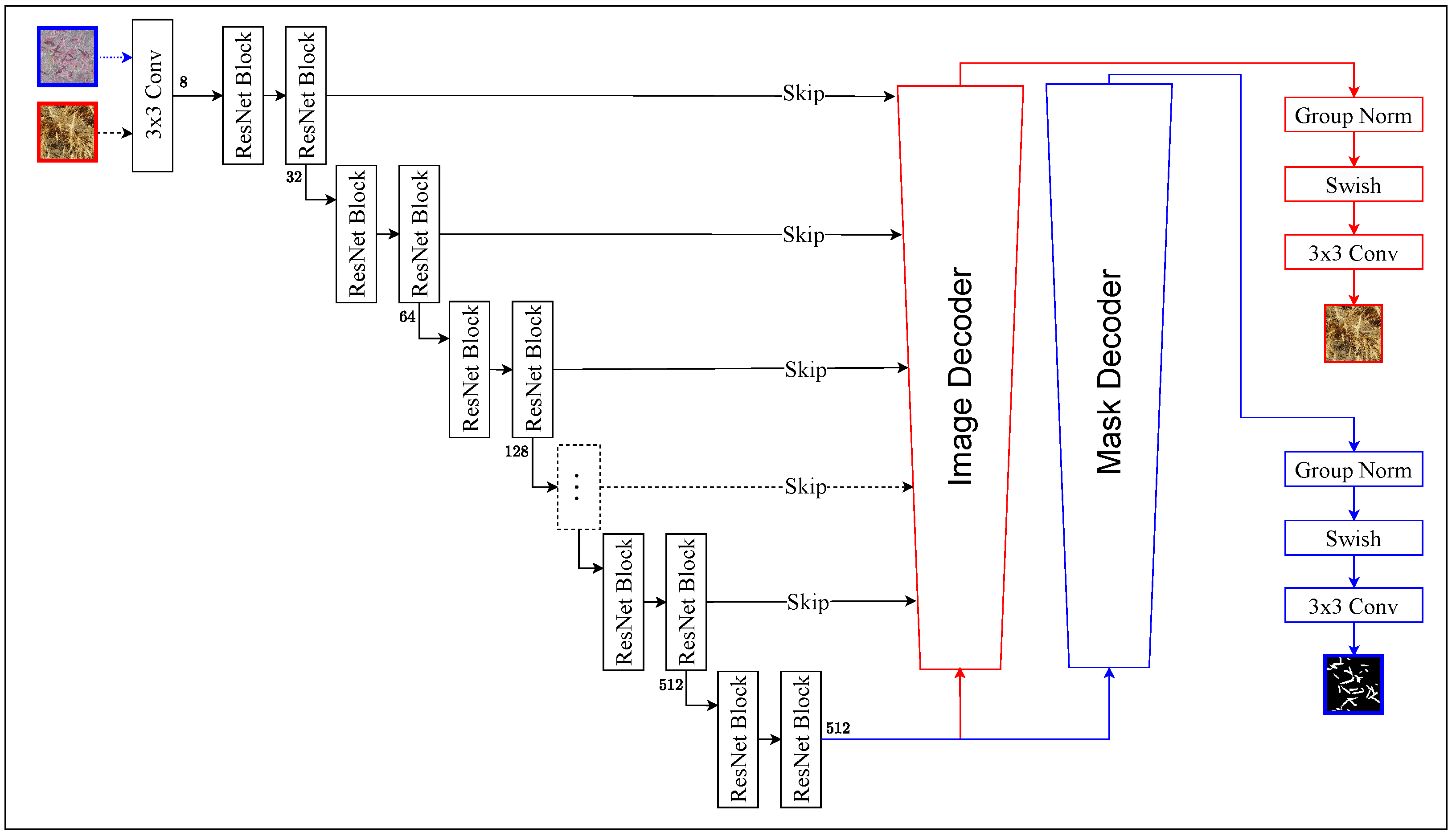
Figure 5 illustrates the encoder, consisting of one convolutional layer followed by 12 ResNet building blocks organized in six levels. Additionally, two skip-connection-free ResNet blocks serve as the network bottleneck. Moreover, down-sampling operations are performed after each pair of ResNet blocks using a convolution layer with a kernel size of three and a stride of two. The Swish activation function [25] is also consistently applied as the non-linearity across the encoder layers.

Synthetic images undergo a series of image augmentations [26]; then, they are fed into the encoder. The outputs of the encoder are subsequently passed to a mask decoder to generate accurate masks corresponding to the input images. To calculate the segmentation error, we use a linear combination of binary cross entropy (BCE) loss [27] and Dice loss [27] (see Equation (8)).

$$\begin{array}{c}{\mathcal{L}}_{BCE}=-\frac{1}{B\times N}\sum _{j=1}^B\sum _{i=1}^N\left(y_{i}log\left({\widehat{y}}_i\right)+(1-y_i)log(1-{\widehat{y}}_i)\right)\\ {\mathcal{L}}_{\mathit{Dice}}=1-\frac{2}{B}\sum _{j=1}^B\left(\frac{|M_j^s\cap {\widehat{M}}_j^s|}{|M_j^s|+|{\widehat{M}}_j^s|}\right)\\ {\mathcal{L}}_{Seg}={\lambda }_{BCE}\times {\mathcal{L}}_{BCE}+{\lambda }_{Dice}\times {\mathcal{L}}_{Dice}\end{array}$$

(8)

where $y_i$ is the true label of the pixel i, with a value of 1 if the pixel belongs to a wheat head and 0 otherwise. ${\widehat{y}}_i$ represents the model prediction of whether pixel i is from a wheat head. N is the number of pixels per image, and B is the batch size. $M_j^s$ is the ground truth mask for the synthetic image $I_j^s$, and ${\widehat{M}}_j^s$ is the model prediction for $I_j^s$.

We also generate noise-augmented images by applying Gaussian noise to the real image $I_j$ over t$(1\le t\le T)$ timesteps, as detailed in Equation (7). These noise-augmented images are subsequently routed through the encoder, followed by the image decoder, aiming to reconstruct the original images. The error for this branch is calculated by comparing the original image with the reconstructed image using a linear combination of MSE [28], SSIM [29], and a perceptual loss function [30]. The perceptual loss function calculates the mean absolute error between the pretrained ResNet18 output feature maps for the original image $I_j$ and the reconstructed image ${\widehat{I}}_j$. We used the $ResNet18\_Weights.IMAGENET1K\_V1$ weights from the Torchvision Python package [31]. We used the feature maps generated by the convolutional layer before the final average pooling layer of the ResNet18 model.

$$\begin{array}{c}{\mathcal{L}}_{\mathit{MSE}}=\frac{1}{B\times N}\sum _{j=1}^B\sum _{i=1}^N{(x_{ji}-{\widehat{x}}_{ji})}^2\\ {\mathcal{L}}_{\mathit{SSIM}}(I_j,{\widehat{I}}_j)=1-\frac{(2{\mu }_{I_j}{\mu }_{{\widehat{I}}_j}+c_1)(2{\sigma }_{I_j{\widehat{I}}_j}+c_2)}{({\mu }_{I_j}^2+{\mu }_{{\widehat{I}}_j}^2+c_1)({\sigma }_{I_j}^2+{\sigma }_{{\widehat{I}}_j}^2+c_2)}\\ {\mathcal{L}}_{\mathit{Perceptual}}=\frac{1}{B}\sum _{j=1}^B{∥\theta \left(I_j\right)-\theta \left({\widehat{I}}_j\right)∥}_2^2\\ {\mathcal{L}}_{Rec}={\lambda }_{MSE}\times {\mathcal{L}}_{MSE}+{\lambda }_{SSIM}\times {\mathcal{L}}_{SSIM}+{\lambda }_{Perceptual}\times {\mathcal{L}}_{Perceptual}\end{array}$$

(9)

where B is batch size; N is the number of pixels in an image $I_j$; $x_{ji}$ is the actual value of the i-th pixel of $I_j$; ${\widehat{x}}_{ji}$ is the predicted value for the i-th pixel of $I_j$; ${\mu }_{I_j}$ and ${\mu }_{{\widehat{I}}_j}$ are the mean intensity values of images $I_j$ and ${\widehat{I}}_j$, respectively; ${\sigma }_{I_j}^2$ and ${\sigma }_{{\widehat{I}}_j}^2$ are the variances of images $I_j$ and ${\widehat{I}}_j$, respectively; ${\sigma }_{I_j{\widehat{I}}_j}$ is the covariance between images $I_j$ and ${\widehat{I}}_j$; and $c_1$ and $c_2$ are constants introduced to stabilize the division. $\theta \left(I_j\right)$ and $\theta \left({\widehat{I}}_j\right)$ are ResNet18 features extracted from images $I_j$ and $\widehat{I_j}$, respectively.

These losses focus on variations between the reconstructed image and the original noise-free image from different perspectives: MSE loss focuses on pixel-level variations, SSIM loss focuses on local variations, and perceptual loss focuses on high-level global variations. The reconstruction loss is calculated as a linear combination of these loss functions, as described in Equation (9), where ${\lambda }_{MSE}$, ${\lambda }_{SSIM}$, and ${\lambda }_{Perceptual}$ are constant values and model hyperparameters.

2.3. Model Training and Evaluation

Considering the size of the datasets, we train our models over a total of 50 training epochs. For each epoch, we iterate over all the data in the datasets. At each iteration, we select a batch of 32 synthesized image–mask pairs and a separate batch of 32 real images from our datasets. The image–mask pairs are fed into the segmentation branch of our model, which consists of an encoder and a mask decoder. The segmentation loss is then calculated according to Equation (8). Similarly, the real images are fed into the reconstruction branch of our model, comprising the encoder (shared with the segmentation branch) and an image decoder, where the reconstruction loss is calculated as per Equation (9). The total loss is computed by summing the segmentation loss and the reconstruction loss. Figure 3 illustrates this process.

This dual-stream approach ensures that the encoder effectively attends to both types of data, with each decoder specializing in a task corresponding to its branch—namely, segmentation or reconstruction. Model updates are orchestrated using the AdamW optimizer [32], with the learning rate set at $0.0001$. For all experiments, the coefficients ${\lambda }_{MSE}$, ${\lambda }_{SSIM}$, ${\lambda }_{Perceptual}$, ${\lambda }_{BCE}$, and ${\lambda }_{Dice}$ are set to 1. After training for 50 epochs, we selected the model with the highest Dice score as the best model. During the evaluation process, we assessed the model performance using the Dice score and IoU. As a baseline for comparison, we used a model developed in [7].

3. Results

Table 1. The performance of the trained models was evaluated on our internal and external test sets using the IoU and Dice scores. Model ${\mathcal{F}}_{\eta +{\rho }_1}$ was trained on ${\mathbb{D}}_{\eta }$ and ${\mathbb{D}}_{{\rho }_1}$ and model ${\mathcal{F}}_{\eta +\zeta +\rho }$ is the result of fine-tuning model ${\mathcal{F}}_{\eta +{\rho }_1}$ on datasets ${\mathbb{D}}_{\eta +\zeta }$ and ${\mathbb{D}}_{\rho }$. We also compared the performance of these two models with the model developed in [7]. All of these models rely exclusively on synthesized image–mask pairs and/or unannotated images.

Model	Evaluation Method	Dice	IoU
$\mathcal{S}$ [7]	Internal test set $\Psi$	0.709	0.565
${\mathcal{F}}_{\eta +{\rho }_1}$	Internal test set $\Psi$	0.773	0.638
${\mathcal{F}}_{\eta +\zeta +\rho }$	Internal test set $\Psi$	0.807	0.686
S [7]	External test set $\Gamma$	0.367	0.274
${\mathcal{F}}_{\eta +{\rho }_1}$	External test set $\Gamma$	0.551	0.427
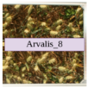
${\mathcal{F}}_{\eta +\zeta +\rho }$	External test set $\Gamma$	0.648	0.526

presents a quantitative evaluation of the performance of our developed models, namely, model ${\mathcal{F}}_{\eta +{\rho }_1}$ trained on ${\mathbb{D}}_{\eta }$ and ${\mathbb{D}}_{{\rho }_1}$ and model ${\mathcal{F}}_{\eta +\zeta +\rho }$ trained on ${\mathbb{D}}_{\eta +\zeta }$ and ${\mathbb{D}}_{\rho }$. These models were trained using both synthesized image–mask pairs and unannotated real images extracted from video clips of wheat fields. The performance of the baseline model $\mathcal{S}$ from Najafian et al. [7] is also reported in Table 1. The results demonstrate that the developed models, ${\mathcal{F}}_{\eta +{\rho }_1}$ and ${\mathcal{F}}_{\eta +\zeta +\rho }$, consistently outperformed the baseline model $\mathcal{S}$. These models rely on computationally annotated synthetic images and real unannotated images extracted from the video frames of wheat fields.

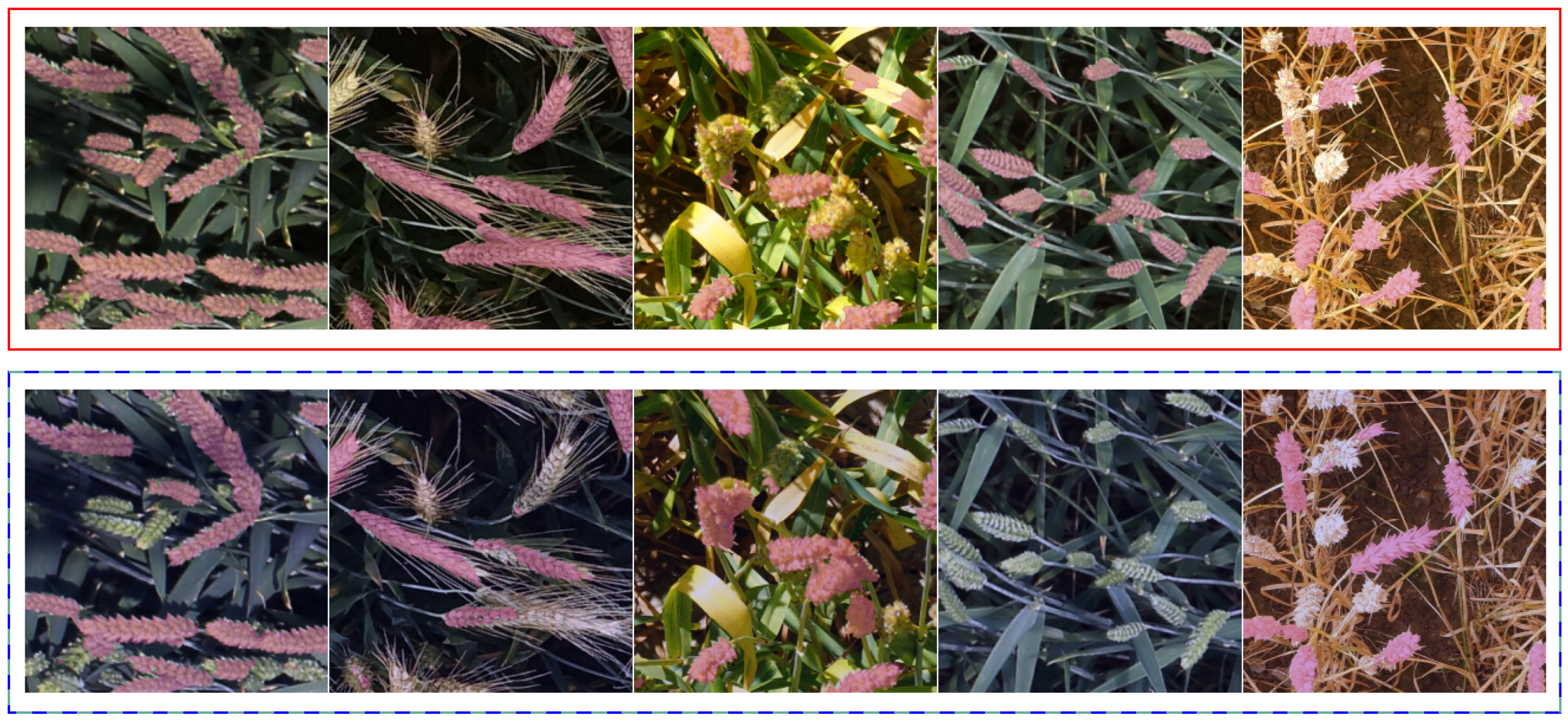
Figure 6 presents a qualitative evaluation of the performance of model ${\mathcal{F}}_{\eta +\zeta +\rho }$, identified as the best-performing model, and model $\mathcal{S}$ on several different domains. In general, model ${\mathcal{F}}_{\eta +\zeta +\rho }$ demonstrates superior performance compared to model $\mathcal{S}$. We also reported a case, as shown in the middle column, where model $\mathcal{S}$ performs better.

Table 2. The performance of the models on each of the 18 domains of the GWHD dataset. Model S, which was trained using the synthesized dataset, was reported in [7]. Model ${\mathcal{F}}_{\eta +{\rho }_1}$ was developed using dataset ${\mathbb{D}}_{\eta }$—consisting of 8000 computationally annotated synthesized images—and dataset ${\mathbb{D}}_{{\rho }_1}$, which includes 5296 unannotated real images. Model ${\mathcal{F}}_{\eta +\zeta +\rho }$ was developed using dataset ${\mathbb{D}}_{\eta +\zeta }$—consisting of 16,000 computationally annotated synthesized images—and dataset ${\mathbb{D}}_{\rho }$, which includes 10,592 unannotated real images. We trained model ${\mathcal{F}}_{\eta +{\rho }_1}$ from scratch, while model ${\mathcal{F}}_{\eta +\zeta +\rho }$ resulted from fine-tuning model ${\mathcal{F}}_{\eta +{\rho }_1}$ using dataset ${\mathbb{D}}_{\eta +\zeta }$ and dataset ${\mathbb{D}}_{\rho }$.

Domain	Model	Dice Score	Domain	Model	Dice Score
	$\mathcal{S}$	0.731		$\mathcal{S}$	0.711
	${\mathcal{F}}_{\eta +{\rho }_1}$	0.660		${\mathcal{F}}_{\eta +{\rho }_1}$	0.644
	${\mathcal{F}}_{\eta +\zeta +\rho }$	0.692		${\mathcal{F}}_{\eta +\zeta +\rho }$	0.759
	$\mathcal{S}$	0.848		$\mathcal{S}$	0.290
	${\mathcal{F}}_{\eta +{\rho }_1}$	0.815		${\mathcal{F}}_{\eta +{\rho }_1}$	0.193
	${\mathcal{F}}_{\eta +\zeta +\rho }$	0.857		${\mathcal{F}}_{\eta +\zeta +\rho }$	0.271
	$\mathcal{S}$	0.309		$\mathcal{S}$	0.601
	${\mathcal{F}}_{\eta +{\rho }_1}$	0.764		${\mathcal{F}}_{\eta +{\rho }_1}$	0.599
	${\mathcal{F}}_{\eta +\zeta +\rho }$	0.812		${\mathcal{F}}_{\eta +\zeta +\rho }$	0.769
	$\mathcal{S}$	0.240		$\mathcal{S}$	0.583
	${\mathcal{F}}_{\eta +{\rho }_1}$	0.503		${\mathcal{F}}_{\eta +{\rho }_1}$	0.795
	${\mathcal{F}}_{\eta +\zeta +\rho }$	0.431		${\mathcal{F}}_{\eta +\zeta +\rho }$	0.748
	$\mathcal{S}$	0.794		$\mathcal{S}$	0.156
	${\mathcal{F}}_{\eta +{\rho }_1}$	0.715		${\mathcal{F}}_{\eta +{\rho }_1}$	0.286
	${\mathcal{F}}_{\eta +\zeta +\rho }$	0.698		${\mathcal{F}}_{\eta +\zeta +\rho }$	0.356
	$\mathcal{S}$	0.389		$\mathcal{S}$	0.582
	${\mathcal{F}}_{\eta +{\rho }_1}$	0.479		${\mathcal{F}}_{\eta +{\rho }_1}$	0.492
	${\mathcal{F}}_{\eta +\zeta +\rho }$	0.605		${\mathcal{F}}_{\eta +\zeta +\rho }$	0.667
	$\mathcal{S}$	0.509		$\mathcal{S}$	0.884
	${\mathcal{F}}_{\eta +{\rho }_1}$	0.655		${\mathcal{F}}_{\eta +{\rho }_1}$	0.648
	${\mathcal{F}}_{\eta +\zeta +\rho }$	0.625		${\mathcal{F}}_{\eta +\zeta +\rho }$	0.805
	$\mathcal{S}$	0.859		$\mathcal{S}$	0.501
	${\mathcal{F}}_{\eta +{\rho }_1}$	0.674		${\mathcal{F}}_{\eta +{\rho }_1}$	0.488
	${\mathcal{F}}_{\eta +\zeta +\rho }$	0.671		${\mathcal{F}}_{\eta +\zeta +\rho }$	0.686
	$\mathcal{S}$	0.539		$\mathcal{S}$	0.629
	${\mathcal{F}}_{\eta +{\rho }_1}$	0.586		${\mathcal{F}}_{\eta +{\rho }_1}$	0.496
	${\mathcal{F}}_{\eta +\zeta +\rho }$	0.579		${\mathcal{F}}_{\eta +\zeta +\rho }$	0.520

presents the performance of the proposed models across various domains of the GWHD dataset. The results indicate that the proposed models generally outperform model $\mathcal{S}$ in most domains, exhibiting a lower variance and greater stability.

4. Discussion

Precision agriculture aims to integrate advanced technologies to address various challenges in the agricultural sector, enhancing productivity, efficiency, and profitability while minimizing waste and environmental impacts. Deep learning approaches play a crucial role in enabling automated decision-making capabilities. By automating the processing of visual data from agricultural fields, these decision-making processes can be significantly improved and scaled up.

However, the development of DL-based techniques encounters challenges stemming from the dynamic nature of agricultural fields, characterized by diverse growth stages, inconsistent weather conditions, and variable lighting. As such, models developed based on one snapshot of these fields are often not generalizable across different growth stages or environmental conditions. Furthermore, developing large-scale annotated datasets across various growth stages and environmental conditions is time-consuming and expensive. These challenges hinder the development of generalizable DL-based solutions for various agricultural tasks. Consequently, developing methodologies that allow DL-based solutions to generalize across different conditions (domains) could facilitate the widespread adoption of these technologies in the agricultural sector.

In response to these challenges, we developed a semi-self-supervised domain adaptation technique that employs deep convolutional neural networks and a probabilistic diffusion process. This approach was developed with minimal data annotation, requiring only three manually annotated images. We classify this method as semi-supervised because it leverages a small amount of annotated data (three images) alongside a significant volume of unannotated data. Additionally, this method can be considered as self-supervised as it utilizes computationally annotated data for model development.

The proposed model demonstrated substantial improvements in performance compared to the baseline model presented in recent work by Najafian et al. [7], while also showing a lower variance in model performance across 18 different domains from the GWHD dataset. These 18 domains represent various growth stages of wheat fields and different environmental conditions.

In this study, we devised a two-phase model training process. Initially, model ${\mathcal{F}}_{\eta +{\rho }_1}$ was developed by synthesizing a large number of computationally annotated samples resulting from a single sample for image synthesis and validation, showcasing a nearly $20\%$ improvement over a recent work by Najafian et al. [7] on the target domain. Subsequently, in the second phase, model ${\mathcal{F}}_{\eta +\zeta +\rho }$ leveraged additional computationally generated data, further enhancing the performance difference to $28\%$.

As presented in Table 1, our final model, ${\mathcal{F}}_{\eta +\zeta +\rho }$, shows a $28.1\%$ improvement in the Dice score and a $25.2\%$ improvement in the IoU when compared to model $\mathcal{S}$ from Najafian et al. The increased performance showcases the utility of the proposed semi-self-supervised domain adaptation technique.

Label noise poses a significant challenge in semi-supervised domain adaptation, whether it stems from manual annotation errors or errors introduced by the use of non-curated pseudo-labeled data for model fine-tuning. The presence of label noise in manually annotated data can severely degrade the performance of deep learning models by introducing incorrect information during the training phase, leading to suboptimal decision boundaries and poor generalization to the target domain. Utilizing pseudo-labels without any form of curation may also further exacerbate this issue, as these uncurated labels can propagate errors and amplify the negative impact of label noise. Adopting systematic approaches, such as the Label Recovery and Trajectory Designable Network (LRTDN) proposed by Yang et al. [33], could alleviate this challenge. The LRTDN aims to address the noise in pseudo-labels by incorporating a robust annotation check module that identifies and corrects label anomalies, thereby enhancing the reliability of the training data. This ensures that the model learns from more accurate labels, ultimately improving its performance in the presence of annotation noise.

In agricultural fields, pixel-level annotation poses unique challenges. The presence of many small regions of interest, such as wheat heads, necessitates meticulous annotation. Moreover, the lack of contrast between these regions and the background further complicates the task. For instance, accurately differentiating wheat heads from the background requires significant attention and accuracy during manual annotation. Consequently, pixel-level accurate annotation of a single image may take several hours, making developing large-scale, pixel-level, accurately annotated images costly and tedious. Furthermore, agricultural data are substantially variable due to variations in environmental conditions, phenotypic varieties, and crop growth stages. As such, it is impractical to develop a large-scale annotated dataset that represents all these variations across the crop’s lifecycle. By utilizing only a small number of manually annotated images from the target domain, the proposed method accelerates the development of deep learning models for various fields. Additionally, the resulting model could facilitate the development of further annotated samples from the target domain by making predictions using the initial model for samples from the target domain and then applying corrections if needed. This semi-automated approach substantially accelerates the creation of annotated samples from the target domain that could be used to further improve the performance of the developed model in the target domain.

In this research, we adopted an extreme strategy by utilizing only two annotated images for training and one for validation. However, we recommend incorporating more manually annotated samples from diverse domains to further enhance the robustness of the proposed approach. Additionally, in this research, we primarily relied on default hyperparameters. Tuning the model hyperparameters could lead to further improvements in model performance.

5. Conclusions

This research introduces a semi-self-supervised domain adaptation methodology characterized by a dual-stream encoder–decoder model architecture, specifically designed for the downstream task of semantic segmentation of wheat heads. We synthesized a large-scale, computationally annotated dataset from three manually annotated images. We also used unannotated image frames extracted from wheat field videos captured at two different growth stages. The model architecture and training strategy, utilizing both image segmentation and reconstruction, were strategically designed to mitigate the challenges associated with domain shifts while minimizing the need for extensive data annotation. The external evaluation of our proposed approach on a subset of the GWHD dataset demonstrated a substantial improvement in model performance over a recent work. This underscores the utility of our proposed approach in alleviating domain shift, allowing for the development of generalizable models with minimal manual data annotation, which, in turn, could enable the widespread adoption of DL-based approaches in the agricultural sector.

References

1. Oliver, M.A.; Bishop, T.F.; Marchant, B.P. Precision Agriculture for Sustainability and Environmental Protection; Routledge: Abingdon, UK, 2013. [Google Scholar]
2. Tan, M.; Le, Q. EfficientNet: Rethinking Model Scaling for Convolutional Neural Networks. In Proceedings of the International Conference on Machine Learning, Long Beach, CA, USA, 9–15 June 2019; pp. 6105–6114. [Google Scholar]
3. Najafian, K.; Jin, L.; Kutcher, H.R.; Hladun, M.; Horovatin, S.; Oviedo-Ludena, M.A.; De Andrade, S.M.P.; Wang, L.; Stavness, I. Detection of Fusarium Damaged Kernels in Wheat Using Deep Semi-Supervised Learning on a Novel WheatSeedBelt Dataset. In Proceedings of the IEEE/CVF International Conference on Computer Vision, Paris, France, 2–6 October 2023; pp. 660–669. [Google Scholar]
4. Wang, C.Y.; Bochkovskiy, A.; Liao, H.Y.M. YOLOv7: Trainable bag-of-freebies sets new state-of-the-art for real-time object detectors. In Proceedings of the IEEE/CVF Conference on Computer Vision and Pattern Recognition, Vancouver, BC, Canada, 17–24 June 2023; pp. 7464–7475. [Google Scholar]
5. Najafian, K.; Ghanbari, A.; Stavness, I.; Jin, L.; Shirdel, G.H.; Maleki, F. A Semi-Self-Supervised Learning Approach for Wheat Head Detection using Extremely Small Number of Labeled Samples. In Proceedings of the IEEE/CVF International Conference on Computer Vision, Virtual, 11–17 October 2021; pp. 1342–1351. [Google Scholar]
6. Mo, Y.; Wu, Y.; Yang, X.; Liu, F.; Liao, Y. Review the state-of-the-art technologies of semantic segmentation based on deep learning. Neurocomputing 2022, 493, 626–646. [Google Scholar] [CrossRef]
7. Najafian, K.; Ghanbari, A.; Sabet Kish, M.; Eramian, M.; Shirdel, G.H.; Stavness, I.; Jin, L.; Maleki, F. Semi-Self-Supervised Learning for Semantic Segmentation in Images with Dense Patterns. Plant Phenomics 2023, 5, 0025. [Google Scholar] [CrossRef] [PubMed]
8. Kirillov, A.; Mintun, E.; Ravi, N.; Mao, H.; Rolland, C.; Gustafson, L.; Xiao, T.; Whitehead, S.; Berg, A.C.; Lo, W.Y.; et al. Segment Anything. arXiv 2023, arXiv:2304.02643. [Google Scholar]
9. He, K.; Gkioxari, G.; Dollár, P.; Girshick, R. Mask R-CNN. In Proceedings of the 2017 IEEE International Conference on Computer Vision (ICCV), Venice, Italy, 22–29 October 2017; pp. 2980–2988. [Google Scholar] [CrossRef]
10. Hafiz, A.M.; Bhat, G.M. A survey on instance segmentation: State of the art. Int. J. Multimed. Inf. Retr. 2020, 9, 171–189. [Google Scholar] [CrossRef]
11. Champ, J.; Mora-Fallas, A.; Goëau, H.; Mata-Montero, E.; Bonnet, P.; Joly, A. Instance segmentation for the fine detection of crop and weed plants by precision agricultural robots. Appl. Plant Sci. 2020, 8, e11373. [Google Scholar] [CrossRef] [PubMed]
12. Sinha, S.; Gehler, P.; Locatello, F.; Schiele, B. TeST: Test-Time Self-Training Under Distribution Shift. In Proceedings of the IEEE/CVF Winter Conference on Applications of Computer Vision (WACV), Waikoloa, HI, USA, 2–7 January 2023; pp. 2759–2769. [Google Scholar]
13. Hu, Q.; Guo, Y.; Xie, X.; Cordy, M.; Papadakis, M.; Ma, L.; Le Traon, Y. CodeS: Towards code model generalization under distribution shift. In Proceedings of the International Conference on Software Engineering (ICSE): New Ideas and Emerging Results (NIER), Melbourne, Australia, 14–20 May 2023. [Google Scholar]
14. Hwang, D.; Misra, A.; Huo, Z.; Siddhartha, N.; Garg, S.; Qiu, D.; Sim, K.C.; Strohman, T.; Beaufays, F.; He, Y. Large-scale ASR Domain Adaptation using Self- and Semi-supervised Learning. In Proceedings of the ICASSP 2022—2022 IEEE International Conference on Acoustics, Speech and Signal Processing (ICASSP), Singapore, 23–27 May 2022; pp. 6627–6631. [Google Scholar]
15. Pan, F.; Shin, I.; Rameau, F.; Lee, S.; Kweon, I.S. Unsupervised Intra-domain Adaptation for Semantic Segmentation through Self-Supervision. In Proceedings of the IEEE/CVF Conference on Computer Vision and Pattern Recognition, Seattle, WA, USA, 14–19 June 2020; pp. 3764–3773. [Google Scholar]
16. Rani, V.; Nabi, S.T.; Kumar, M.; Mittal, A.; Kumar, K. Self-supervised Learning: A Succinct Review. Arch. Comput. Methods Eng. 2023, 30, 2761–2775. [Google Scholar] [CrossRef] [PubMed]
17. Zbontar, J.; Jing, L.; Misra, I.; LeCun, Y.; Deny, S. Barlow Twins: Self-Supervised Learning via Redundancy Reduction. In Proceedings of the 38th International Conference on Machine Learning, Virtual Event, 18–24 July 2021; Meila, M., Zhang, T., Eds.; Proceedings of Machine Learning Research (PMLR). Volume 139, pp. 12310–12320. [Google Scholar]
18. Ramesh, A.; Dhariwal, P.; Nichol, A.; Chu, C.; Chen, M. Hierarchical Text-Conditional Image Generation with CLIP Latents. arXiv 2022, arXiv:2204.06125. [Google Scholar]
19. Rombach, R.; Blattmann, A.; Lorenz, D.; Esser, P.; Ommer, B. High-Resolution Image Synthesis with Latent Diffusion Models. In Proceedings of the IEEE/CVF Conference on Computer Vision and Pattern Recognition, New Orleans, LA, USA, 18–24 June 2022; pp. 10684–10695. [Google Scholar]
20. Croitoru, F.A.; Hondru, V.; Ionescu, R.T.; Shah, M. Diffusion Models in Vision: A Survey. IEEE Trans. Pattern Anal. Mach. Intell. 2023, 45, 10850–10869. [Google Scholar] [CrossRef] [PubMed]
21. Chen, T. On the Importance of Noise Scheduling for Diffusion Models. arXiv 2023, arXiv:2301.10972. [Google Scholar]
22. Nichol, A.Q.; Dhariwal, P. Improved Denoising Diffusion Probabilistic Models. In Proceedings of the International Conference on Machine Learning. PMLR, Virtual Event, 18–24 July 2021; pp. 8162–8171. [Google Scholar]
23. David, E.; Serouart, M.; Smith, D.; Madec, S.; Velumani, K.; Liu, S.; Wang, X.; Pinto, F.; Shafiee, S.; Tahir, I.S.; et al. Global Wheat Head Detection 2021: An Improved Dataset for Benchmarking Wheat Head Detection Methods. Plant Phenomics 2021, 22, 9846158. [Google Scholar] [CrossRef] [PubMed]
24. He, K.; Zhang, X.; Ren, S.; Sun, J. Deep Residual Learning for Image Recognition. In Proceedings of the IEEE Conference on Computer Vision and Pattern Recognition, Las Vegas, NV, USA, 27–30 June 2016; pp. 770–778. [Google Scholar]
25. Ramachandran, P.; Zoph, B.; Le, Q.V. Searching for Activation Functions. arXiv 2017, arXiv:1710.05941. [Google Scholar]
26. Buslaev, A.; Iglovikov, V.I.; Khvedchenya, E.; Parinov, A.; Druzhinin, M.; Kalinin, A.A. Albumentations: Fast and flexible image augmentations. Information 2020, 11, 125. [Google Scholar] [CrossRef]
27. Wazir, S.; Fraz, M.M. HistoSeg: Quick attention with multi-loss function for multi-structure segmentation in digital histology images. In Proceedings of the 2022 12th International Conference on Pattern Recognition Systems (ICPRS), Saint-Etienne, France, 7–10 June 2022; pp. 1–7. [Google Scholar]
28. Beheshti, S.; Hashemi, M.; Sejdic, E.; Chau, T. Mean Square Error Estimation in Thresholding. IEEE Signal Process. Lett. 2010, 18, 103–106. [Google Scholar] [CrossRef]
29. Hore, A.; Ziou, D. Image Quality Metrics: PSNR vs. SSIM. In Proceedings of the 2010 20th International Conference on Pattern Recognition, Istanbul, Turkey, 23–26 August 2010; pp. 2366–2369. [Google Scholar]
30. Johnson, J.; Alahi, A.; Fei-Fei, L. Perceptual Losses for Real-Time Style Transfer and Super-Resolution. In Proceedings of the Computer Vision–ECCV 2016: 14th European Conference, Amsterdam, The Netherlands, 11–14 October 2016; Proceedings, Part II 14. Springer: Cham, Switzerland, 2016; pp. 694–711. [Google Scholar]
31. Paszke, A.; Gross, S.; Massa, F.; Lerer, A.; Bradbury, J.; Chanan, G.; Killeen, T.; Lin, Z.; Gimelshein, N.; Antiga, L.; et al. PyTorch: An Imperative Style, High-Performance Deep Learning Library. In Proceedings of the Advances in Neural Information Processing Systems 32, Vancouver, BC, Canada, 8–12 December 2019; pp. 8024–8035. [Google Scholar]
32. Loshchilov, I.; Hutter, F. Decoupled Weight Decay Regularization. arXiv 2017, arXiv:1711.05101. [Google Scholar]
33. Yang, B.; Lei, Y.; Li, X.; Li, N.; Nandi, A.K. Label Recovery and Trajectory Designable Network for Transfer Fault Diagnosis of Machines with Incorrect Annotation. IEEE/CAA J. Autom. Sin. 2024, 11, 932–945. [Google Scholar] [CrossRef]
Figure 1. Three manually annotated image–mask pairs were utilized for data synthesis. We developed two training sets by synthesizing computationally annotated images using manually annotated images from the left ( I η ) and the middle ( I ζ ), producing 8000 images based on I η and 8000 images based on I ζ . Hereafter, we refer to the 8000 images developed based on I η as dataset D η . We refer to the set comprising the whole 16,000 images as D η + ζ . Additionally, we created a validation set by synthesizing 4000 images, with 2000 from the image on the right ( I τ ) and 2000 images based on I ζ . Hereafter, we refer to this set of 4000 images as D ζ + τ . Dataset D ζ + τ was made to allow for a balanced representation of wheat field images from the early and late growth stages. All computationally annotated samples were synthesized following the methodology described by Najafian et al. [7].
Algorithms 17 00267 g001
Figure 2. Examples of computationally synthesized images and their corresponding segmentation masks.
Algorithms 17 00267 g002
Figure 3. Schematic representation of the model architecture. The encoder focuses on developing a joint image representation for both synthesized and real images, while the mask decoder aims at generating segmentation masks and the image decoder aims at reconstructing the real images, forcing the encoder to adapt to the real images.
Algorithms 17 00267 g003
Figure 4. A ResNet block comprises three groups of operations, including convolution, GroupNorm layers, and the Swish activation function for nonlinearity. It also incorporates skip connections to enhance feature propagation.
Algorithms 17 00267 g004
Figure 5. Encoder model architecture designed by combining convolutional layers, ResNet blocks, and GroupNorm layers. Also, in each of the two decoding streams, we utilize concatenation instead of addition.
Algorithms 17 00267 g005
Figure 6. Showcasing the prediction performance of model F η + ζ + ρ (highlighted in a red box in the upper row) in comparison with the results obtained by model S [7] (highlighted in a blue box in the lower row) on samples from the Global Wheat Head Detection dataset [23].
Algorithms 17 00267 g006