Abstract
This study focuses on generating reliable signals from measured noisy signals through an enhanced sensor fusion method. The main contribution of this research is the development of a novel sensor fusion architecture that creates virtual sensors, improving the system’s redundancy. This architecture utilizes an input observer to estimate the system input, then it is introduced to the system model, the output of which is the virtual sensor. Then, this virtual sensor includes two filtering stages, both derived from the system’s dynamics—the input observer and the system model—which effectively diminish noise in the virtual sensors. Afterwards, the same architecture includes a classical sensor fusion scheme and a voter to merge the virtual sensors with the real measured signals, enhancing the signal reliability. The effectiveness of this method is shown by applying merged signals to two distinct diagnosers: one utilizes a high-order sliding mode observer, while the other employs an innovative extension of a predefined-time observer. The findings indicate that the proposed architecture improves diagnostic results. Moreover, a three-wheeled omnidirectional mobile robot equipped with noisy sensors serves as a case study, confirming the approach’s efficacy in an actual noisy setting and highlighting its principal characteristics. Importantly, the diagnostic systems can manage several simultaneous actuator faults.
1. Introduction
Modern industrial processes and systems are becoming larger and more complex, demanding high reliability and performance from the system [1]. To meet these demands, modern systems incorporate sophisticated control and decision-making structures, including fault diagnosis and recovery stages, to exhibit intelligent behavior even under abnormal conditions.
Regarding fault diagnosis [2,3,4], this stage deals with abnormal behaviors (faults) by detecting, locating, and identifying them. The output of this stage can either alert human operators, or be used by a fault-tolerant system with the aim of removing hazardous situations. One of the most widely reported approaches in fault diagnosis is the fault model-based approach [5,6,7], where the observers, who are the core group focused on generating results [1,2], are used to determine the existence of faults. All previously mentioned results assume that the input signal is sufficiently free of noise; however, this assumption rarely hold in real situations, limiting the use of sophisticated diagnosers. In particular, the proposed diagnoser in those works are based on asymptotic observers or finite-time observers. When noise is considered, the performance of such diagnosers is reduced, producing false fault detection. In other words, the accuracy of diagnosers depends on the reliability of the measured signals; nevertheless, in many real cases the sensor noise limits the reliability of such information.
This problem is overcome by using sensor fusion algorithms [8,9,10,11]; unfortunately, in many cases there are not enough different sensors to use such algorithms. Moreover, the system sensors may be measuring signals which are not comparable with each other, which may make merging them with a sensor fusion technique difficult. To avoid this last drawback, in the literature changing the sensor coordinates has been proposed [12,13]; regrettably this strategy is limited to very particular cases.
This work proposes a novel sensor fusion architecture capable of generating several virtual sensors comparable with each other. These are merged in a sensor fusion stage to obtain more reliable output signals for subsequent processes, such as fault diagnosis, observers, and controllers. The idea behind the proposed architecture is to include two filter stages that generate feasible system inputs and outputs based on the system model, significantly reducing signal noise. Additionally, a voter enhances the reliability of virtual sensor signals by selecting those with the minimum variance.
To show the efficiency of the proposed architecture, its output is used by two diagnosers, one based on a high-order sliding mode (HOSM) observer, and the other based on an enhanced predefined-time observer herein introduced. Both cases show that when the proposed architecture is used, the efficiency of the diagnosers is improved, i.e., the false positive/negative fault detections are reduced, and the fault diagnosis is improved.
This work is organized as follows. Section 2 introduces the sensor fusion architecture, emphasizing how from a subset of output signals and using an input observer scheme, the virtual sensors may be implemented. This section also introduces a novel diagnoser based on an enhanced predefined-time observer. Section 3 introduces a three-wheeled omnidirectional mobile robot, that is the real system on which the proposed architecture and diagnosers are tested. Section 4 shows the experiments and the derived results. All of them show that the use of the proposed architecture improves the diagnosis of faults. Finally, the conclusions are presented.
2. Sensor Fusion Architecture
Figure 1 depicts the proposed sensor fusion architecture and the diagnoser. In the proposed approach, each virtual sensor gives an estimate of the entire set of measured system outputs, and every virtual sensor is merged, using a classical fusion stage, with the measured system output generating a cleaner estimated signal. Afterwards, a voter is used to select the most reliable estimated signal. This single output of the architecture is a reliable estimate of the system output that may be used by a diagnoser or any other device demanding reliable measures of the system. It is worth remarking that every virtual sensor is generated from a subset of the system outputs using an element that we name a homogenizer.

Figure 1.
Sensor fusion architecture and the diagnoser applied in a diagnoser scheme. The sensor fusion architecture encompasses the homogenizer, EKF, and voter stages. The homogenizer generates virtual outputs, while the EKF merges real and virtual signals to generate more reliable signals, the filter reduces the noise from the signals, and the voter selects the best signal (in this work, the minimum variance signal). The diagnoser leverages these reliable signals to detect, locate, and identify concurrent and nonconcurrent faults.
This fusion architecture generates more reliable signals, allowing the use of sophisticated diagnosers (such as those based on sliding modes) capable of diagnosing faults in a short period of time after their occurrence, and drastically reducing the number of false fault detections.
Since in this work the output of the proposed fusion architecture is used by a fault diagnoser, we considered the system model introduced in [14]:
where the state is , the control input is , the output is , and the fault magnitude is , while , , , and are smooth functions defined on an open set .
Assumption 1.
No one belongs to the kernel of . In other words, any fault occurrence always affects the system state.
2.1. Sensor Fusion Architecture
The proposed sensor fusion architecture is composed of the signal homogenizer, sensor fusion, and filter stages.
2.1.1. Homogenizer
Modern systems are endowed with several sensors grouped into different classes depending on the type of measured signals. The information provided by sensors, although different in nature, may be redundant. For example, autonomous vehicles include cameras, GPS, lidar, encoders, among other sensors, that register different types of information. For example, the GPS gives information related to the vehicle’s position and orientation, whereas the encoders measure the motors’ positions and velocities. Nevertheless, the information provided by encoders and GPS may be redundant when direct or inverse kinematics are used. Our approach leverages system characteristics to add redundancy to the system information. To formalize these concepts, the following sets and maps are defined.
Definition 1.
Let be the set of system outputs, and be the system output vector. Let be two arbitrary subsets of Σ. If there exists a function such that from the information provided by the signals in , the signals in may be estimated, then is the i-th homogenizer for . The homogenizer value is named the i-th virtual sensor of . If , then , i.e., the whole set of output sensors is reconstructed from .
For example, assuming that the motor speed and position are measured in the system outputs and , respectively, then the homogenizer can be implemented by an integration procedure, adding a virtual sensor for the position.
Homogenizer may be implemented in several ways, depending on the relationship between signals in and . This work proposes the homogenizer depicted in Figure 2, that is based on the input estimator proposed in [15]. This is for dynamical systems under the assumption of observability when the system output is . For this, signals in are used to estimate the system input . Afterwards, leveraging and the system model, the system outputs , due to , are estimated, i.e., the proposed homogenizer is capable of computing all the signals in . Thus, the homogenizer is represented as a function . As a notation () is used to indicate that all system outputs are estimated from the information in . In addition to , the proposed homogenizer also computes the estimated state and the estimated input , obtained from .

Figure 2.
Implementation of the signal homogenizer i to obtain the virtual sensors , an estimate of the state , and an estimate for the input .
In order to compute the input , first, the coordinate transformation
is applied [15], where and is the internal system dynamic. Notice that corresponds to the coordinate transformation obtained from the a-th output , with . Then, by the construction of the coordinate transformation, the states and their derivatives can be estimated by higher-order sliding mode (HOSM) differentiators [16] (by computing the derivatives of the outputs of the system), where , and denotes the relative degree of the a-th output . Once the state and its derivative are estimated, the input is computed as reported in [15]:
where denotes the derivative of h along f, see [17], and the matrix can be constructed as [15]
Notice that the proposed homogenizer depicted in Figure 2 computes the system states from . Then, using the system model, the system output is estimated, generating virtual system outputs.
2.1.2. Sensor Fusion
The reliability of the values of the system signals in is increased if there exists at least one homogenizer . In this case, the system outputs y and the signals in are smartly merged by using an extended Kalman filter () to obtain a more accurate value of signals in [18]. Note that the EKF algorithm requires a discrete system, so the system in Equation (1) is discretized with the Euler method or any other discretization method. In addition, herein the subscript k is used to denote the discrete time index.
For the sensor fusion, the signals in the output vector y and the virtual sensors are arranged into an augmented measurement vector as follows [19]:
where is the vector formed with the virtual sensors . While the augmented covariance matrix of the measurement noise is given by
where is the covariance matrix of the noise of the real sensors’ measurements and is the covariance matrix of the noise of the virtual sensors obtained from the homogenizer i. The entries of the covariance matrix in Equation (5) are selected based on the respective measurement noise variance. Similarly, the entries of the process noise covariance matrix are chosen. Once the parameters of the are set, the standard EKF algorithm [20] is used to obtain the required sensor fusion.
2.1.3. Filter
The sensor fusion stage generates more reliable signals. These signals are filtered to reduce their noise even more. To this end, a classical second-order low pass filter (LPF) is used:
The parameters and are chosen such that a desired transient and noise reduction are achieved.
2.1.4. Voter
Finally, a voter selects the output of the sensor fusion architecture. This is depicted as the min operation in Figure 1. In this case, it selects the signals and , corresponding to the signal with the lowest variance.
2.2. Diagnoser
The naive approach of solving the unknown faults from Equation (1) and the estimated state (output from the proposed architecture) is not possible, since it involves the computation of , increasing the noise and leading to false faults detection. This inconvenience is avoided by using a fault diagnoser; in particular, this work proposes a diagnoser based on a predefined-time observer to swiftly diagnose the fault.
First, we assume that the estimated system state is partitioned as , where the states in are directly affected by the faults, i.e., when , and the states in are not affected by the faults, i.e., when ; then, from Equation (1) we obtain
The diagnoser is proposed as the following predefined-time observer:
where (that is related to the fault value) is the observer feedback law that must be selected to ensure that converges to at a predefined-time . The estimation error is
where the measurements of are in . The time derivative of the error in Equation (9) is
Proposition 1 shows how to compute . The proof of this proposition is based on the next theorem, presented in [21].
Theorem 1
([21]). Consider the nonlinear system
where the system state is , the system parameters are , which are assumed to be constant, and is assumed to be a continuous nonlinear function. If there exists a continuous definite-positive radially unbounded function such that
with constants , , and , and the constant γ is given by
where Γ is the gamma function [22], , and .
- Then, the origin of (11) is predefined-time stable with as its predefined time.
Proposition 1.
Let , where its i-th component is bounded by a positive constant, i.e., , . If the i-th entry of the observer feedback law Θ is chosen as
then, the origin of the error system (10) is predefined-time stable with as its predefined time.
Proof.
For every estimation error consider the continuous radially unbounded Lyapunov function , . The time derivative of each Lyapunov function yields
where is computed using Equation (13). Thus, by using Theorem 1, every is predefined-time stable, . Therefore, the origin of the error system (10) is predefined-time stable with as its predefined time. □
Since the origin of (10) is reached in a predefined time, it implies that , and for . Then, the equivalent observer feedback law is obtained such that holds. Hence, from Equation (10), is found as
So, if , , and Assumption 1 holds, then the estimation of the fault magnitudes can be computed from Equation (16) as
where the pseudoinverse exists by Assumption 1. In order to remove the high-frequency components of each estimated fault , due to the high-frequency signals of , second-order LPFs, such as the ones proposed in Section 2.1.3, are required:
where the filter settling time should be selected to be approximately equal to to ensure a fast convergence to the real fault .
3. Case Study
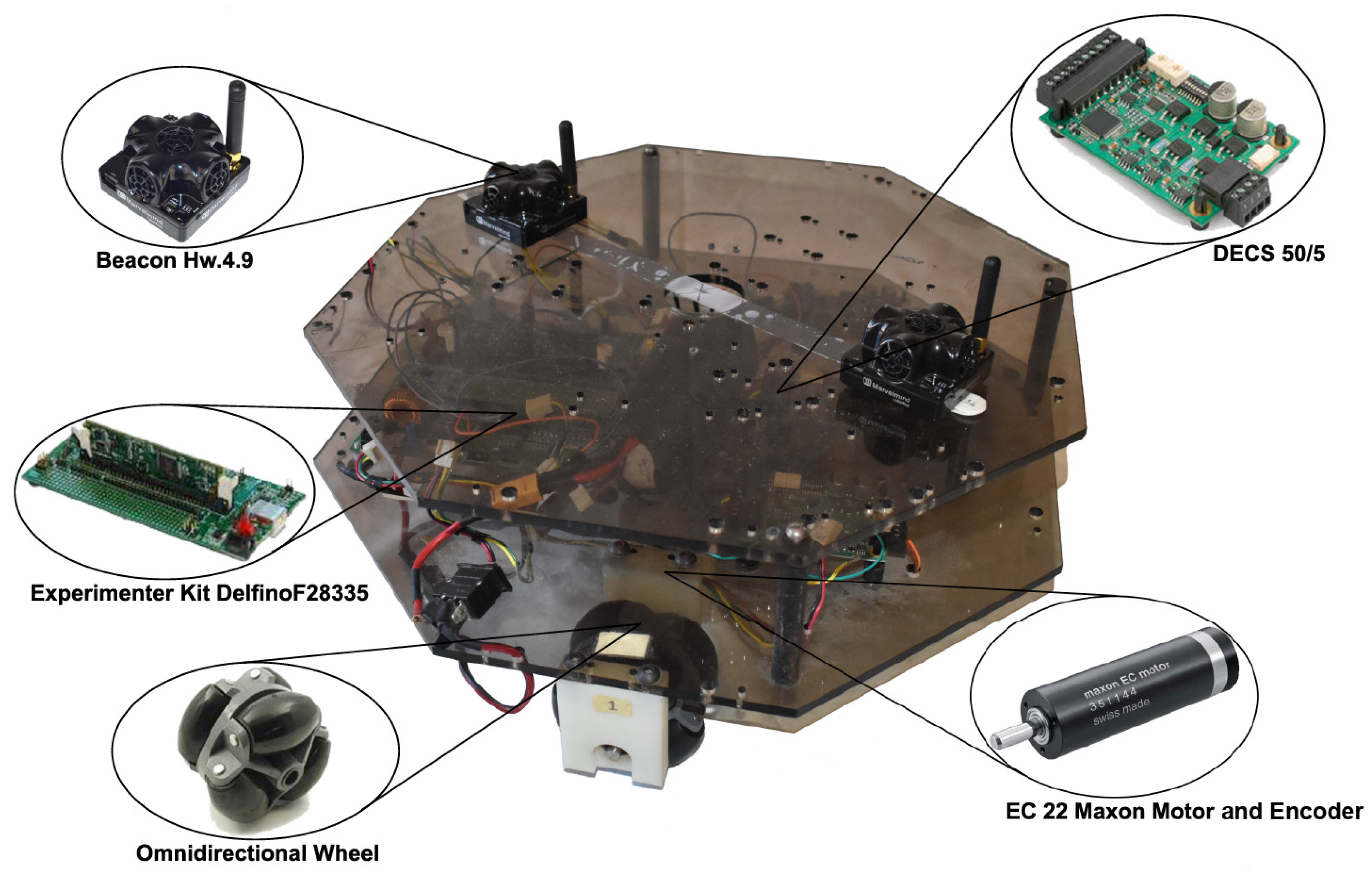
The three-wheeled omnidirectional mobile robot depicted in Figure 3 is considered for this case study.
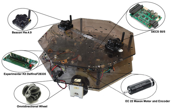
Figure 3.
Three-wheeled omnidirectional mobile robot.
3.1. Prototype
Our prototype, depicted in Figure 3, is a three-wheeled omnidirectional mobile robot. It has three omnidirectional wheels driven by EC 22 brushless Maxon motors connected to gearbox reducers with a ratio of 109:1. Each motor shaft speed and rotational direction is controlled by the Maxon DECS 50/5 driver. As a computational unit, the 32-bit Experimenter Kit Delfino F28335 Texas Instruments microcontroller is used.
The position and orientation of the mobile robot are measured by a Marvelmind Starter set HW 4.9 indoor GPS system, while every motor shaft velocity is obtained by Maxon encoders with a resolution of 512 counts per turn. The sensors have a frequency of 100 Hz and the sensors’ data are collected with a sampling time of 0.025 s.
3.2. Model of the Three-Wheeled Omnidirectional Mobile Robot
The state space representation of a three-wheeled omnidirectional mobile robot in global coordinates is taken from [23]; then, the motors’ dynamics are added such that the following state space model is derived:
where
the signals are the inputs to the system, represent the shaft velocity of the i-th motor, ; the states , , and are the positions at the coordinates (x, y), and the orientation of the mobile robot, respectively. While , are the mobile robot linear velocities , , respectively, and is the angular velocity of the vehicle about its center of mass. The states , , and represent the motor velocities (RPM). Since real motors have fast dynamics, the parameters , , and are chosen such that a fast convergence is achieved, whilst the parameter (RPM) is selected according to the datasheet of the motors. The other system parameters are identified by using the least squares approach in [24]. The derived parameters are reported in Table 1.

Table 1.
Identified parameters of the system.
3.3. Signal Homogenizer
The system output vector is , where the GPS output signals , , and , are the (X,Y) position in a global framework and the orientation of the mobile robot, respectively; the encoders’ output signals are , , and . Hence, the set of system outputs is . From the set , two subsets are generated: , which contains the GPS outputs; and for the encoder’s outputs.
In order to generate the homogenizers and , the structure depicted in Figure 2 is applied. For the homogenizer , the coordinate transformation is chosen as , , and . So, the estimated input (see Figure 2) is computed from Equation (2) as
where , , and their derivatives are estimated by using HOSM differentiators [16]. The matrix is given by
Then, using the system model in Equation (19), , the virtual output associated with is computed. In a similar way, the homogenizer and are computed.
3.4. Sensor Fusion
This subsection shows how to compute the merged output of the Kalman filter ; a similar procedure should be used for .
At the sensor fusion stage, the entries of are smartly merged with by using the EKF. The augmented measurement vector is
where are both the real GPS and encoder’s outputs, and are the virtual outputs taken from . Based on Equation (5), the augmented covariance of the measurement noise is
where
Note that the entries of Equation (23) are selected based on the variance noise, as well as the entries of the parameter , which in this case are chosen as
3.5. Filter
The signals from the sensor fusion stage are filtered by the second-order LPF described in Equation (6). The parameters of the filter are chosen as rad/s and , such that a good compromise between the noise reduction and the settling time of the filter is achieved. So, the derived filter is
3.6. Voter
Finally, the voter selects and , since has the lowest noise variance. The obtained noise variances after the filter stage are reported in Table 2.

Table 2.
Noise variance comparison.
3.7. Diagnoser
Here, the predefined-time observer described in Section 2.2 is designed. First, the states of the system in Equation (19) are separated as follows: and . So, the dynamics of the states are
where represents the actuator faults at the first, second, and third actuator, respectively, and is the vector of the control inputs to the system. Then, the predefined-time observer is designed as in Equation (8):
The observer estimation errors are , , and . In order to drive the estimations errors to zero in a predefined-time , the feedbacks , , and are chosen, as in Proposition 1:
The selected parameters are reported in Table 3. Now, the estimations of the fault magnitudes , , and are computed as in Equation (17):

Table 3.
Selected parameters for the diagnoser.
The filters to extract the desired information from the high-frequency signals , , are designed as in Equation (18), such that their settling time is s:
4. Results
The fusion architecture proposed here is supplied with real data from a mobile robot and assessed using two diagnosers: one based on HOSM [25,26], and the other based on the proposed extension to a predefined-time observer.
Experimental Results
The architecture and the diagnosers are executed in Simulink, with the real data obtained from the prototype shown in Figure 3. The sampling time in Simulink is s and the selected solver is ode3 (Bogacki–Shampine). The HOSM parameters are chosen as and [50,000, 50,000, 50,000], according to [15]. The chosen parameters for the proposed predefined-time diagnoser are reported in Table 3, while the selected parameters for the sensor fusion architecture are reported in Section 3. When the proposed sensor fusion architecture is not applied, the GPS signals are used by the diagnosers and the differentiator is computed for the predefined-time diagnoser, where is the estimated derivative of the signal y, and is a designing parameter which is chosen as .
The considered fault scenario consists of abrupt faults occurring either simultaneously or non-simultaneously at the actuators of the mobile robot. The detection fault threshold is and it is represented as a red line in the graphics of the experiments. The time intervals and magnitudes of fault occurrences are:
- Faults at the first actuator: during the interval and during the interval .
- Faults at the second actuator: during the interval and during the interval .
- Faults at the third actuator: during the interval , during the interval and during the interval .
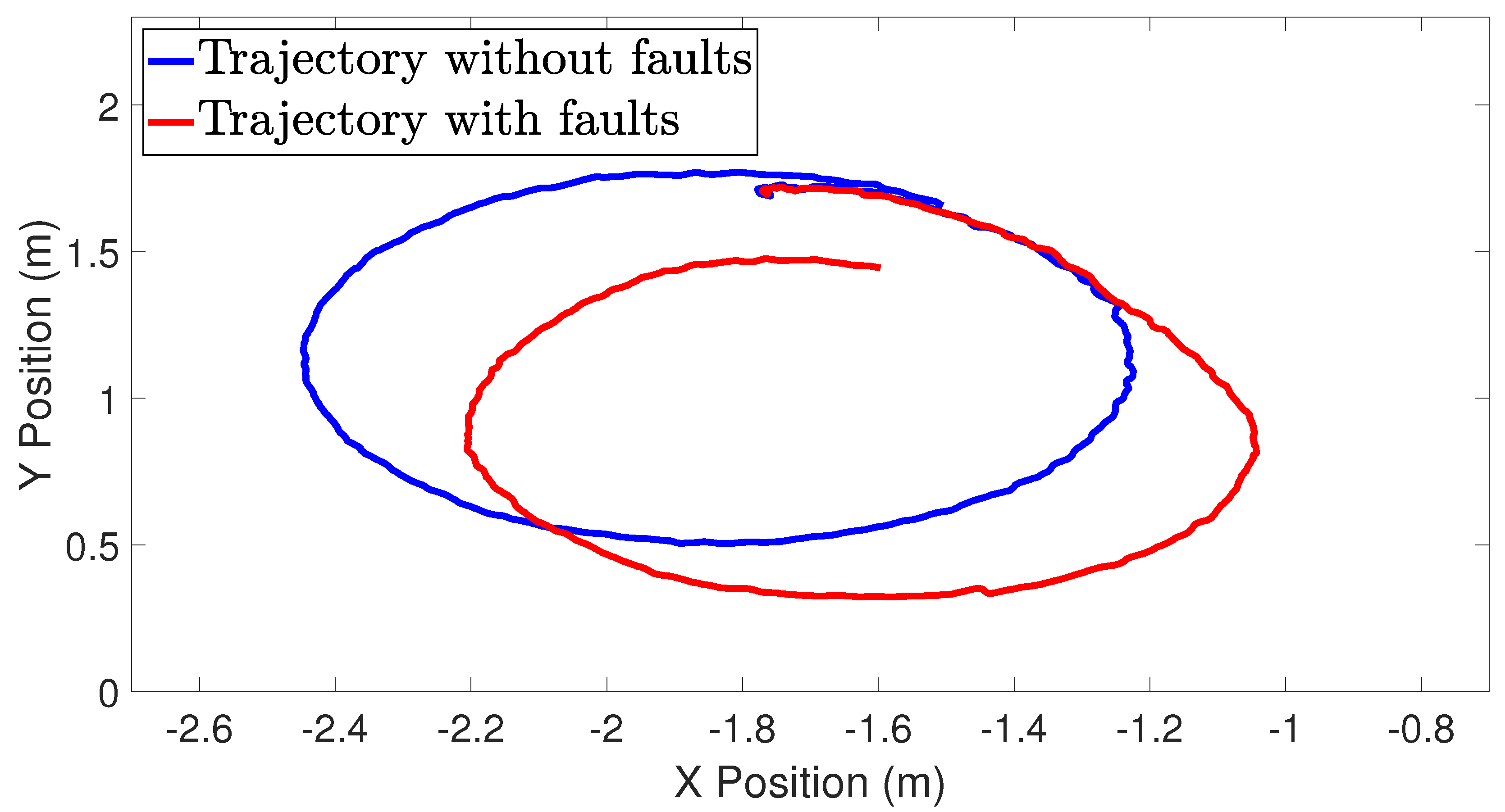
Notice that the faults and are concurrent during the interval , also and occur simultaneously during the interval . At the considered fault scenario, the faults correspond to an actuator loss of effectiveness of around 20%, 50%, and 70%. Also, the faults occur in small intervals of time such as 0.5 s. Although the system is affected by the faults during small intervals of time, Figure 4 shows that the faults cause a significant deviation from the fault-free trajectory.
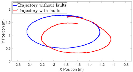
Figure 4.
Mobile robot trajectory comparison.
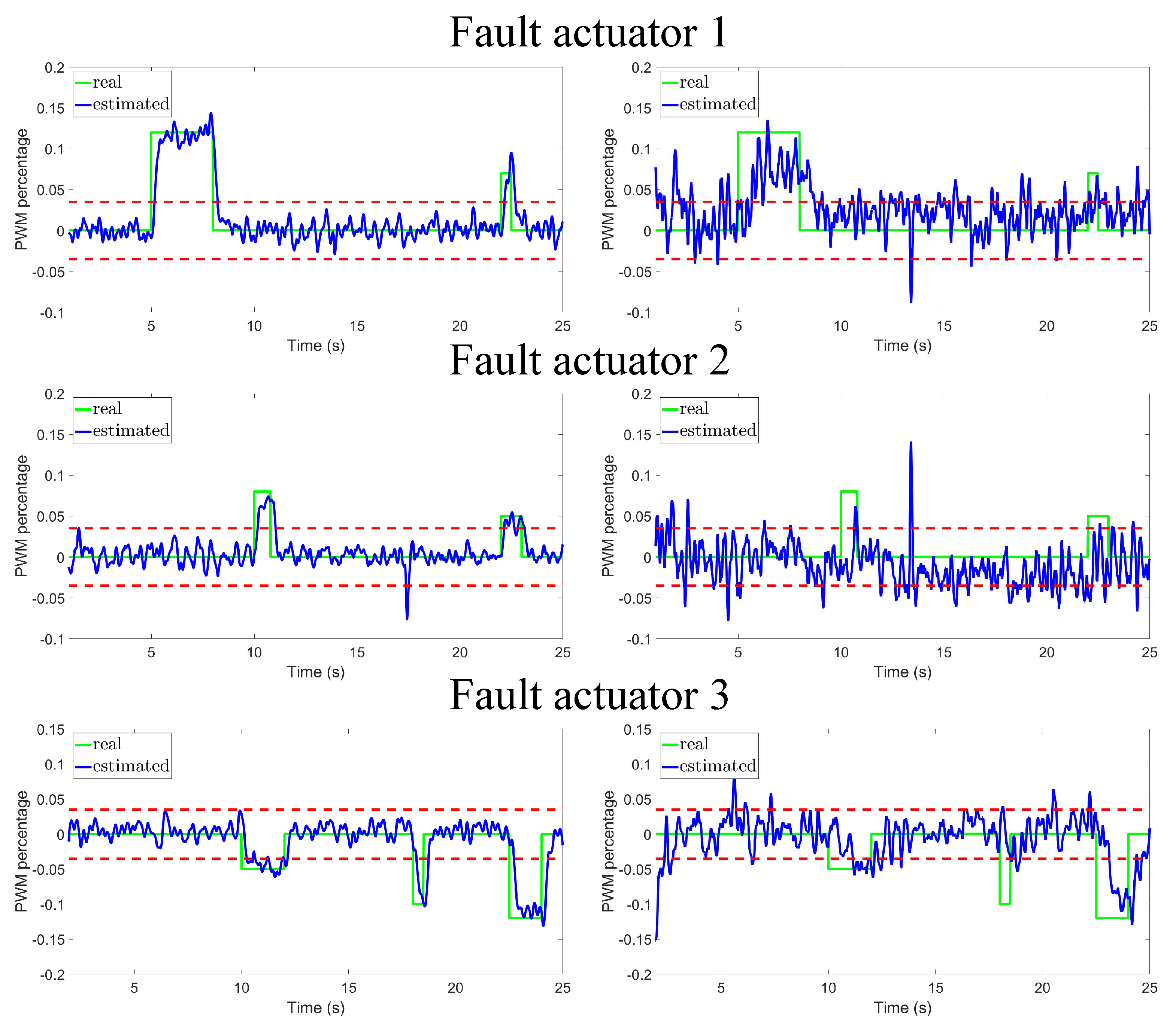
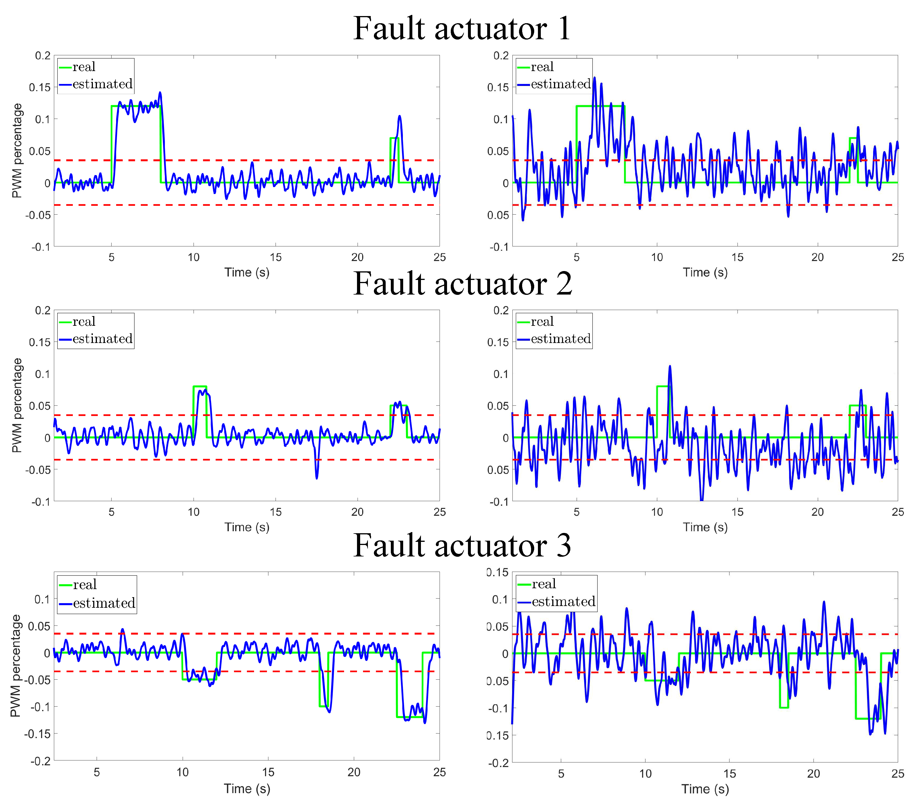
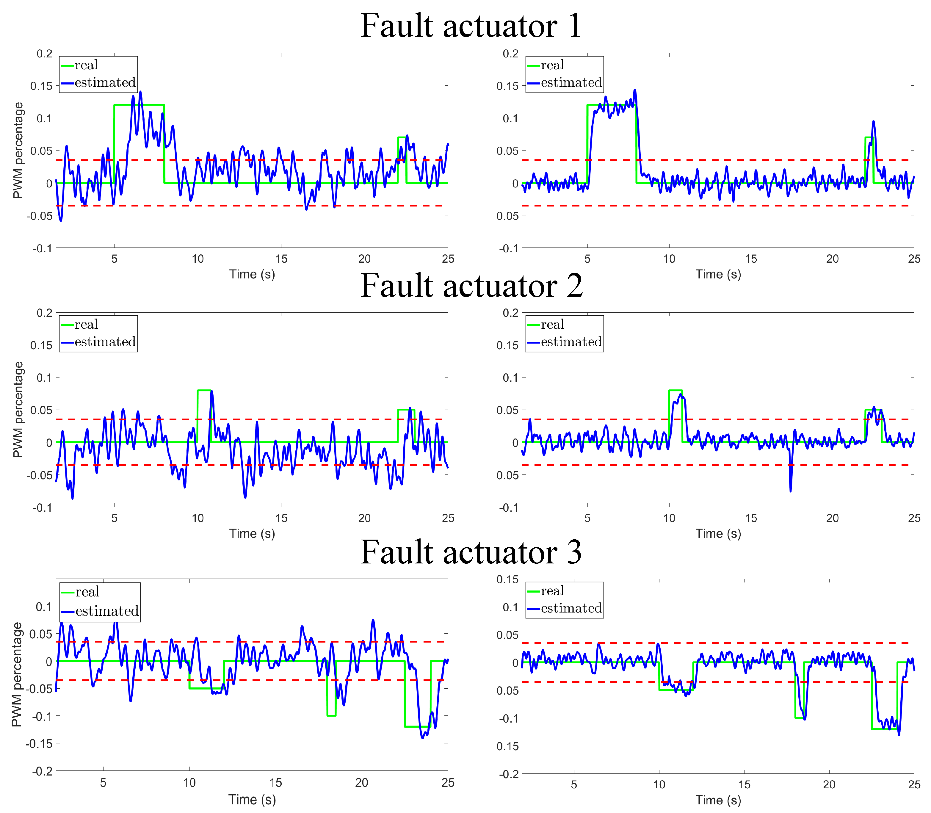
Figure 5 and Figure 6 present the fault detection using the proposed predefined-time diagnoser and the HOSM diagnoser reported in [26], respectively. In both figures, the simulations on the left correspond to the case where the proposed sensor fusion architecture is used, and on the right when it is not used. We highlight that the use of the proposed sensor fusion architecture is of major importance, in fact when this architecture is omitted, the graphics in the right columns of Figure 5 and Figure 6 show a poor performance in fault detection, exacerbating the number of false fault detections. In addition, the predefined-time diagnoser estimates faults faster than the HOSM, it also reduces false fault detections. For example, HOSM (Figure 6) detects a false fault detection in actuator 3, when the estimated fault reaches the threshold of at .
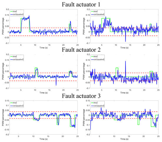
Figure 5.
The proposed diagnoser based on a predefined-time observer is used, with (left) and without (right) the proposed sensor fusion architecture.
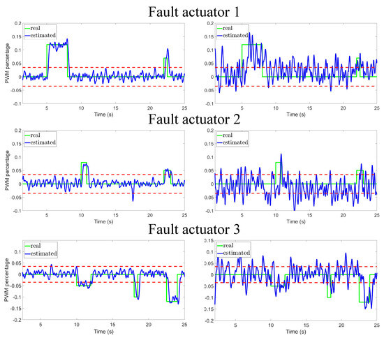
Figure 6.
A previously reported diagnoser based on an HOSM differentiator is used, with (left) and without (right) the proposed sensor fusion architecture.
Finally, Figure 7 shows that it is relevant to select the virtual sensors with the lowest variance. In fact, when is used (the one with the biggest variance), the graphics in the left column of Figure 7 show a poor performance compared with the graphics in the right column, when is used.
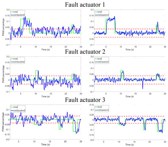
Figure 7.
Comparison of the diagnosis with (left) and (right).
Table 4 reports the RMS fault identification errors of the diagnosers when the sensor fusion architecture is applied, while Table 5 reports the RMS errors when the sensor fusion architecture is not used. From the comparison of the two tables, the proposed diagnoser architecture provides the lowest fault estimation error. Moreover, the tables show that the sensor fusion architecture reduces the fault estimation errors of the considered diagnosers.

Table 4.
Sensor fusion architecture RMS fault identification errors.

Table 5.
RMS fault identification errors when the sensor fusion architecture is not applied.
5. Conclusions
A fusion sensor architecture is introduced, comprising a homogenizer, sensor fusion stage, and voter. It has a dual purpose: generating virtual sensors comparable to the system output and providing reliable estimated signals (state and system outputs) for diagnosers, controllers, etc. To test this architecture, a case study focusing on diagnosing faults in actuators of a mobile robot was conducted, utilizing two diagnosers. In both cases, the results demonstrate that employing the proposed architecture enhances the efficiency of the diagnosis process. Specifically, false positive/negative fault detections are drastically reduced, and diagnoser convergence time is minimized.
As mentioned above, the reported diagnoser requires the input observability property from the system. Additionally, using a Kalman filter demands fast CPUs for real-time applications. In some cases, these could be considered limitations to be overcome.
In future endeavors, this architecture will be applied in various domains, including controller design, and particle filters will be considered.
Author Contributions
Conceptualization, O.B., A.L. and A.R.-T.; methodology, O.B., A.L. and A.R.-T.; software, A.L.; validation, O.B., A.L. and A.R.-T.; formal analysis, O.B., A.L. and A.R.-T.; investigation, O.B., A.L. and A.R.-T.; writing—original draft preparation, O.B., A.L. and A.R.-T.; writing—review and editing, O.B., A.L. and A.R.-T. All authors have read and agreed to the published version of the manuscript.
Funding
This research received no external funding.
Data Availability Statement
Data are contained within the article.
Conflicts of Interest
The authors declare no conflicts of interest.
References
- Flores-León, H.; Begovich, O.; Ruiz-León, J.; Ramírez-Treviño, A. Active fault detection and isolation in linear time-invariant systems: A geometric approach. Asian J. Control 2023, 25, 710–721. [Google Scholar] [CrossRef]
- Chen, J.; Patton, R.J. Robust Model-Based Fault Diagnosis for Dynamic Systems; Springer Science & Business Media: Berlin/Heidelberg, Germany, 2012; Volume 3. [Google Scholar]
- Delgado-Aguiñaga, J.; Besancon, G.; Begovich, O.; Carvajal, J. Multi-leak diagnosis in pipelines based on Extended Kalman Filter. Control Eng. Pract. 2016, 49, 139–148. [Google Scholar] [CrossRef]
- Lizarraga, A.; Begovich, O.; Ramírez, A. Real-Time Sliding Mode Fault Diagnosis for a Three-Wheeled Omnidirectional Mobile Robot. In Proceedings of the 2022 IEEE 18th International Conference on Automation Science and Engineering (CASE), Mexico City, Mexico, 20–24 August 2022; IEEE: New York, NY, USA, 2022; pp. 1953–1958. [Google Scholar]
- Gao, Z.; Cecati, C.; Ding, S.X. A survey of fault diagnosis and fault-tolerant techniques-Part I: Fault diagnosis with model-based and signal-based approaches. IEEE Trans. Ind. Electron. 2015, 62, 3757–3767. [Google Scholar] [CrossRef]
- Zhou, D.; Zhao, Y.; Wang, Z.; He, X.; Gao, M. Review on diagnosis techniques for intermittent faults in dynamic systems. IEEE Trans. Ind. Electron. 2019, 67, 2337–2347. [Google Scholar] [CrossRef]
- Delgado-Aguiñaga, J.A.; Begovich, O. Water leak diagnosis in pressurized pipelines: A real case study. In Modeling and Monitoring of Pipelines and Networks; Springer: Berlin/Heidelberg, Germany, 2017; pp. 235–262. [Google Scholar]
- Koch, W. Tracking and Sensor Data Fusion; Springer: Berlin/Heidelberg, Germany, 2016. [Google Scholar]
- Garcia-Huerta, R.A.; González-Jiménez, L.E.; Villalon-Turrubiates, I.E. Sensor Fusion Algorithm Using a Model-Based Kalman Filter for the Position and Attitude Estimation of Precision Aerial Delivery Systems. Sensors 2020, 20, 5227. [Google Scholar] [CrossRef] [PubMed]
- Bader, K.; Lussier, B.; Schön, W. A fault tolerant architecture for data fusion: A real application of Kalman filters for mobile robot localization. Robot. Auton. Syst. 2017, 88, 11–23. [Google Scholar] [CrossRef]
- Hachemi, L.; Guiatni, M.; Nemra, A. Fault diagnosis and reconfiguration for mobile robot localization based on multi-sensors data fusion. Unmanned Syst. 2022, 10, 69–91. [Google Scholar] [CrossRef]
- Ifqir, S.; Combastel, C.; Zolghadri, A.; Alcalay, G.; Goupil, P.; Merlet, S. Fault tolerant multi-sensor data fusion for autonomous navigation in future civil aviation operations. Control Eng. Pract. 2022, 123, 105132. [Google Scholar] [CrossRef]
- Abid, A.; Khan, M.T. Multi-sensor, multi-level data fusion and behavioral analysis based fault detection and isolation in mobile robots. In Proceedings of the 2017 8th IEEE Annual Information Technology, Electronics and Mobile Communication Conference (IEMCON), Vancouver, BC, USA, 3–5 October 2017; IEEE: New York, NY, USA, 2017; pp. 40–45. [Google Scholar]
- Zhang, Z.; He, X. Geometric Approach Based Fault Detection and Isolation: A Review. In Proceedings of the 2022 41st Chinese Control Conference (CCC), Hefei, China, 25–27 July 2022; IEEE: New York, NY, USA, 2022; pp. 4136–4141. [Google Scholar]
- Fridman, L.; Shtessel, Y.; Edwards, C.; Yan, X.G. Higher-order sliding-mode observer for state estimation and input reconstruction in nonlinear systems. Int. J. Robust Nonlinear Control IFAC-Affil. J. 2008, 18, 399–412. [Google Scholar] [CrossRef]
- Shtessel, Y.; Edwards, C.; Fridman, L.; Levant, A. Sliding Mode Control and Observation; Springer: Berlin/Heidelberg, Germany, 2014; Volume 10. [Google Scholar]
- Isidori, A. Nonlinear Control Systems; Springer: Berlin/Heidelberg, Germany, 1995. [Google Scholar]
- Ma, H.; Yan, L.; Xia, Y.; Fu, M. Kalman Filtering and Information Fusion; Springer: Berlin/Heidelberg, Germany, 2020. [Google Scholar]
- Gao, J.; Harris, C. Some remarks on Kalman filters for the multisensor fusion. Inf. Fusion 2002, 3, 191–201. [Google Scholar] [CrossRef]
- Hamadi, H.; Lussier, B.; Fantoni, I.; Francis, C. Data fusion fault tolerant strategy for a quadrotor UAV under sensors and software faults. ISA Trans. 2022, 29, 520–539. [Google Scholar] [CrossRef] [PubMed]
- Aldana-López, R.; Gómez-Gutiérrez, D.; Jiménez-Rodríguez, E.; Sánchez-Torres, J.D.; Defoort, M. Enhancing the settling time estimation of a class of fixed-time stable systems. Int. J. Robust Nonlinear Control 2019, 29, 4135–4148. [Google Scholar] [CrossRef]
- Trujillo, M.A.; Aldana-López, R.; Gómez-Gutiérrez, D.; Defoort, M.; Ruiz-León, J.; Becerra, H. Autonomous and non-autonomous fixed-time leader–follower consensus for second-order multi-agent systems. Nonlinear Dyn. 2020, 102, 2669–2686. [Google Scholar] [CrossRef]
- Tzafestas, S.G. Introduction to Mobile Robot Control; Elsevier: Amsterdam, The Netherlands, 2013. [Google Scholar]
- Nguyen, N.T. Model-reference adaptive control. In Model-Reference Adaptive Control; Springer: Berlin/Heidelberg, Germany, 2018; Chapter 6; pp. 126–127. [Google Scholar]
- Iqbal, M.; Bhatti, A.; Iqbal, S.; Khan, Q. Parameter estimation based fault diagnosis of uncertain nonlinear three tank system using HOSM differentiator observer. In Proceedings of the 2009 IEEE 13th International Multitopic Conference, Islamabad, Pakistan, 14–15 December 2009; IEEE: New York, NY, USA, 2009; pp. 1–6. [Google Scholar]
- Iqbal, M.; Bhatti, A.I.; Ayubi, S.I.; Khan, Q. Robust parameter estimation of nonlinear systems using sliding-mode differentiator observer. IEEE Trans. Ind. Electron. 2010, 58, 680–689. [Google Scholar] [CrossRef]
Disclaimer/Publisher’s Note: The statements, opinions and data contained in all publications are solely those of the individual author(s) and contributor(s) and not of MDPI and/or the editor(s). MDPI and/or the editor(s) disclaim responsibility for any injury to people or property resulting from any ideas, methods, instructions or products referred to in the content. |
© 2024 by the authors. Licensee MDPI, Basel, Switzerland. This article is an open access article distributed under the terms and conditions of the Creative Commons Attribution (CC BY) license (https://creativecommons.org/licenses/by/4.0/).


