A Sparsity-Invariant Model via Unifying Depth Prediction and Completion

Abstract

The development of a sparse-invariant depth completion model capable of handling varying levels of input depth sparsity is highly desirable in real-world applications. However, existing sparse-invariant models tend to degrade when the input depth points are extremely sparse. In this paper, we propose a new model that combines the advantageous designs of depth completion and monocular depth estimation tasks to achieve sparse invariance. Specifically, we construct a dual-branch architecture with one branch dedicated to depth prediction and the other to depth completion. Additionally, we integrate the multi-scale local planar module in the decoders of both branches. Experimental results on the NYU Depth V2 benchmark and the OPPO prototype dataset equipped with the Spot-iToF316 sensor demonstrate that our model achieves reliable results even in cases with irregularly distributed, limited or absent depth information.

1. Introduction

Dense depth maps play an important role in a wide range of vision applications, such as autonomous driving, scene reconstruction, and augmented reality. However, despite the advancements in range-sensing techniques, depth information acquired from sensors like Time of Flight (ToF) cameras or Light Detection and Ranging (LiDAR) sensors often suffers from low-resolution or sparsity issues. Consequently, guided depth completion methods are widely employed to improve the quality and resolution of the depth maps.

The guided depth completion task aims to utilize color images as guidance to complete sparse depth maps obtained from depth sensors. The acquisition of color images has become more reliable with the continuous advancement of camera technology, and the image augmentation used during the training process can also effectively handle basic changes, such as lighting, common environments, and camera adjustments. However, the acquisition of sparse depth maps is affected by various factors such as depth sensor hardware configuration and environmental conditions, resulting in significant changes in the distribution of effective depth value points in the depth map.

Firstly, the different working principles of sensors will lead to differences in the data distribution of the sparse depth maps. Secondly, even for the same type of sensor, the sparsity of depth maps acquired under different configurations may vary. Additionally, some light reflection-based depth sensors are greatly influenced by factors such as environmental lighting, depth range, and object reflectivity, which may result in invalid depth points at different positions in the depth map, forming black hole areas. If sensor malfunction or other unforeseen circumstances occur, it may lead to extremely sparse depth maps or even an absence of depth points. Considering these, in this paper, we focus on improving the generalization ability of the model on sparse depth maps with various distribution patterns and different sparsity levels and ensuring reliable depth prediction even when the input depth information is limited or completely absent in real-world applications.

To date, various methods have been proposed for color-guided depth completion tasks, including models with complex network structures [1,2,3,4], models with spatial propagation networks [5,6,7,8,9,10], models based on three-dimensional structure design [11,12,13,14] and the latest model based on transformer [15,16,17]. However, most of these models do not fully consider the generalization capability of models across different sparse depth maps, making them sensitive to the differences in sparse depth maps. Although some researchers have explored the generalization of models, the number of related studies is still relatively limited. Some of them utilize sparse convolution [18] and sparsity-aware augmentation [19,20] to handle sparse inputs. Others employ non-learning methods to complete the sparse depth map, which is followed by optimization using color images [21,22,23]. Additionally, some utilize depth maps obtained from pre-trained monocular depth estimation networks as depth priors input to the network [19,24]. While these methods focus on addressing variations in sparsity levels, their performance still deteriorates significantly in cases of extremely sparse depth points and no depth points.

It is observed that when the input depth map provides a sufficient number of valid points, the accuracy of the depth map generated by depth completion surpasses that of the monocular depth estimation task. Meanwhile, when the input depth map is extremely sparse or completely missing, the depth completion task turns into a monocular depth estimation problem. In this case, models specifically designed for monocular depth estimation outperform the depth completion models. Inspired by this, we consider adopting the design ideas from the monocular depth estimation task to improve the depth prediction ability of the depth completion model when the depth map is extremely sparse or completely absent.

Monocular depth estimation generates a dense depth map from a single color image. Two-dimensional color images, unlike sparse depth maps, cannot directly present three-dimensional information. Therefore, most methods in this field focus on leveraging geometric priors to improve depth prediction results. Scene plane and surface normal vectors are closely related to depth values, so they are often embedded into the model architecture as representations of scene structure information or introduced into the loss function for training. Following the local planar assumption, methods [25,26,27,28,29,30] utilize surface normal as an intermediate representation to enforce constraints on local 3D points belonging to the same plane, ensuring that the vectors formed by any two pixels within a plane are perpendicular to the surface normal. Yin et al. [31,32] introduced the concept of virtual normal, extending the constraint range from a local window to the entire global image. GeDepth [33] also approaches the problem from the perspective of a global scene structure. It introduces a novel ground-embedding module to decouple camera parameters from pictorial cues, thereby enhancing generalization. There are also some methods [30,34] that directly predict plane coefficients for local patches to guide the final depth prediction based on the conversion relationship between these coefficients and depth values, showing promising results.

The complementary strengths of the completion methods, which excel in scenarios with sufficient depth information, and prediction methods, which are adept at handling no depth input, inspire us to unify the advantageous designs of both tasks. Although numerous methods have been developed for depth completion or depth prediction individually, these two research lines have progressed almost independently. To leverage their advantageous designs, in this work, we build our model upon a dual-branch encoder–decoder architecture that has been proven effective in depth completion tasks [4,35,36]. Additionally, we introduce some scene structure-related designs, such as plane representation and surface normal, which have been validated as effective in monocular depth estimation tasks, into both the model architecture and loss functions.

Specifically, we designed a dual-branch network architecture. One branch takes the color image as input and focuses on the depth prediction task, while the other branch simultaneously processes the color image and depth information for the depth completion task. Both branches incorporate a local plane constraint module in their decoders to ensure high-quality depth estimation when depth points are sparse or absent. This module predicts plane coefficients using feature maps at multiple scales in the decoder and ensures the consistency of plane coefficients within local regions as the feature map scales are progressively recovered. In addition, a surface normal-based loss function is also adopted to enforce geometric constraints on the model’s predicted depth maps.

By integrating the dual-branch encoder–decoder architecture with the local planar guidance module, together with a mixture training strategy that utilizes data with different levels of sparsity for training, our model exhibits remarkable generalization capabilities for both depth completion and depth prediction tasks. It consistently achieves high performance across a wide range of input depth sparsity levels. Experimental results on the NYU Depth V2 dataset [37] showcase the superiority of our approach compared to recent sparse-invariant methods [38], particularly when dealing with extremely sparse or absent input depth. Furthermore, to validate the reliability of the model in real-world applications, we utilized an OPPO prototype equipped with an iTOF depth sensor to collect a dataset in indoor environments for testing. The results demonstrate that our model can effectively handle sparse depth maps with noise and irregular distributions encountered in practical applications.

The main contributions of the work in this paper are summarized as follows:

• We designed a depth completion model with high generalization capability, which effectively handles sparse depth maps with different sparse levels and irregular distribution, and ensures reliable depth prediction even when the input depth is limited or completely absent.
• We integrated effective designs from both depth completion and monocular depth estimation tasks, establishing a dual-branch structured model. A multi-scale local plane constraint module and a surface normal-based loss function are adopted to further exploit scene structure-related information.
• Our model achieves reliable depth results even when depth information is limited or completely absent, as demonstrated on the benchmark dataset NYU Depth V2 [37]. In real-world applications, this model can also effectively handle sparse depth maps with noise and irregular distribution.

2. Related Work

2.1. Monocular Depth Estimation

The monocular depth estimation task infers the corresponding depth map from a single color image. Due to the absence of spatial information and depth scale from sparse depth points, most monocular depth estimation methods focus on exploring the geometric relationships in the scene.

Some works [27,28,29] utilize the geometric constraint that “the surface composed of any three points in the plane should be perpendicular to the surface normal vector of this plane” to design corresponding network architectures and loss functions. Structdepth [28] introduces Manhattan normal constraints and coplanarity constraints. The Manhattan normal constraint aligns major surfaces, such as floors, ceilings, and walls, with dominant directions. The coplanarity constraint enforces coplanarity among a set of three-dimensional points within the same planar region. Long et al. [29] propose an adaptive surface normal constraint method. They first randomly sample a set of three-dimensional points on a specified plane to determine the local plane and then derive the constraint relationship between the plane and the surface normals. Yin et al. [31,32] introduce global geometric constraints based on “virtual normal” to address the generalization problem of monocular depth estimation. Virtual normal refers to the normal determined by a pseudo-plane formed by randomly sampling three points from three-dimensional space. Geometric constraint losses between predicted and ground truth values are utilized to enhance the accuracy and robustness of monocular depth estimation.

In addition to adjusting the loss functions, some models directly incorporate plane constraints into their network. Among them, Geonet [25] and Geonet++ [26] simultaneously predict the depth and surface normal from a single image. They employ one network to convert depth into surface normal and another network to convert surface normal into depth, thereby enforcing geometric consistency and accuracy between the two outputs. Such a design constrains the network to achieve high consistency and accuracy between the two outputs. In the studies by Lee et al. [30] and Patil et al. [34], depth is not directly predicted. Instead, based on the conversion relationship between the depth and surface normal vector, plane coefficients are first predicted and then converted into a depth map. By constraining regions with consistent plane coefficients, the consistency of local planes is achieved.

We know that monocular depth estimation suffers from the issue of scale ambiguity; thus, it usually did not directly take l1 or l2 as loss to supervise the network. Lee et al. [39] proposed an algorithm to combine multiple loss terms adaptively for training a monocular depth estimator. The most commonly used loss in this task for direct depth supervision is scale-invariant loss [40] due to its scale invariance. This loss emphasizes the relative relationships between pixels in the depth map, considering the relationships between pixel pairs as the criterion, comparing the consistency between the depth differences of pixel pairs in the predicted result and those in the corresponding pixel pairs in the ground truth depth map. By optimizing this loss function, the influence of absolute global scale on the results is mitigated.

Fu et al. [41] discretized continuous depth into a series of intervals and transformed the depth estimation into a classification problem. Then, they designed a strategy with gradually increasing intervals to discretize the depth values. AdaBins [42] divides the depth range into different intervals based on the characteristics of each image, enabling the network to adaptively focus on regions with varying depths. Its main contribution lies in a Mini-ViT module which uses global information to compute the width of each depth interval as well as the probability values of the depth intervals. In this way, the method is able to generate smoother depth maps. Similarly, PixelFormer [43] utilizes the transformer structure to formulate the prediction problem as ordinal regression over depth bin centers, with a Bin Center Predictor module predicting bins at the coarsest level using pixel queries.

2.2. Image-Guided Depth Completion

Image-guided depth completion has been widely studied these years, while the model structure and the modality fusion are also becoming diverse and complex. In Figure 1, we illustrate the evolution of network structures for the guided depth completion task.

Single Enc–Single Dec Ma et al. [2] first employed a single encoder–single decoder architecture, utilizing color images to guide the completion of incomplete depth maps. Later methods [44,45] made individual enhancements in their respective decoders. Instead of direct fusion, some approaches [46,47,48] use two separate convolution units to extract features from color images and depth map inputs independently. After concatenating the multi-modal features at the feature level, they are fed into subsequent encoder–decoder networks to regress the complete depth map, completing the pixel-wise prediction task.

Dual Enc–Single Dec Approaches based on dual encoder–single decoder architecture [20,49,50,51,52,53] adopt the divide-and-conquer strategy, utilizing separate encoders for color images and depth maps to handle the two modalities independently and extract corresponding features. These features are fused into a correlated feature representation and passed to the decoder for further processing. The features acquired by the two encoders for their respective modalities typically exhibit consistent scales, easing their fusion in the decoder through concatenation, addition, or alternative methods. While the aforementioned methods solely integrate the features of color images and depth maps at a single spatial scale, multiple studies [54,55,56,57] achieve multi-scale feature fusion. They leverage deep low-resolution features to capture global information and fully utilize shallow high-resolution features to prevent the loss of local structural information, which is crucial for dense prediction tasks.

Dual Enc–Dual Dec The dual encoder–dual decoder structure [1,58,59] adds an additional decoder compared to the single decoder structure, as shown in Figure 1. In this architecture, two encoder–decoder networks receive images and sparse depth as inputs, respectively. The fusion operation for dual encoder–single decoder networks typically occurs between these two encoders. However, for dual encoder–dual decoder networks, high-resolution features obtained from the image encoder–decoder network are used to guide the depth recovery process of the sparse depth decoder. The fusion between the decoder and depth encoder also typically occurs at multiple scales.

Dual-Branch The core design of a dual-branch structure is to predict depth maps from two complementary perspectives and then adaptively fuse the predictions of the two branches. Van et al. [36] introduced the first dual-branch model from both global and local perspectives, yielding favorable results. As the network evolves, the two-branch model with rgb and surface normal branches [4], or with image dominant and depth dominant branches [35], are gradually proposed.

Two-Stage A two-stage structure [60,61,62,63] generally adopt a coarse-to-fine prediction strategy. Inspired by the residual learning framework, some two-stage works [64,65,66,67] decompose the final depth prediction into the estimation of a dense depth map and a residual depth map. These two maps are then linearly combined to obtain the final depth result. Additionally, there are coarse-to-fine structures incorporating the depth refinement module, the spatial propagation network, after Cheng et al. [68] first proposed a convolutional spatial propagation network used for depth completion, which generates a spatial-invariant affinity matrix to refine depth. Following this idea, some methods [5,6,7,8,10,35] continuously advanced it by continuously expanding the field of propagation or iterative propagation strategy.

Depth encodes three-dimensional information in the scene. Therefore, in addition to standard convolution, methods such as sparse-conv [18], norm-conv [21,22], and various 3D convolutions [11,69], as well as graph-conv-based approaches [70,71], are applied in this task. Additionally, physical quantities representing three-dimensional scene information, such as surface normals [4,72] and twin-surface representations [3], also serve as auxiliary information to help network training.

2.3. Sparsity-Invariant Depth Completion

Early works designed some sparsity-aware convolutions like sparse convolution [18] and normalized convolution [21,22]. Xiong et al. [70] considered different sparse patterns and proposed an end-to-end network with a graph convolution module, which effectively utilized the relationships between 3D points and their neighborhoods. In experiments, they compared four quasi-random sampling strategies against random sampling, verifying its generalization ability in indoor scene depth completion.

Some studies [19,23,24] utilize pre-trained monocular depth estimation networks to address sparse generalization issues. Long et al. [24] consider different sensor configurations and decompose the depth completion into two subtasks: relative depth map estimation and scale recovery. The model first estimates a relative depth map from a single color image and then incorporates sparse depth as scale information to obtain the final depth map. Yin et al. [19] directly utilize depth map priors obtained from pre-trained monocular depth estimation models trained on large-scale datasets for individual color images. Subsequently, this prior is used as input for completing sparse, semi-dense, or noisy depth maps obtained from various depth sensors or multi-view reconstruction algorithms. They also simulate various sparse patterns in the training data for network training. Wang et al. [23] propose a plug-and-play module. Given a pre-trained depth prediction model, the module can accept depth maps under arbitrary sparse patterns as input. By iteratively updating intermediate feature maps in the pre-trained depth estimation model, the method ensures consistency between the model output and the given sparse depth, thereby improving the final depth prediction results.

Differently, Conti et al. [38] did not choose to directly feed sparse depth points to convolutional layers but rather iteratively merge the sparse input points with multiple depth maps predicted by the network to handle highly variable data sparsity. In addition, Yin et al. [19] leverage diverse data augmentation to improve the model’s generalization to different data domains and noise. Ryu et al. [20] simultaneously use sparse depth maps with various lidar scan-lines as input during training, and they proposed a consistency loss between them to obtain a scan-line resolution-invariant depth completion model. G2-MonoDepth [73] introduced a novel unified loss to handle varying depth sparsity in input raw data and diverse scales of output scenes. Additionally, it employed a data augmentation pipeline to simulate various real-world artifacts in raw depth maps for training.

3. Preliminary: Pseudo-Plane Coefficients

Given a depth map and camera intrinsic parameters, we can use the pinhole camera model to back-project each pixel into 3D space. Assuming the focal lengths $f_x$ and $f_y$, and the principal point $(u_0, v_0)$, each pixel $p=(u, v)$ can be mapped to a 3D point P as follows:

$$Z=D(u, v),\hspace{1em}X=\frac{Z(u-u_0)}{f_x},\hspace{1em}Y=\frac{Z(v-v_0)}{f_y}$$

(1)

where $D(u, v)$ represents the depth value at pixel $(u, v)$.

Assuming $P={(X, Y, Z)}^T$ are the three-dimensional coordinates of a point, the point-normal equation of the tangent plane at point P can be written as

$$\overrightarrow{n}·P+d=0$$

(2)

where $\overrightarrow{n}={(a, b, c)}^T$ is the normal vector to the plane, and $-d$ is the distance from the origin to the plane. Substituting P from Equation (1) into Equation (2), we obtain the following equation:

$$\frac{1}{Z}=\frac{-a}{f_{x}d}u+\frac{-b}{f_{y}d}v+\frac{1}{d}(\frac{a}{f_x}{u}_0+\frac{b}{f_y}{v}_0-c)$$

(3)

Assume that

$$\begin{array}{cc}\hfill {\alpha }^{\prime }& =\frac{-a}{f_{x}d}\hfill \\ \hfill {\beta }^{\prime }& =\frac{-b}{f_{y}d}\hfill \\ \hfill {\gamma }^{\prime }& =\frac{1}{d}(\frac{a}{f_x}{u}_0+\frac{b}{f_y}{v}_0-c)\hfill \\ \hfill \rho & =\sqrt{{\left({\alpha }^{\prime }\right)}^2+{\left({\beta }^{\prime }\right)}^2+{\left({\gamma }^{\prime }\right)}^2}\hfill \end{array}$$

(4)

Then, we normalize these three values, ${\alpha }^{\prime },{\beta }^{\prime },{\gamma }^{\prime }$, to obtain

$$\begin{array}{cccc}\hfill \alpha & =\frac{{\alpha }^{\prime }}{\rho },\hspace{1em}\beta \hfill & \hfill =\frac{{\beta }^{\prime }}{\rho },\hspace{1em}\gamma & =\frac{{\gamma }^{\prime }}{\rho }.\hfill \end{array}$$

(5)

Therefore, the above Equation (3) can be simplified to the following Equation (6):

$$Z={\left[(\alpha u+\beta v+\gamma )\rho \right]}^{-1}$$

(6)

In this way we encoded the camera intrinsic parameters and the three-dimensional plane into the plane coefficients $C=(\alpha , \beta , \gamma , \rho )$ and refer to them as pseudo-plane coefficients.

In the following proposed modules, we first predict the pseudo-plane coefficient for each pixel. Subsequently, we use Equation (6) to calculate the specific depth values based on the two-dimensional coordinates of each pixels. The pseudo-plane coefficient not only significantly reduces calculation complexity but also reduces the model’s dependency on camera parameters.

4. The Proposed Method

Figure 2 presents an overview of our proposed method. It combines a dual-branch encoder–decoder architecture with a multi-scale local planar guidance module (MLPGM) to create a unified model capable of handling both depth prediction and depth completion tasks. More specifically, we construct dual-branch encoder–decoders with one branch dedicated to depth prediction (DP) and the other focused on depth completion (DC). In the decoder of each branch, a multi-scale local planar guidance module is integrated to ensure high-quality results when the input depth is extremely sparse or missing. The details of each module will be introduced in the following sections.

4.1. Dual-Branch Encoder–Decoder Architecture

Dual-branch encoder–decoder architectures have been employed in previous depth completion methods [4,35,36], yielding promising results. Additionally, Hu [74] observe that when employing a mixed training strategy, the dual-branch architecture exhibits greater invariance to different sparsity levels compared to a single-branch model regardless of whether the latter incorporates sparse-invariant convolutions or not. Therefore, we adopt this dual-branch architecture to achieve better sparse invariance.

In the first branch, we take a single color image as input and focus on predicting depth when no input depth information is available. This prediction branch consists of a ResNet101-based encoder [75] and a decoder composed of five up-convolution blocks. Each up-convolution block comprises an upsampling layer, a convolutional layer, a batch normalization (BN) layer, a ReLU activation layer, and a Resblock. These blocks are denoted as the “F” or “U” blocks in Figure 2. Skip connections are utilized to merge the features from each encoder layer with those of the corresponding decoder blocks. Additionally, between the second and third decoder blocks, a dynamic atrous spatial pyramid pooling (DASPP) module [76] is inserted on the $\frac{1}{8}$ scale features to capture more contextual information.

In the second branch, we take a sparse depth map, together with the final feature map generated by the prediction branch “(f)”, as inputs. The two inputs are fed through a convolution layer individually and then concatenated together, as illustrated by the “P” block in Figure 2. In this completion branch, a shallower encoder structure is adopted, which only utilizes two Resblocks at each scale, to handle sparse depth information. At each scale, the features extracted from the first branch are also fused to the second branch through the “R” block, which comprises a convolution layer, BN, and ReLU to leverage color information better. The decoder shares the same structure as the one in the first stream.

4.2. Multi-Scale Local Planar Guidance Module

Introducing scene structure information into the network structure to improve the prediction quality of the depth map has been widely adopted in the monocular depth estimation task [30,34]. In this paper, we introduce a plane-based design aimed at handling the extreme case: that is, ensuring the depth prediction accuracy when there is no sparse depth point input. Thus, based on the local plane assumption, we introduce multi-scale local planar guidance modules in both branches to ensure accurate and smooth depth variations for points on the same plane as the decoder scales progressively recover.

From the $\frac{1}{8}$ scale, the MLPGM starts predicting the plane coefficients $(\alpha ,\beta ,\gamma ,\rho )$ of the local plane at each scale. The predicted coefficients are then used to compute depth values according to Equation (6). By capturing the local planar structures, the MLPGM can generate more accurate depth maps compared to directly predicting depth values at a lower resolution and upsampling them to the full resolution. As illustrated in Figure 2, the MLPGM is integrated into multiple scales of both decoders.

Unlike previous methods that only use the local planar guidance (LPG) to guide full-resolution depth estimation [30,34], we extend its usage by employing it to generate a depth map with double the resolution of the input feature maps, as shown in the “LPG” block in Figure 2. We then fuse these higher-resolution depth maps with the corresponding decoder features to guide the features at the next scale.

At a single scale, the specific operations within an LPG can be understood from the LPG module shown in Figure 2. We take the $1/s$ scale as an example to illustrate the specific steps of LPG. Firstly, the feature $f^{1/s}$ passes through a convolution layer with an output feature layer of 4, yielding pseudo-plane coefficients $planecoe{f}^{1/s}$. Then, it is split into two parts. One portion is initially upsampled to the $2/s$ scale, where the depth map is computed using Equation (6). Subsequently, it is combined with the features of the subsequent scale and fed into the network. The other part is directly upsampled to the full resolution scale $s/s$. After conversion to a depth map, it is concatenated with the full-resolution depth maps outputted by LPG at other scales, as well as the features of the last layer at full resolution, and finally passed through module R to obtain the final depth map output. During the upsampling process of the LPG module, we utilize the nearest-neighbor upsampling method for plane coefficients to maintain consistency with the local plane assumption and ensure that the upsampled pixels remain within the same plane. The upsampling process is illustrated in Figure 3.

4.3. Training Loss

We use the widely used scale-invariant loss (SIL) $L_{SIL}$ [40] in conjunction with a mean normal loss (MNL) $L_{MNL}$ [34] and a gradient loss (GL) $L_{GL}$ for training. Each of these losses is defined as follows.

4.3.1. Scale-Invariant Loss

The scale-invariant loss [40] measures the relationships between points regardless of the absolute global scale. Hence, in the monocular depth estimation tasks [30,34,39] where inherent scale ambiguity exists, this type of loss function is widely employed. In our work, we employ it to ensure reliable results when the input depth is extremely sparse or absent. The scale-invariant loss is defined by

$$L_{SIL}=\frac{1}{n}\sum _i{g}_i^2-\lambda \frac{1}{n^2}{\left(\sum _i{g}_i\right)}^2,$$

(7)

where $g_i=log{z}_i-log{z}_i^{*}$, $z_i$ is an estimated depth value at pixel i, $z_i^{*}$ is the ground truth, and n is the pixel number.

4.3.2. Mean Normal Loss

The mean normal loss [34] measures the disparity between the estimated normal of a pixel, which is determined by considering its neighboring pixels, and the ground truth normal of that pixel.

We depict the process of inferring surface normal from the depth map as a least-squares problem. Specifically, for any pixel i, assuming its depth is $z_i$, we first compute its three-dimensional coordinates $(x_i, y_i, z_i)$ from its two-dimensional coordinates $(u_i, v_i)$ based on the pinhole camera model, as described by Equation (1). Then, to compute the surface normal of pixel i, we first determine the tangent plane passing through pixel i in 3D space. We proceed with the assumption that pixels within the local neighborhood of pixel i lie on the same tangent plane. Specifically, we define the set of neighboring pixels ${\mathcal{N}}_i$, including pixel i itself.

With these pixels lying on the tangent plane, the estimated surface normal vector $\overrightarrow{n}=(n_x, n_y, n_z)$ should satisfy the following equation:

$$A\overrightarrow{n}=\overrightarrow{b},\hspace{1em}subject to {\left|\right|\overrightarrow{n}\left|\right|}_2^2=1$$

(8)

where A is the data matrix formed by stacking the 3D points within the patch as shown in Equation (9).

$$A=\left[\begin{array}{ccc}{x}_1& y_1& z_1\\ x_2& y_2& z_2\\ ⋮& ⋮& ⋮\\ x_K& y_K& z_K\end{array}\right]\in {\mathcal{R}}^{K\times 3}$$

(9)

$\overrightarrow{b}\in {\mathcal{R}}^{k\times 1}$ is a constant vector consisting of all ones. K is the size of $\mathcal{N}i$. The least-squares solution to this problem, i.e., minimizing $\left|\right|A\overrightarrow{n}-\overrightarrow{b}{\left|\right|}^2$, has a closed-form solution. Thus, we can obtain

$$\overrightarrow{n}=\frac{{\left(A^{T}A\right)}^{-1}{A}^T\overrightarrow{b}}{\parallel {\left(A^{T}A\right)}^{-1}{A}^T\overrightarrow{b}{\parallel }_2}.$$

(10)

In this loss function, to estimate the normal vector $\overrightarrow{n}$, we construct a matrix A by stacking the 3D points within a $k\times k$ patch centered around the pixel from $\mathcal{N}i$ and solve the equation $A\overrightarrow{n}=\overrightarrow{b}$. To compute the mean normal loss, we first estimate surface normal vectors for all K non-overlapping patches in the predicted depth map Z and the ground truth depth map $Z^{*}$, and then we calculate the loss by penalizing their differences. Therefore, the mean normal loss is defined as

$$L_{MNL}=\sum _i{\parallel \overrightarrow{n_i}-{\overrightarrow{n_i}}^{*}\parallel }_1,$$

(11)

where $\overrightarrow{n_i}$ is the normal vector calculated from the predicted depth map, and ${\overrightarrow{n_i}}^{*}$ is the normal vector computed from the ground truth depth map. The difference between the two vectors is measured by subtraction.

As the value of K increases, the selected patch may no longer satisfy the plane assumption due to depth discontinuities within the patch. Even in such cases, the mean normal loss still provides an effective supervision, because it penalizes inconsistencies between the local tangent plane within the patch and $n_i$. According to Equation (10), we can also observe that the loss directly influences the depth of all points within the patch through A.

4.3.3. Gradient Loss

The gradient loss calculates the discrepancy between the gradients computed from the predicted depth map and the ground-truth depth map, helping to achieve smoother planes and sharper edges. It is defined by

$$L_{GL}=\left|\right|G-G^{*}{\left|\right|}_1,$$

(12)

where G and $G^{*}$ represent the gradient maps of the prediction and ground truth, respectively.

4.3.4. Overall Loss Function

We constrain the results of both the prediction branch and the completion branch in the network structure to ensure that the dense depth maps they generate can complement and assist each other. For the depth maps predicted separately by the two branches, the loss functions are defined as follows:

$$\begin{array}{cc}\hfill L_{DP}& =L_{SIL}+L_{MNL}+L_{GL}\hfill \\ \hfill L_{DC}& =L_{SIL}+L_{MNL}+L_{GL}\hfill \end{array}$$

(13)

The overall loss function of the entire network is defined as

$$L=L_{DP}+w{L}_{DC}$$

(14)

Here, w represents the corresponding weight of the depth map in the depth prediction branch.

5. Experiment

5.1. Experimental Setup

We first evaluate the proposed method on the NYU Depth V2 benchmark dataset [37], which contains 464 indoor scenes captured by a Kinect camera. We follow the official train/test split, using 249 scenes for training (∼50 K images) and 215 scenes (654 images) for testing. Each image is downsampled to $320\times 240$ and subsequently center cropped to $304\times 228$. For performance evaluation, we only show the most primary evaluation metrics, root mean square error (RMSE), to showcase the results for clear comparison. Based on the predicted depth map Z and the ground truth depth map $Z^{*}$, the calculation formula for RMSE is as follows, where N represents the number of valid pixels in $Z^{*}$.

$$RMSE=\sqrt{\frac{1}{N}{\sum }_{i=1}^N{(Z-Z^{*})}^2}$$

(15)

The proposed method is implemented using the PyTorch framework [77] and trained on a single NVIDIA GTX 2080Ti GPU. During training, we employ the AdamW optimizer [78] with $\beta 1=0.9$ and $\beta 2=0.999$. We train the model for a total of 30 epochs, about nearly 100,000 iterations, with a batch size of 16. The learning rate is scheduled using polynomial decay, starting from a base learning rate of ${10}^{-3}$ with a power of $p=0.9$, as seen in Figure 4a. The parameter w in the overall loss function is set as follows, assuming the total number of iterations is T, and the current iteration is t. When t < 0.25 T, w = 1; when t < 0.5 T, w = 0.5; when t < 0.5 T, w = 0.25; and when t < 0.75 T, w = 0.1. Figure 4b shows the overall loss curve of the model. From the figure, it can be seen that there is a significant drop in the loss curve at the corresponding iterations. Additionally, the loss function steadily decreases from the beginning of the training. Although the rate of decrease changes in the mid to late stages of training, it still shows a slow convergence to stability.

In addition, we adopt a mixture strategy that involves training with data of different sparsity levels. Specifically, we randomly sample 5, 50, 100, 200, or 500 sparse depth points from the ground truth maps. Approximately 50% of the depth maps contain 500 depth points, while the remaining 50% consist of varying sparsity levels. This strategy allows the model to learn from a diverse range of sparse depth inputs. Furthermore, we augment the training data by applying random horizontal flipping to both the images and the paired sparse depth maps. We also introduce random contrast, brightness, and color adjustments within a range of $[0.9,1.1]$ to the color images and utilized the CutDepth method [79] to augment depth maps.

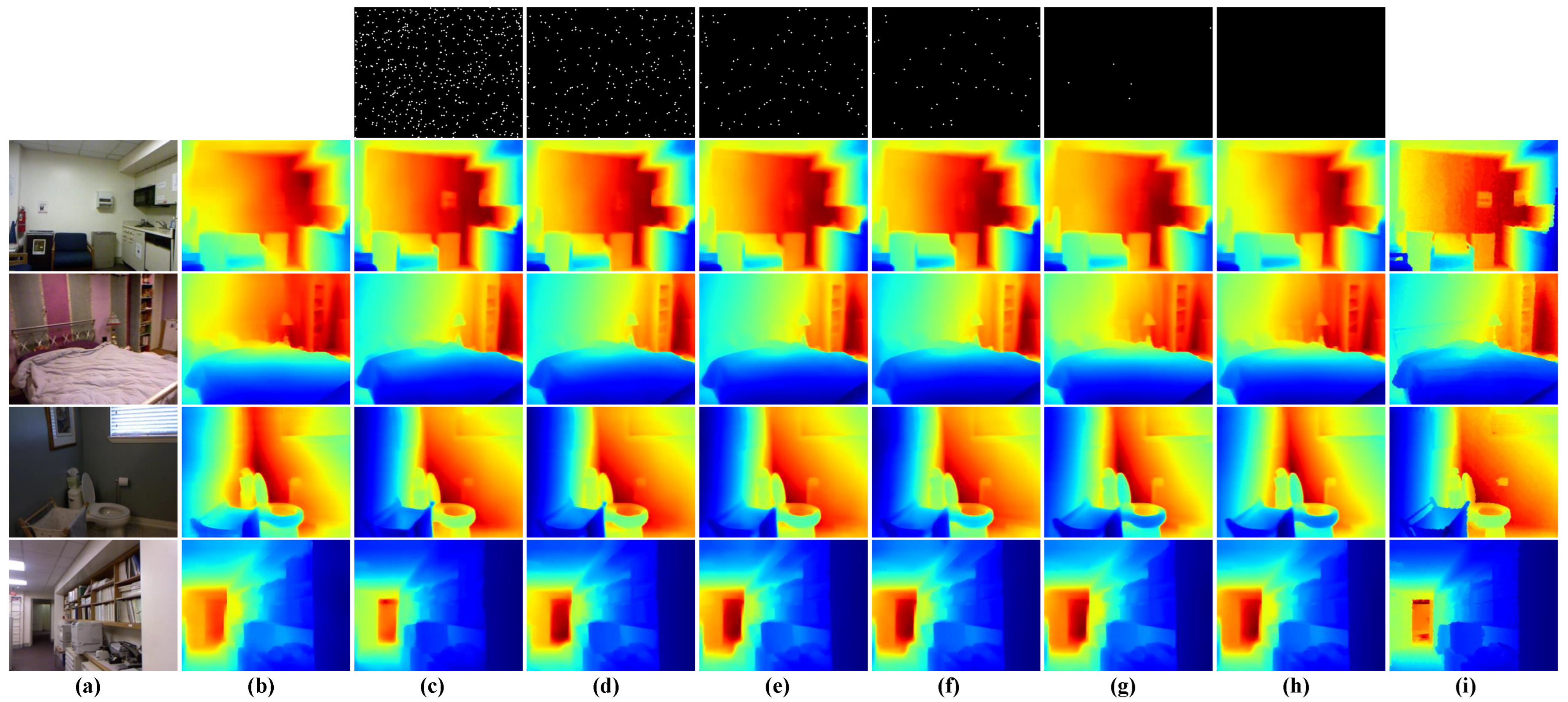
5.2. Visualization Results of the Model

To validate the generalization ability of our model to different levels of depth sparsity, we evaluated our full model’s performance across different input depth point counts: 500, 200, 100, 50, 5, and 0, and we visualized the resulting depth maps. As shown in Figure 5, the depth map output from the depth prediction branch in (b) already effectively reconstructs the depth structure of the entire scene. Across results (c) to (h), we observe that even with as few as 5 or 0 valid depth points in the sparse depth map, we still obtain meaningful depth map outputs. However, as the number of valid depth values decreases, the accuracy of absolute depth values decreases. For instance, in the first scenario, the protruding white object on the wall exhibits more significant depth accuracy in the 500-point depth map result compared to other sparsity levels. Observing the color contrast in the visualization results on the toilet in the third scenario, we notice a higher consistency between the depth results from 500 valid sparse points and the ground truth depth map values.

5.3. Ablation Studies

We conducted a series of ablation experiments to validate the effectiveness of the dual-branch architecture consisting of prediction and completion branches as well as the multi-scale local plane guidance module and loss functions. Additionally, for better visualization, we also show the line chart in Figure 6 to display the data from the corresponding ablation experiments in

Table 1. The performance obtained by different architectures (RMSE).

Models	500	200	100	50	5	0
DP branch	-	-	-	-	-	0.465
DC branch	0.125	0.160	0.199	0.245	0.416	0.516
Two branches	0.122	0.162	0.197	0.239	0.393	0.470

The optimal numerical results corresponding to sparse points are highlighted in bold.

,

Table 2. The performance obtained by the models with/without MLPGM (RMSE).

MLPGMDP	MLPGMDC	500	200	100	50	5	0
		0.123	0.164	0.203	0.251	0.411	0.488
✓		0.125	0.164	0.202	0.245	0.396	0.473
✓	✓	0.122	0.162	0.197	0.239	0.393	0.470

The optimal numerical results corresponding to sparse points are highlighted in bold.

and

Table 3. The performance obtained with different losses (RMSE).

Training Loss	500	200	100	50	5	0
$L_{SIL}+L_{MNL}$	0.125	0.167	0.208	0.260	0.401	0.464
$L_{SIL}+L_{GL}$	0.133	0.178	0.222	0.274	0.437	0.516
$L_{SIL}+L_{MNL}+L_{GL}$	0.122	0.162	0.197	0.239	0.393	0.470

The optimal numerical results corresponding to sparse points are highlighted in bold.

.

5.3.1. Effectiveness of the Dual-Branch Architecture

We first validated the effectiveness of the dual-branch architecture. We compared our full model with two variants of single branch models, and the experiment results are presented in Table 1. Here, “DP branch” (depth prediction branch) and “DC branch” (depth completion branch) represent the results obtained using only the depth prediction branch and only the depth completion branch, respectively. It is worth noting that to ensure fair comparison with the final model, the “DC branch” variant includes the encoder from the “DP branch” to utilize color image information for guidance during the processing. As shown in Table 1 and Figure 6a, firstly, when trained and tested using only the depth prediction model, it achieved the best numerical results as it focuses solely on the monocular depth estimation task. Secondly, compared to the single-branch depth completion model, the dual-branch network exhibited a significant improvement with 500 sparse points. Furthermore, the superiority of the dual-branch model became more pronounced as the number of valid depth points decreased to 50, 5, or even 0. Specifically, in scenarios where sparse depth points were absent, its performance could rival that of models dedicated solely to the depth prediction branch.

5.3.2. Effectiveness of the MLPGM

We then investigate the effectiveness of the multi-scale local plane guidance module. To this end, we compare the full model that integrates MLPGM in both decoders with two model variants: one that only integrates MLPGM in the depth prediction branch, and another that does not integrate MLPGM at all. Table 2 and Figure 6b present the results, indicating that the integration of MLPGM in both branches consistently outperforms other models across different input points.

5.3.3. Effectiveness of the Training Loss

We also examine the performance of our model trained with different losses. As we aim for our model to achieve good performance even when no depth is input, the inclusion of the $L_{SIL}$ loss is necessary. Therefore, we compare different loss variants, integrating either $L_{MNL}$ or $L_{GL}$ or both. The comparative results are presented in Table 3 and Figure 6c, showing that the model utilizing all three losses achieves the best performance in most cases.

5.4. Comparison to State of the Art

Finally, we compare our full model with five representative completion methods, namely pNCNN [80], CSPN [68], NLSPN [6], NConv-CNN [22], G2-MonoDepth [73] and SpAgNet [38], where NConv-CNN [22], G2-MonoDepth [73] and SpAgNet [38] are sparse invariant.

Table 4. Comparison with state-of-the-art methods (RMSE).

Methods	500	200	100	50	5	0
pNCNN  [80]	0.170	0.237	0.338	0.568	2.412	-
CSPN  [68]	0118	0.177	0.338	0.884	2.063	-
NLSPN  [6]	0.101	0.142	0.246	0.423	1.033	-
NConv-CNN  [22]	0.129	0.173	-	-	-	-
G2-MonoDepth  [73]	0.118	-	-	0.248	1.321	-
SpAgNet  [38]	0.114	0.155	0.209	0.272	0.469	-
Ours	0.122	0.162	0.197	0.239	0.393	0.470

The optimal numerical results correspond to sparse points, highlighted in bold; the next best are indicated with underlines; the third best are shown in italics.

demonstrates that our method outperforms all other methods when there are 100 input depth points or fewer.

5.5. Experimental Results in Real-World Application

In this section, we evaluate the model’s adaptability to depth maps with varying sparse distributions in real-world scenarios. To accomplish this, we utilized OPPO’s self-developed prototype equipped with Spot-iToF316 to capture both color images and sparse depth maps across various scenarios for testing purposes.

5.5.1. Testset

Speckle-type sparse ToF depth sensors can reduce the power consumption of the entire module by reducing the number of speckles, making them widely used in lightweight terminals such as smartphones. Speckle-type ToF cameras encounter common issues inherent in ToF cameras, including relatively low depth map resolution, black holes in the depth map due to objects beyond the hardware measurement range, occlusion and noise around object boundaries, as well as susceptibility to external environmental interference. Additionally, they possess unique characteristics: the depth maps obtained by speckle-type ToF cameras usually exhibit extremely high sparsity (typically less than 2% effective depth values). In this experiment, we used the OPPO Spot-iToF316 as the hardware device for acquiring sparse depth maps. We captured 180 sets of color images and corresponding sparse depth maps in different indoor scenes to create the test dataset. The resolution of both the color images and sparse depth maps in the test dataset is $256\times 192$.

5.5.2. Construction of Trainset

As obtaining corresponding ground-truth depth maps of Spot-iTOF for training is infeasible, we turn to virtual datasets. Among them, we specifically chose the Hypersim dataset, which contains scenes most similar to real-world scenarios and color images closest to actual images. The Hypersim dataset [81] is a large-scale synthetic dataset for computer vision and machine learning research, providing highly realistic indoor scenes. This dataset encompasses a variety of residential, commercial, and office environments, comprising 77,400 datasets across 461 indoor scenes, and it provides comprehensive scene information, including geometry, materials, depth, lighting, and semantic segmentation.

In this experimental section, we employed the Hypersim dataset for training and tested the model on the dataset acquired from OPPO’s Spot-iToF316 prototype. To achieve this, we preprocessed the Hypersim data as follows. Firstly, from the 77,400 datasets in Hypersim, we selected 38,542 sets of indoor scene data as the training set. Then, for the generation of color images, we utilized the lighting information in Hypersim and simulated different exposure settings to generate color images. The depth information provided by Hypersim represents the distance of object surfaces from the optical center; therefore, for the generation of dense depth maps, we utilized the camera intrinsic parameters to convert it into depth maps in terms of distances from objects to the image plane. Finally, to match the resolution of the test set, we downsampled both the color images and depth maps, adjusting them to the same resolution as OPPO’s, i.e., $256\times 192$. Bilinear downsampling was applied to the color images, while nearest-neighbor downsampling was applied to the depth maps to preserve depth values rather than generating pseudo-depth values.

Following the preliminary processing of the Hypersim dataset, we acquired a dataset comprising color images and corresponding ground-truth dense depth maps. To generate the sparse depth maps needed for training, we aimed to derive them from the ground-truth dense depth maps while ensuring that the resulting sparse depth maps closely resemble those obtained from iTOF depth sensors in real-world scenarios. Based on our observations of the basic characteristics of the depth value distribution of iTOF cameras in real-world scenes, we followed these steps to generate sparse depth maps.

• Step 1: The sparse depth map obtained from the iTOF sensor exhibits distinct distribution characteristics in rows and columns; thus, we first obtain a basic binary mask based on the fundamental row–column positions to represent the positions of valid depth points.
• Step 2: Considering that the sparse depth map generated by the iTOF sensor may not strictly adhere to the regular pattern of row–column positions due to inherent errors, we introduce random offsets to the positions in the basic binary mask to obtain a preliminary sparse mask.
• Step 3: We use the preliminary sparse mask to sample the dense depth map truth values, resulting in a preliminary sparse depth map.
• Step 4: Given that the sparse depth map obtained from the iTOF sensor may contain regions with missing depth values due to environmental factors, we generate random polygons in the sparse depth map to simulate these “black holes”.
• Step 5: Considering the randomness in the hardware measurement distance range, we randomly set the maximum value in the sparse depth map and filter out pixels exceeding this depth value.
• Step 6: Taking into account hardware noise and external interference, there may be deviations between the sparse depth map obtained from the iTOF sensor and the ground truth. We randomly add depth value offsets to the sparse depth points to simulate this noise.
• Step 7: Finally, considering the alignment issue between the color image and the sparse depth points, as well as potential noise near object edges, we randomly offset the positions of sparse depth points to simulate this scenario.

We illustrated the results of each step involved in obtaining the sparse depth map in Figure 7. Comparing (c) to (b), there is a slight shift in the positions of each mask point. From (d) to (e), noticeable “black hole” regions appear. Observing the discrepancy between (h) and (g), it can be seen that some valid points on the chair back in the foreground have shifted into the background. These results also confirm the accuracy of each step in our process.

5.5.3. Visualization Results of the OPPO Prototype Equipped with Spot-iToF316

Since the test set lacks ground-truth depth values, we only present the visualization results on the test set in Figure 8. From the visualization results, it can be observed that the model can effectively recover the scene structure and object edges. By observing the characteristics of sparse depth maps obtained from iTOF cameras and simulating these distribution characteristics when sampling from dense depth maps in Hypersim, the model performs well in dealing with different sparse distributions in the test set and achieves satisfactory results.

6. Conclusions

In conclusion, we have presented a depth completion model with high generalization capability, aimed at handling sparse depth maps with different sparse levels and irregular distributions, or even in cases where depth is extremely sparse or completely absent. Recognizing that as the number of valid depth points decreases, the depth completion task becomes a monocular depth estimation task, we combined the strengths of mainstream methods in both tasks and designed a dual-branch network structure consisting of the prediction branch and the completion branch, and we combined this with the commonly used 3D plane-related designs from the monocular depth estimation task, the multi-scale local plane guidance module and the mean normal loss function. These designs significantly improved the model’s performance in handling sparse depth inputs with different distributions. Finally, we conducted experiments on the benchmark NYU Depth V2 and the OPPO prototype dataset equipped with the Spot-iToF316 sensor in real-world applications. Our experiment demonstrates the effectiveness of our model, particularly in cases with limited, irregularly distributed or absent depth information.

References

1. Yan, Z.; Wang, K.; Li, X.; Zhang, Z.; Li, J.; Yang, J. RigNet: Repetitive image guided network for depth completion. In Proceedings of the European Conference on Computer Vision, Tel Aviv, Israel, 23–27 October 2022; Springer: Berlin/Heidelberg, Germany, 2022; pp. 214–230. [Google Scholar]
2. Ma, F.; Karaman, S. Sparse-to-dense: Depth prediction from sparse depth samples and a single image. In Proceedings of the 2018 IEEE International Conference on Robotics and Automation (ICRA), Brisbane, Australia, 21–25 May 2018; pp. 4796–4803. [Google Scholar]
3. Imran, S.; Liu, X.; Morris, D. Depth completion with twin surface extrapolation at occlusion boundaries. In Proceedings of the IEEE/CVF Conference on Computer Vision and Pattern Recognition, Nashville, TN, USA, 20–25 June 2021; IEEE: Piscataway, NJ, USA, 2021; pp. 2583–2592. [Google Scholar]
4. Qiu, J.; Cui, Z.; Zhang, Y.; Zhang, X.; Liu, S.; Zeng, B.; Pollefeys, M. Deeplidar: Deep surface normal guided depth prediction for outdoor scene from sparse lidar data and single color image. In Proceedings of the IEEE/CVF Conference on Computer Vision and Pattern Recognition, Long Beach, CA, USA, 15–20 June 2019; IEEE: Piscataway, NJ, USA, 2019; pp. 3313–3322. [Google Scholar]
5. Cheng, X.; Wang, P.; Guan, C.; Yang, R. Cspn++: Learning context and resource aware convolutional spatial propagation networks for depth completion. In Proceedings of the AAAI Conference on Artificial Intelligence, New York, NY, USA, 7–12 February 2020; Volume 34, pp. 10615–10622. [Google Scholar]
6. Park, J.; Joo, K.; Hu, Z.; Liu, C.K.; So Kweon, I. Non-local spatial propagation network for depth completion. In Proceedings of the European Conference on Computer Vision, Glasgow, UK, 23–28 August 2020; Springer: Berlin/Heidelberg, Germany, 2020; pp. 120–136. [Google Scholar]
7. Xu, Z.; Yin, H.; Yao, J. Deformable spatial propagation networks for depth completion. In Proceedings of the 2020 IEEE International Conference on Image Processing (ICIP), Virtual, 25–28 October 2020; IEEE: Piscataway, NJ, USA, 2020; pp. 913–917. [Google Scholar]
8. Lin, Y.; Cheng, T.; Zhong, Q.; Zhou, W.; Yang, H. Dynamic spatial propagation network for depth completion. In Proceedings of the AAAI, Virtual, 21–23 March 2022; pp. 1638–1646. [Google Scholar]
9. Liu, X.; Shao, X.; Wang, B.; Li, Y.; Wang, S. Graphcspn: Geometry-aware depth completion via dynamic gcns. In Proceedings of the European Conference on Computer Vision, Tel Aviv, Israel, 23–27 October 2022; Springer: Berlin/Heidelberg, Germany, 2022; pp. 90–107. [Google Scholar]
10. Tang, J.; Tian, F.P.; An, B.; Li, J.; Tan, P. Bilateral Propagation Network for Depth Completion. In Proceedings of the IEEE/CVF Conference on Computer Vision and Pattern Recognition, Seattle, WA, USA, 17–21 June 2024; pp. 9763–9772. [Google Scholar]
11. Chen, Y.; Yang, B.; Liang, M.; Urtasun, R. Learning joint 2d-3d representations for depth completion. In Proceedings of the IEEE/CVF International Conference on Computer Vision, Seoul, Republic of Korea, 27 October–2 November 2019; IEEE: Piscataway, NJ, USA, 2019; pp. 10023–10032. [Google Scholar]
12. Du, W.; Chen, H.; Yang, H.; Zhang, Y. Depth completion using geometry-aware embedding. In Proceedings of the 2022 International Conference on Robotics and Automation (ICRA), Philadelphia, PA, USA, 23–27 May 2022; pp. 8680–8686. [Google Scholar]
13. Wang, Y.; Sun, Y.; Liu, Z.; Sarma, S.E.; Bronstein, M.M.; Solomon, J.M. Dynamic graph cnn for learning on point clouds. Acm Trans. Graph. 2019, 38, 1–12. [Google Scholar] [CrossRef]
14. Su, H.; Jampani, V.; Sun, D.; Maji, S.; Kalogerakis, E.; Yang, M.H.; Kautz, J. Splatnet: Sparse lattice networks for point cloud processing. In Proceedings of the IEEE Conference on Computer Vision and Pattern Recognition, Salt Lake City, UT, USA, 18–23 June 2018; IEEE: Piscataway, NJ, USA, 2018; pp. 2530–2539. [Google Scholar]
15. Zhang, Y.; Guo, X.; Poggi, M.; Zhu, Z.; Huang, G.; Mattoccia, S. Completionformer: Depth completion with convolutions and vision transformers. In Proceedings of the IEEE/CVF Conference on Computer Vision and Pattern Recognition, Vancouver, BC, Canada, 17–24 June 2023; IEEE: Piscataway, NJ, USA, 2023; pp. 18527–18536. [Google Scholar]
16. Rho, K.; Ha, J.; Kim, Y. Guideformer: Transformers for image guided depth completion. In Proceedings of the IEEE/CVF Conference on Computer Vision and Pattern Recognition, New Orleans, LA, USA, 18–24 June 2022; IEEE: Piscataway, NJ, USA, 2022; pp. 6250–6259. [Google Scholar]
17. Wang, Y.; Li, B.; Zhang, G.; Liu, Q.; Gao, T.; Dai, Y. LRRU: Long-short Range Recurrent Updating Networks for Depth Completion. In Proceedings of the IEEE/CVF Conference on Computer Vision and Pattern Recognition, Vancouver, BC, Canada, 17–24 June 2023; IEEE: Piscataway, NJ, USA, 2023; pp. 9422–9432. [Google Scholar]
18. Uhrig, J.; Schneider, N.; Schneider, L.; Franke, U.; Brox, T.; Geiger, A. Sparsity invariant cnns. In Proceedings of the 2017 International Conference on 3D Vision (3DV), Qingdao, China, 10–12 October 2017; pp. 11–20. [Google Scholar]
19. Yin, W.; Zhang, J.; Wang, O.; Niklaus, S.; Chen, S.; Shen, C. Towards Domain-agnostic Depth Completion. arXiv 2022, arXiv:2207.14466. [Google Scholar]
20. Ryu, K.; Lee, K.i.; Cho, J.; Yoon, K.J. Scanline resolution-invariant depth completion using a single image and sparse LiDAR point cloud. IEEE Robot. Autom. Lett. 2021, 6, 6961–6968. [Google Scholar] [CrossRef]
21. Hua, J.; Gong, X. A normalized convolutional neural network for guided sparse depth upsampling. In Proceedings of the IJCAI, Stockholm, Sweden, 9–19 July 2018; pp. 2283–2290. [Google Scholar]
22. Eldesokey, A.; Felsberg, M.; Khan, F.S. Confidence propagation through cnns for guided sparse depth regression. IEEE Trans. Pattern Anal. Mach. Intell. 2019, 42, 2423–2436. [Google Scholar] [CrossRef] [PubMed]
23. Wang, T.H.; Wang, F.E.; Lin, J.T.; Tsai, Y.H.; Chiu, W.C.; Sun, M. Plug-and-play: Improve depth prediction via sparse data propagation. In Proceedings of the 2019 International Conference on Robotics and Automation (ICRA), Montreal, QC, Canada, 20–24 May 2019; pp. 5880–5886. [Google Scholar]
24. Long, Y.; Yu, H.; Liu, B. Depth completion towards different sensor configurations via relative depth map estimation and scale recovery. J. Vis. Commun. Image Represent. 2021, 80, 103272. [Google Scholar] [CrossRef]
25. Qi, X.; Liao, R.; Liu, Z.; Urtasun, R.; Jia, J. Geonet: Geometric neural network for joint depth and surface normal estimation. In Proceedings of the IEEE Conference on Computer Vision and Pattern Recognition, Salt Lake City, UT, USA, 18–23 June 2018; IEEE: Piscataway, NJ, USA, 2018; pp. 283–291. [Google Scholar]
26. Qi, X.; Liu, Z.; Liao, R.; Torr, P.H.; Urtasun, R.; Jia, J. Geonet++: Iterative geometric neural network with edge-aware refinement for joint depth and surface normal estimation. IEEE Trans. Pattern Anal. Mach. Intell. 2020, 44, 969–984. [Google Scholar] [CrossRef]
27. Yang, F.; Zhou, Z. Recovering 3d planes from a single image via convolutional neural networks. In Proceedings of the European Conference on Computer Vision (ECCV), Munich, Germany, 8–14 September 2018; pp. 85–100. [Google Scholar]
28. Li, B.; Huang, Y.; Liu, Z.; Zou, D.; Yu, W. StructDepth: Leveraging the structural regularities for self-supervised indoor depth estimation. In Proceedings of the IEEE/CVF International Conference on Computer Vision, Montreal, BC, Canada, 11–17 October 2021; pp. 12663–12673. [Google Scholar]
29. Long, X.; Lin, C.; Liu, L.; Li, W.; Theobalt, C.; Yang, R.; Wang, W. Adaptive surface normal constraint for depth estimation. In Proceedings of the IEEE/CVF International Conference on Computer Vision, Montreal, BC, Canada, 11–17 October 2021; pp. 12849–12858. [Google Scholar]
30. Lee, J.H.; Han, M.K.; Ko, D.W.; Suh, I.H. From big to small: Multi-scale local planar guidance for monocular depth estimation. arXiv 2019, arXiv:1907.10326. [Google Scholar]
31. Yin, W.; Liu, Y.; Shen, C.; Yan, Y. Enforcing geometric constraints of virtual normal for depth prediction. In Proceedings of the IEEE/CVF International Conference on Computer Vision, Seoul, Republic of Korea, 27 October–2 November 2019; IEEE: Piscataway, NJ, USA, 2019; pp. 5684–5693. [Google Scholar]
32. Yin, W.; Liu, Y.; Shen, C. Virtual normal: Enforcing geometric constraints for accurate and robust depth prediction. IEEE Trans. Pattern Anal. Mach. Intell. 2021, 44, 7282–7295. [Google Scholar] [CrossRef]
33. Yang, X.; Ma, Z.; Ji, Z.; Ren, Z. Gedepth: Ground embedding for monocular depth estimation. In Proceedings of the IEEE/CVF International Conference on Computer Vision, Paris, France, 2–3 October 2023; pp. 12719–12727. [Google Scholar]
34. Patil, V.; Sakaridis, C.; Liniger, A.; Van Gool, L. P3Depth: Monocular Depth Estimation with a Piecewise Planarity Prior. In Proceedings of the IEEE/CVF Conference on Computer Vision and Pattern Recognition, New Orleans, LA, USA, 18–24 June 2022; IEEE: Piscataway, NJ, USA, 2022; pp. 1610–1621. [Google Scholar]
35. Hu, M.; Wang, S.; Li, B.; Ning, S.; Fan, L.; Gong, X. Penet: Towards precise and efficient image guided depth completion. In Proceedings of the 2021 IEEE International Conference on Robotics and Automation (ICRA), Xi’an, China, 30 May–5 June 2021; pp. 13656–13662. [Google Scholar]
36. Van Gansbeke, W.; Neven, D.; De Brabandere, B.; Van Gool, L. Sparse and noisy lidar completion with rgb guidance and uncertainty. In Proceedings of the 2019 16th International Conference on Machine Vision Applications (MVA), Tokyo, Japan, 27–31 May 2019; pp. 1–6. [Google Scholar]
37. Silberman, N.; Hoiem, D.; Kohli, P.; Fergus, R. Indoor segmentation and support inference from rgbd images. ECCV (5) 2012, 7576, 746–760. [Google Scholar]
38. Conti, A.; Poggi, M.; Mattoccia, S. Sparsity Agnostic Depth Completion. In Proceedings of the IEEE/CVF Winter Conference on Applications of Computer Vision, Waikoloa, HI, USA, 2–7 January 2023; pp. 5871–5880. [Google Scholar]
39. Lee, J.H.; Kim, C.S. Multi-loss rebalancing algorithm for monocular depth estimation. In Proceedings of the European Conference on Computer Vision, Glasgow, UK, 23–28 August 2020; Springer: Berlin/Heidelberg, Germany, 2020; pp. 785–801. [Google Scholar]
40. Eigen, D.; Puhrsch, C.; Fergus, R. Depth map prediction from a single image using a multi-scale deep network. Adv. Neural Inf. Process. Syst. 2014, 27, 1–9. [Google Scholar]
41. Fu, H.; Gong, M.; Wang, C.; Batmanghelich, K.; Tao, D. Deep ordinal regression network for monocular depth estimation. In Proceedings of the IEEE Conference on Computer Vision and Pattern Recognition, Salt Lake City, UT, USA, 18–23 June 2018; IEEE: Piscataway, NJ, USA, 2018; pp. 2002–2011. [Google Scholar]
42. Bhat, S.F.; Alhashim, I.; Wonka, P. Adabins: Depth estimation using adaptive bins. In Proceedings of the IEEE/CVF Conference on Computer Vision and Pattern Recognition, Nashville, TN, USA, 20–25 June 2021; IEEE: Piscataway, NJ, USA, 2021; pp. 4009–4018. [Google Scholar]
43. Agarwal, A.; Arora, C. Attention attention everywhere: Monocular depth prediction with skip attention. In Proceedings of the IEEE/CVF Winter Conference on Applications of Computer Vision, Waikoloa, HI, USA, 2–7 January 2023; pp. 5861–5870. [Google Scholar]
44. Qu, C.; Nguyen, T.; Taylor, C. Depth completion via deep basis fitting. In Proceedings of the IEEE/CVF Winter Conference on Applications of Computer Vision, Snowmass Village, CO, USA, 1–5 March 2020; pp. 71–80. [Google Scholar]
45. Senushkin, D.; Romanov, M.; Belikov, I.; Patakin, N.; Konushin, A. Decoder modulation for indoor depth completion. In Proceedings of the 2021 IEEE/RSJ International Conference on Intelligent Robots and Systems (IROS), Prague, Czech Republic, 27 September–1 October 2021; IEEE: Piscataway, NJ, USA, 2021; pp. 2181–2188. [Google Scholar]
46. Imran, S.; Long, Y.; Liu, X.; Morris, D. Depth coefficients for depth completion. In Proceedings of the 2019 IEEE/CVF Conference on Computer Vision and Pattern Recognition (CVPR), Long Beach, CA, USA, 15–20 June 2019; IEEE: Piscataway, NJ, USA, 2019; pp. 12438–12447. [Google Scholar]
47. Ma, F.; Cavalheiro, G.V.; Karaman, S. Self-supervised sparse-to-dense: Self-supervised depth completion from lidar and monocular camera. In Proceedings of the 2019 International Conference on Robotics and Automation (ICRA), Montreal, QC, Canada, 20–24 May 2019; pp. 3288–3295. [Google Scholar]
48. Zhang, Y.; Nguyen, T.; Miller, I.D.; Shivakumar, S.S.; Chen, S.; Taylor, C.J.; Kumar, V. Dfinenet: Ego-motion estimation and depth refinement from sparse, noisy depth input with rgb guidance. arXiv 2019, arXiv:1903.06397. [Google Scholar]
49. Jaritz, M.; De Charette, R.; Wirbel, E.; Perrotton, X.; Nashashibi, F. Sparse and dense data with cnns: Depth completion and semantic segmentation. In Proceedings of the 2018 International Conference on 3D Vision (3DV), Verona, Italy, 5–8 September 2018; pp. 52–60. [Google Scholar]
50. Shivakumar, S.S.; Nguyen, T.; Miller, I.D.; Chen, S.W.; Kumar, V.; Taylor, C.J. Dfusenet: Deep fusion of rgb and sparse depth information for image guided dense depth completion. In Proceedings of the 2019 IEEE Intelligent Transportation Systems Conference (ITSC), Auckland, New Zealand, 27–30 October 2019; IEEE: Piscataway, NJ, USA, 2019; pp. 13–20. [Google Scholar]
51. Fu, C.; Dong, C.; Mertz, C.; Dolan, J.M. Depth completion via inductive fusion of planar lidar and monocular camera. In Proceedings of the 2020 IEEE/RSJ International Conference on Intelligent Robots and Systems (IROS), Las Vegas, NV, USA, 25–29 October 2020; IEEE: Piscataway, NJ, USA, 2020; pp. 10843–10848. [Google Scholar]
52. Zhong, Y.; Wu, C.Y.; You, S.; Neumann, U. Deep rgb-d canonical correlation analysis for sparse depth completion. Adv. Neural Inf. Process. Syst. 2019, 32, 1–11. [Google Scholar]
53. Yang, X.; Liu, W.; Tao, D.; Cheng, J. Canonical correlation analysis networks for two-view image recognition. Inf. Sci. 2017, 385, 338–352. [Google Scholar] [CrossRef]
54. Mao, X.; Shen, C.; Yang, Y.B. Image restoration using very deep convolutional encoder-decoder networks with symmetric skip connections. Adv. Neural Inf. Process. Syst. 2016, 29, 1–9. [Google Scholar]
55. Zhou, Z.; Siddiquee, M.M.R.; Tajbakhsh, N.; Liang, J. Unet++: Redesigning skip connections to exploit multiscale features in image segmentation. IEEE Trans. Med. Imaging 2019, 39, 1856–1867. [Google Scholar] [CrossRef] [PubMed]
56. Zhang, Y.; Wei, P.; Li, H.; Zheng, N. Multiscale adaptation fusion networks for depth completion. In Proceedings of the 2020 International Joint Conference on Neural Networks (IJCNN), Glasgow, UK, 19–24 July 2020; IEEE: Piscataway, NJ, USA, 2020; pp. 1–7. [Google Scholar]
57. Li, A.; Yuan, Z.; Ling, Y.; Chi, W.; Zhang, S.; Zhang, C. A multi-scale guided cascade hourglass network for depth completion. In Proceedings of the IEEE/CVF Winter Conference on Applications of Computer Vision, Snowmass Village, CO, USA, 1–5 March 2020; pp. 32–40. [Google Scholar]
58. Tang, J.; Tian, F.P.; Feng, W.; Li, J.; Tan, P. Learning guided convolutional network for depth completion. IEEE Trans. Image Process. 2020, 30, 1116–1129. [Google Scholar] [CrossRef] [PubMed]
59. Schuster, R.; Wasenmuller, O.; Unger, C.; Stricker, D. Ssgp: Sparse spatial guided propagation for robust and generic interpolation. In Proceedings of the IEEE/CVF Winter Conference on Applications of Computer Vision, Waikoloa, HI, USA, 3–8 January 2021; pp. 197–206. [Google Scholar]
60. Dimitrievski, M.; Veelaert, P.; Philips, W. Learning morphological operators for depth completion. In Advanced Concepts for Intelligent Vision Systems: Proceedings of the 19th International Conference, ACIVS 2018, Poitiers, France, 24–27 September 2018; Proceedings 19; Springer: Berlin/Heidelberg, Germany, 2018; pp. 450–461. [Google Scholar]
61. Hambarde, P.; Murala, S. S2DNet: Depth estimation from single image and sparse samples. IEEE Trans. Comput. Imaging 2020, 6, 806–817. [Google Scholar] [CrossRef]
62. Chen, Z.; Badrinarayanan, V.; Drozdov, G.; Rabinovich, A. Estimating depth from rgb and sparse sensing. In Proceedings of the European Conference on Computer Vision (ECCV), Munich, Germany, 8–14 September 2018; pp. 167–182. [Google Scholar]
63. Hegde, G.; Pharale, T.; Jahagirdar, S.; Nargund, V.; Tabib, R.A.; Mudenagudi, U.; Vandrotti, B.; Dhiman, A. Deepdnet: Deep dense network for depth completion task. In Proceedings of the IEEE/CVF Conference on Computer Vision and Pattern Recognition, Nashville, TN, USA, 20–25 June 2021; IEEE: Piscataway, NJ, USA, 2021; pp. 2190–2199. [Google Scholar]
64. Liao, Y.; Huang, L.; Wang, Y.; Kodagoda, S.; Yu, Y.; Liu, Y. Parse geometry from a line: Monocular depth estimation with partial laser observation. In Proceedings of the 2017 IEEE International Conference on Robotics and Automation (ICRA), Singapore, 29 May–3 June 2017; pp. 5059–5066. [Google Scholar]
65. Gu, J.; Xiang, Z.; Ye, Y.; Wang, L. Denselidar: A real-time pseudo dense depth guided depth completion network. IEEE Robot. Autom. Lett. 2021, 6, 1808–1815. [Google Scholar] [CrossRef]
66. Zhu, Y.; Dong, W.; Li, L.; Wu, J.; Li, X.; Shi, G. Robust depth completion with uncertainty-driven loss functions. In Proceedings of the AAAI Conference on Artificial Intelligence, Vancouver, BC, Canada, 20–27 February 2024; Volume 36, pp. 3626–3634. [Google Scholar]
67. Zhang, Y.; Wei, P.; Zheng, N. A multi-cue guidance network for depth completion. Neurocomputing 2021, 441, 291–299. [Google Scholar] [CrossRef]
68. Cheng, X.; Wang, P.; Yang, R. Depth estimation via affinity learned with convolutional spatial propagation network. In Proceedings of the European Conference on Computer Vision (ECCV), Munich, Germany, 8–14 September 2018; pp. 103–119. [Google Scholar]
69. Jeon, Y.; Kim, H.; Seo, S.W. ABCD: Attentive Bilateral Convolutional Network for Robust Depth Completion. IEEE Robot. Autom. Lett. 2021, 7, 81–87. [Google Scholar] [CrossRef]
70. Xiong, X.; Xiong, H.; Xian, K.; Zhao, C.; Cao, Z.; Li, X. Sparse-to-dense depth completion revisited: Sampling strategy and graph construction. In Proceedings of the European Conference on Computer Vision, Glasgow, UK, 23–28 August 2020; Springer: Berlin/Heidelberg, Germany, 2020; pp. 682–699. [Google Scholar]
71. Zhao, S.; Gong, M.; Fu, H.; Tao, D. Adaptive context-aware multi-modal network for depth completion. IEEE Trans. Image Process. 2021, 30, 5264–5276. [Google Scholar] [CrossRef] [PubMed]
72. Xu, Y.; Zhu, X.; Shi, J.; Zhang, G.; Bao, H.; Li, H. Depth completion from sparse lidar data with depth-normal constraints. In Proceedings of the IEEE/CVF International Conference on Computer Vision, Seoul, Republic of Korea, 27 October–2 November 2019; IEEE: Piscataway, NJ, USA, 2019; pp. 2811–2820. [Google Scholar]
73. Wang, H.; Yang, M.; Zheng, N. G2-MonoDepth: A General Framework of Generalized Depth Inference from Monocular RGB+ X Data. IEEE Trans. Pattern Anal. Mach. Intell. 2023, 46, 3753–3771. [Google Scholar] [CrossRef] [PubMed]
74. Hu, M. Towards precise and robust depth completion. Master’s Thesis, Zhejiang University, Hangzhou, China, 2021. [Google Scholar]
75. He, K.; Zhang, X.; Ren, S.; Sun, J. Deep residual learning for image recognition. In Proceedings of the IEEE Conference on Computer Vision and Pattern Recognition, Las Vegas, NV, USA, 26 June–1 July 2016; pp. 770–778. [Google Scholar]
76. Yang, M.; Yu, K.; Zhang, C.; Li, Z.; Yang, K. Denseaspp for semantic segmentation in street scenes. In Proceedings of the IEEE Conference on Computer Vision and Pattern Recognition, Salt Lake City, UT, USA, 18–23 June 2018; IEEE: Piscataway, NJ, USA, 2018; pp. 3684–3692. [Google Scholar]
77. Paszke, A.; Gross, S.; Massa, F.; Lerer, A.; Bradbury, J.; Chanan, G.; Killeen, T.; Lin, Z.; Gimelshein, N.; Antiga, L.; et al. PyTorch: An Imperative Style, High-Performance Deep Learning Library. In Proceedings of the NeuroIPS, Vancouver, BC, Canada, 8–14 December 2019. [Google Scholar]
78. Kingma, D.; Ba, J. Adam: A method for stochastic optimization. arXiv 2014, arXiv:1412.6980. [Google Scholar]
79. Ishii, Y.; Yamashita, T. Cutdepth: Edge-aware data augmentation in depth estimation. arXiv 2021, arXiv:2107.07684. [Google Scholar]
80. Eldesokey, A.; Felsberg, M.; Holmquist, K.; Persson, M. Uncertainty-aware cnns for depth completion: Uncertainty from beginning to end. In Proceedings of the IEEE/CVF Conference on Computer Vision and Pattern Recognition, Seattle, WA, USA, 13–19 June 2020; IEEE: Piscataway, NJ, USA, 2020; pp. 12014–12023. [Google Scholar]
81. Roberts, M.; Ramapuram, J.; Ranjan, A.; Kumar, A.; Bautista, M.A.; Paczan, N.; Webb, R.; Susskind, J.M. Hypersim: A photorealistic synthetic dataset for holistic indoor scene understanding. In Proceedings of the IEEE/CVF International Conference on Computer Vision, Montreal, BC, Canada, 11–17 October 2021; pp. 10912–10922. [Google Scholar]
Figure 1. Network architectures for guided depth completion.
Algorithms 17 00298 g001
Figure 2. An overview of our sparse-invariant model. It is a dual-branch encoder–decoder architecture with an integration of multi-scale local planar guidance modules in two decoders.
Algorithms 17 00298 g002
Figure 3. Diagram illustrating the upsampling of plane coefficients. Regions with the same color and numerical values represent the same plane coefficients, indicating that the upsampled results maintain consistency in plane coefficients within local regions.
Algorithms 17 00298 g003
Figure 4. Visualization of model training process.
Algorithms 17 00298 g004
Figure 5. The visualization results obtained by our full model when the input depth points vary from 500 to 200, 100, 50 and 0 (shown in (ch)). (a): color image, (b): the intermediate depth map obtained by the prediction branch, (i): the ground truth depth map. The depth map was visualized using the “jet” colormap.
Algorithms 17 00298 g005
Figure 6. The visualization of ablation studies results. (a) The performance of different architectures, (b) The performance of the models with/without MLPGM, (c) The performance of different losses.
Algorithms 17 00298 g006
Figure 7. Sparse depth map generation illustration: (a) color image, (bh) results of obtaining the sparse depth map at each step. (A dilation operation on the sparse depth map was performed for better visualization.)
Algorithms 17 00298 g007
Figure 8. Visualization results of the OPPO prototype equipped with Spot-iToF316. (a): Color image and corresponding sparse depth (a dilation operation on the sparse depth map was performed for better visualization). (b): Predicted depth map.
Algorithms 17 00298 g008