Abstract
Remaining useful life (RUL) prediction is widely applied in prognostic and health management (PHM) of turbofan engines. Although some of the existing deep learning-based models for RUL prediction of turbofan engines have achieved satisfactory results, there are still some challenges. For example, the spatial features and importance differences hidden in the raw monitoring data are not sufficiently addressed or highlighted. In this paper, a novel multi-head self-Attention fully convolutional network (MSA-FCN) is proposed for predicting the RUL of turbofan engines. MSA-FCN combines a fully convolutional network and multi-head structure, focusing on the degradation correlation among various components of the engine and extracting spatially characteristic degradation representations. Furthermore, by introducing dual multi-head self-attention modules, MSA-FCN can capture the differential contributions of sensor data and extracted degradation representations to RUL prediction, emphasizing key data and representations. The experimental results on the C-MAPSS dataset demonstrate that, under various operating conditions and failure modes, MSA-FCN can effectively predict the RUL of turbofan engines. Compared with 11 mainstream deep neural networks, MSA-FCN achieves competitive advantages in terms of both accuracy and timeliness for RUL prediction, delivering more accurate and reliable forecasts.
1. Introduction
Prognosis and health management (PHM) has become increasingly important for full and effective use of equipment (such as turbofan engines, high-speed Computerized Numerical Control (CNC) milling machines, high-intensity radiation field batteries, etc.) in modern manufacturing industries as the amount and complexity of industrial equipment increases, and it provides valuable references and recommendations for maintenance planning and improvement of equipment. Remaining useful life (RUL) prediction is the core and fundamental work in PHM. By accurately predicting the RUL of equipment, sudden or potential failures can be effectively avoided, thus optimizing maintenance strategies and reducing maintenance costs. As a result, research on accurate RUL prediction approaches has strongly attracted the attention of academia and industry. These approaches fall into two main categories, namely, model-based and data-driven approaches.
Through the experience of experts and prior knowledge of the equipment, model-based approaches create mathematical or physical models that incorporate degradation mechanisms and reflect degradation trends. Hu et al. [1] proposed an integrated method based on the Gauss–Hermite particle filter technique to predict the capacity and RUL of lithium-ion batteries. Qian et al. [2] proposed a multi-timescale modeling approach to predict the RUL of rolling bearings by integrating an enhanced phase space warping with a modified Paris crack growth model. Thelen et al. [3] proposed an enhanced empirical model-based prediction approach with probabilistic data-driven error correction for the RUL prediction of batteries. With the increasing complexity of equipment and systems in modern industries, it is becoming increasingly difficult and impractical to build these models that can precisely understand degradation trends and rules. In addition, since the equipment used in different application scenarios has unique degradation mechanisms, it is difficult to apply a model built for one case to the same equipment in other applications. Therefore, the disadvantage of the model-based method is that it is less practical and flexible.
With the rapid advancement in sensor technology and signal processes, data-driven methods have gradually become a research hotspot in the field of RUL prediction. Data-driven methods extract degradation features and information from the massive raw monitoring data gathered by diverse sensors installed on the equipment, aiming to establish the mappings between the monitoring data and corresponding RUL. Data-driven methods based on artificial intelligence have become increasingly popular, mainly including methods based on conventional machine learning (CML) and deep learning (DL).
CML-based approaches use shallow machine learning algorithms for feature learning and regression to obtain degradation information from monitoring data and create the corresponding mappings to achieve the goal of RUL prediction. Aye and Heyns [4] proposed an optimal Gaussian process regression approach to predict the RUL of slow speed bearings. Benkedjouh et al. [5] combined support vector regression with the ISOMAP feature reduction technique to predict the RUL of bearings. Wu et al. [6] utilized random a forest model for tool wear prediction. Javed et al. [7] proposed a prognostic model combining the summation wavelet-extreme learning machine and subtractive-maximum entropy fuzzy clustering to predict the RUL of turbofan engines. Yan et al. [8] proposed a hidden semi-Markov model-based approach for the RUL prediction of air-handling systems and their components. The performance of CML-based methods relies heavily on feature extraction and selection, which requires strong support from domain experts and expertise about the related equipment.
Deep learning-based RUL prediction methods [9,10,11,12,13,14,15,16,17,18,19] can automatically learn various features and deep-level representations from a large amount of raw data through deep neural networks, which effectively overcomes the shortcomings of CML-based approaches. In the field of RUL prediction for tools, Li et al. [20] proposed a dual-module methodology framework that integrates the following two core modules: detection and regression. The detection module relies on a lightweight convolutional neural network called WearNet, which exhibits excellent classification accuracy while maintaining a small model size and fast detection speed. To further enhance WearNet’s performance, the framework incorporates transfer learning techniques, utilizing its training on a new database to accelerate model convergence. Additionally, the regression module of the framework adopts a Bidirectional Long Short-Term Memory (BiLSTM) structure. This structure captures temporal relationships more comprehensively by processing sequence data in both directions, enabling precise RUL prediction tasks. It is worth mentioning that the regression module also offers the following two prediction modes: standard and hybrid. The latter integrates the wear detection results from WearNet, providing richer information input for prediction. In the domain of RUL prediction for turbofan engines, Kim et al. [21] presented a Transformer-based RUL prediction model. This model employs the encoder structure of Transformer [22] combined with a multi-head self-attention module and a feed-forward layer to effectively capture long-term dependencies in the data. To address data imbalance issues, the model specifically introduces an adaptive RUL reweighting strategy. This strategy dynamically adjusts the sample weights of different RUL categories based on errors during the training process, allowing the model to focus more on difficult-to-learn samples. Finally, the model adopts kernel smoothing techniques to ensure the continuity of the target RUL, further enhancing the accuracy and robustness of its RUL predictions. In the area of RUL prediction for bearings, Zhou and Tang [23] constructed a comprehensive bearing failure prediction framework. This framework integrates sequential time-domain signal preprocessing, feature extraction and a physically informed wavelet neural network. It forms new time series data through signal segmentation and statistical indicator calculation. Furthermore, it employs empirical mode decomposition to mine the critical features of bearing degradation deeply. Moreover, the framework introduces a wavelet neural network with a wavelet basis as the activation function. This network can more effectively process the features extracted by empirical mode decomposition, enabling more accurate RUL predictions.
Similarly, RUL prediction methods for turbofan engines based on deep learning has attracted much attention because of its excellent ability to process high-dimensional and nonlinear data. Some existing approaches mainly focus on extracting temporal features from raw monitoring data, and the extracted features essentially reflect the degradation trend in the turbofan engines. Song et al. [24] employed LSTM to form a bi-level framework to process time series characteristics. Xiao et al. [25] used LSTM to learn temporal features based on feature reconstruction, and the learned features were enhanced by noise injection. Li et al. [26] proposed a multi-scale Deep Convolutional Neural Network (DCNN) that can simultaneously extract temporal features at different scales from raw monitoring data. Chen et al. [27] utilized and modified LSTM to capture temporal features of multiple time steps from raw monitoring data. Meanwhile, in raw monitoring data, different sensor data and learned representations contain degradation information of varying importance, and they contribute unequally to the RUL prediction of turbofan engines. Therefore, some works have aimed to capture and strengthen these important data and representations. Liu et al. [28] proposed a single-feature attention mechanism that assigns greater weights to more important sensor data. Xiang et al. [29] utilized a single attention mechanism to enhance temporal features obtained by multiple multicellular LSTM units. Wang et al. [30] constructed a squeeze–excitation unit that can capture and augment informative feature mappings extracted by separable convolutional layers. Fan et al. [31] established a single-trend attention network that is able to characterize each sensor data point effectively.
The aforementioned deep learning-based prediction models for the RUL of turbofan engines have achieved certain results, but they have not paid attention to the following factors when extracting degradation representations under multiple operating conditions and failure modes:
- Spatial characteristics within multi-sensor data. The operation of a turbofan engine is a result of the collaborative work of its various components. The degradation of one component can lead to the degradation of related components, and the degradation of other components can exacerbate the degradation of that component. These degradation correlations among components are mapped as spatial characteristics within multi-sensor data. Ignoring the corresponding spatial characteristics under multiple operating conditions and failure modes can lead to an insufficient understanding of equipment degradation behavior by the prediction model, which may negatively impact the prediction accuracy of the model.
- Differences in importance among sensor data and representations. Each sensor point and each extracted representation contributes differently to RUL prediction. In other words, there are differences in their importance to prediction accuracy. Considering only the differences in importance within sensor data or representations under multiple operating conditions and failure modes can lead to the prediction model failing to enhance a portion of important data and representations, which may reduce the accuracy of the model’s RUL prediction.
Based on the consideration of the aforementioned factors, this paper proposes a multi-head self-attention-based fully convolutional network (MSA-FCN) for predicting the RUL of turbofan engines. Firstly, the multi-head fully convolutional neural network (MHFCN) is constructed in MSA-FCN. This module employs multiple fully convolutional networks to perform convolution operations on the input along the sensor and spatial dimensions, aiming to extract degradation representations with spatial characteristics. Meanwhile, MHFCN organizes these fully convolutional networks using the multi-head structure of Transformer, enabling the module to enhance the richness of its extracted representations from different aspects of data. Secondly, the dual multi-head self-attention module (DMSAM) is constructed in MSA-FCN. It performs multi-head self-attention weighting operations on the input along the sensor and spatial dimensions, respectively, aiming to enhance the parts that are valuable for RUL prediction in samples and representations. Specifically, the multi-head sensor data self-attention module within DMSAM assigns heavier weights to important sensor data through the self-attention mechanism along the sensor dimension and utilizes the multi-head structure to improve the richness of the weighted data. The multi-head spatial feature self-attention module within DMSAM assigns heavier weights to the important degradation representations with spatial characteristics through the self-attention mechanism along the spatial dimension and similarly uses the multi-head structure to enhance the richness of the weighted representations. Finally, a multilayer perceptron module within MSA-FCN integrates all the extracted degradation representations to output the predicted RUL value. This paper performs RUL prediction experiments using turbine engine datasets containing multiple operational conditions and fault modes to evaluate the performance of MSA-FCN. The major contributions of our paper are as follows:
(1) This paper proposes a multi-head self-attention-based fully convolutional network (MSA-FCN) for RUL prediction. On the one hand, its multi-head fully convolutional network (MHFCN) can sufficiently capture and learn degradation representations with spatial features. On the other hand, its dual multi-head self-attention modules (DMSAMs) can effectively learn and capture the importance differences present in the sensor data and the learned representations. Moreover, the multi-head structure of the proposed model is able to make the learned degradation information richer and more comprehensive.
(2) This paper verifies the effectiveness of the components and multi-head structure of MSA-FCN through a series of ablation experiments. The experimental results demonstrate that MHFCN, DMSAM, and the multi-head structure allow MSA-FCN to achieve accurate and stable RUL prediction results. Further, performance comparisons with other models are also conducted, and the results show that MSA-FCN has advantages over 11 existing deep neural networks for predicting RUL on the same datasets and has a better overall prediction performance than these models.
This paper is organized into the following sections. The related work is introduced in Section 2. Subsequently, MSA-FCN is interpreted in Section 3. Then, the RUL prediction experiments of MSA-FCN are reported in Section 4. The comparison and discussion of MSA-FCN are presented in Section 5. Finally, the conclusion is summarized in Section 6.
2. Related Work
Compared with the conventional attention mechanism, Transformer’s multi-head self-attention mechanism [22] has the advantage of being able to focus adequately on various aspects of the data and the internal correlations of the data. More importantly, the mechanism as a joint strategy allows the corresponding neural network to learn rich associations and information from different sub-representation spaces at different positions.
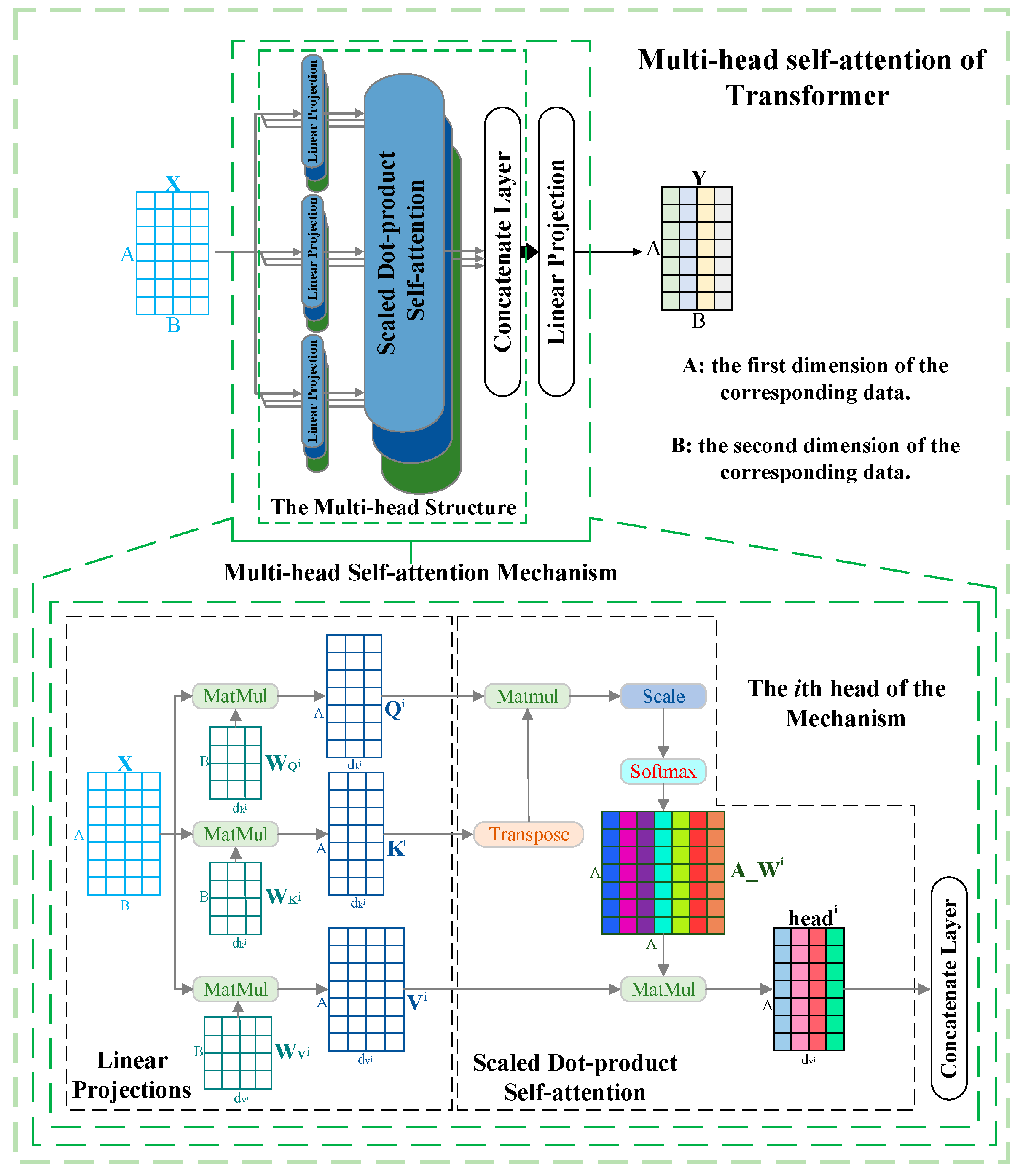
The forward propagation of the multi-head self-attention of Transformer is described as follows. First, in each head, input data are transformed by three linear projections and then fed into the scaled dot-product self-attention to obtain the attention weights assigned to the corresponding data. Then, a concatenate layer is utilized to fuse the weighted data of all the heads, which forms the multi-head structure. After that, a linear projection is adopted to change the fused output into the same shape as the input data . Subsequently, a residual connection [32] is applied to connect the reshaped output and the input data . Finally, layer normalization [33] is used to regulate the output of the residual connection operation to generate the final output . The above processes can be mathematically expressed as Equations (1)–(6).
where, in the th head, , , , , , , and represent the query matrix, key matrix, value matrix, transpose operation, scaling factor, attention weights, and corresponding weighted data, respectively. , , , and denote linear projections that are trainable parameters. The multi-head self-attention is shown in Figure 1.
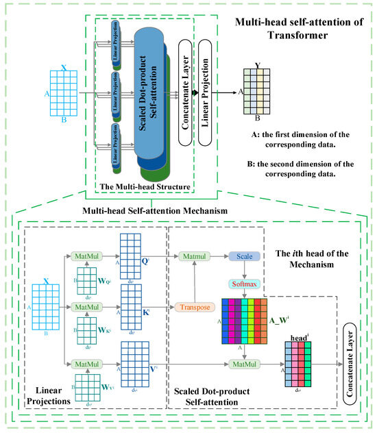
Figure 1.
Diagram of multi-head self-attention.
3. The Proposed Neural Network
This paper proposes a novel multi-head self-attention-based fully convolutional network (MSA-FCN) for the RUL prediction of turbofan engines. Firstly, this paper constructs the multi-head fully convolutional network (MHFCN), which performs convolutional operations along both the sensor dimension and spatial dimension to learn valuable and rich degradation representations with spatial characteristics. Secondly, this paper constructs the dual multi-head self-attention module (DMSAM) to capture the importance differences that exist in both the sensor data and extracted representations and to enhance the degradation information that can contribute significantly to RUL. Based on MHFCN and DMSAM, MSA-FCN can extract useful and comprehensive degradation representations from monitoring data containing multiple fault modes and operating conditions and use these representations to predict RUL results.
3.1. Task Statement
The RUL prediction of equipment is essentially a classical regression task based on a large amount of raw monitoring data containing both historical and real-time data. Therefore, the proposed neural network serves as a deep supervised learning-based regression approach to achieve RUL prediction.
Firstly, the raw monitoring data are transformed and divided to a training dataset and a testing dataset, as shown in Equations (7) and (8), where represents sequence length of the data.
where , , , , , and represent the th training sample, the th RUL training label, the th testing sample, the th RUL testing label, the number of training samples, and the number of testing samples, respectively. After that, a neural network is established and trained by continuously narrowing the gap between the label of training sample and the corresponding predicted RUL . Finally, the trained neural network predicts the RUL of testing sample , and the difference between the label and the predicted value is also calculated to evaluate the performance of the neural network.
3.2. Architecture of MSA-FCN
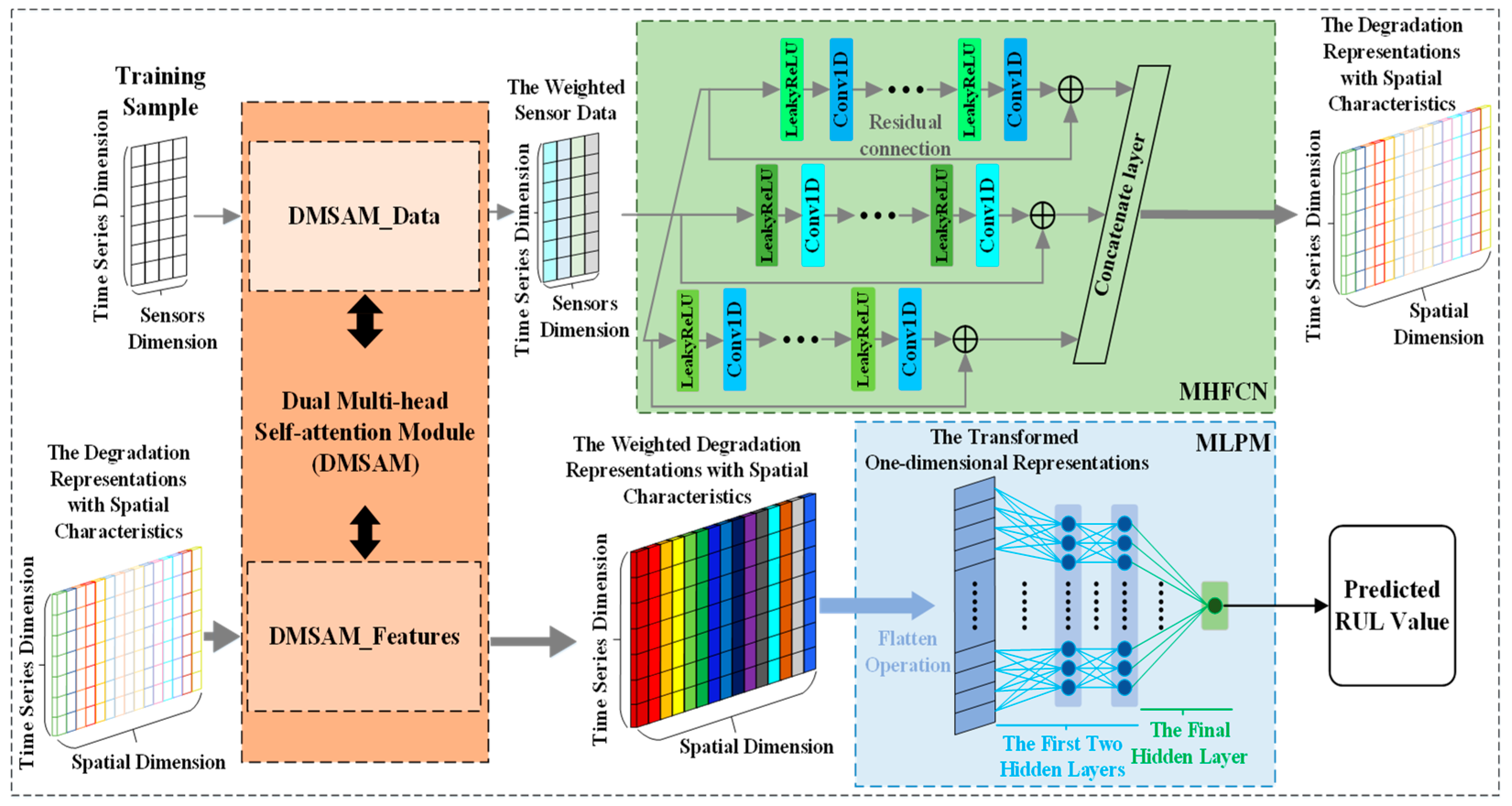
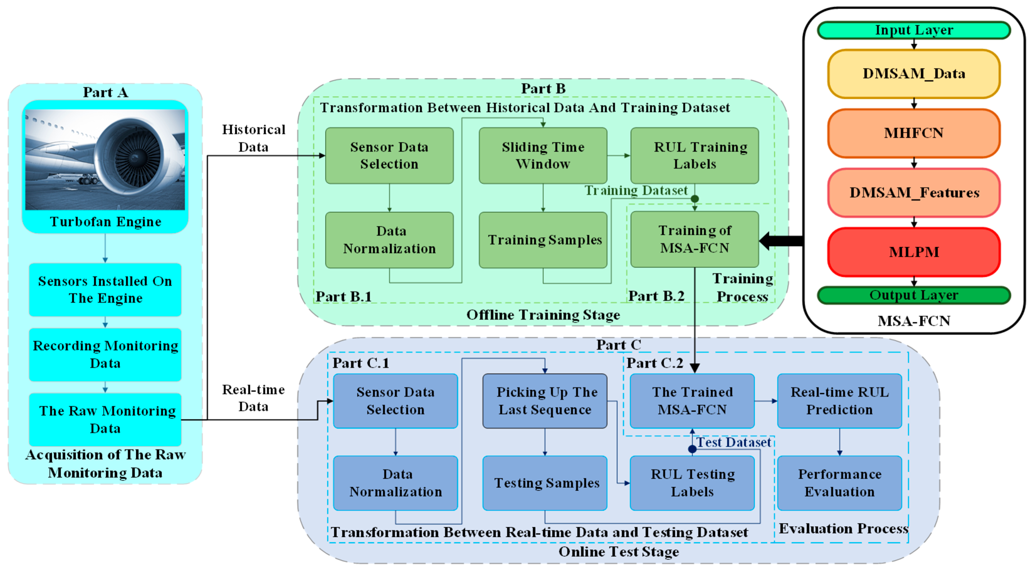
MSA-FCN consists of four modules, namely, the multi-head sensor data self-attention module (DMSAM_Data), the multi-head fully convolutional network (MHFCN), the multi-head spatial feature self-attention module (DMSAM_Features), and the multilayer perceptron module (MLPM), where the first three modules are constructed based on Transformer’s multi-head self-attention [22] and multi-head structure [22]. The first module DMSAM_Data and the third module DMSAM_Features form the aforementioned DMSAM. The overall structure of MSA-FCN and its key modules are shown in Figure 2.
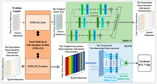
Figure 2.
MSA-FCN framework overview.
MSA-FCN extracts degraded representations with spatial characteristics from the input and weights the important data and representation parts for RUL by considering the correlation among various sensor data points and representations, thereby achieving the corresponding RUL prediction. The forward propagation of MSA-FCN is as follows: firstly, DMSAM_Data processes training sample, learns the correlation among different sensor data points, and assigns corresponding attention weights to the important parts of the above data for RUL. Then, MHFCN processes the weighted sensor data, focusing on the correlation among different sensor data points at the same time point through convolutional operations, thereby extracting the degradation representations with spatial characteristics. Subsequently, DMSAM_Features further processes the aforementioned representations, learns the correlation among these representations, and assigns corresponding attention weights to the key parts of the above representations for RUL. Finally, MLPM integrates the weighted representations with spatial characteristics and outputs the predicted RUL value. In more detail, the key modules of MSA-FCN are illustrated in the following sections.
3.2.1. Multi-Head Fully Convolutional Network (MHFCN)
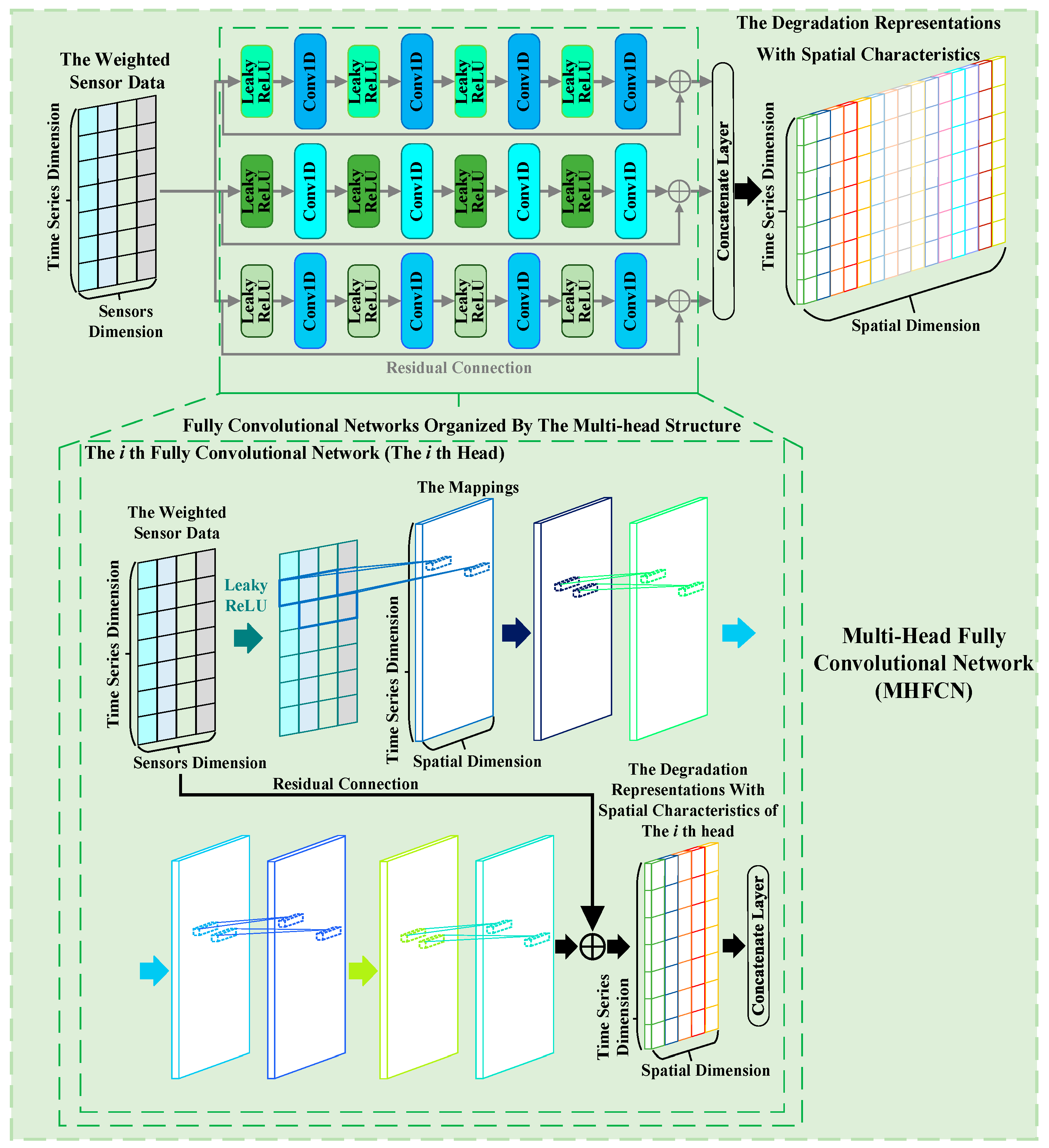
Within a piece of equipment, the degradation of one component not only causes the degradation of other components but also is affected by the degradation of other components. This degradation correlation among components implies that spatial characteristics are embedded in the corresponding sensor data. Therefore, MHFCN is constructed by integrating a fully convolutional network with a multi-head structure to take into account relevant spatial characteristics. As shown in Figure 3, MHFCN utilizes multiple fully convolutional networks to perform convolutional operations on the input in both the sensor and spatial dimensions, extracting the degradation representations with spatial characteristics from the sensor weighted data. Simultaneously, by organizing these fully convolutional networks in parallel through the multi-head structure, MHFCN can effectively enrich the representations it extracts, providing support for subsequent RUL prediction.
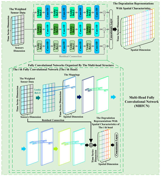
Figure 3.
Diagram of MHFCN.
The forward propagation of MHFCN is described as follows:
- (1)
- First, in each head, the mappings of the first layer are obtained by processing the weighted sensor data Bi along the sensor dimension. Each head of MHFCN (each fully convolutional network) uses convolutional kernels to perform convolution operations on multiple different sensor data points at each time point within the weighted data along the sensor dimension and traverses through the operation of sliding convolutional kernels, thereby obtaining the first layer mapping of the corresponding fully convolutional network. The steps above are shown in Equations (9) and (10).where , , , , , , and Y represent the weight of the th filter, the bias corresponding to Wi, the mapping of the th filter, the activation function, the convolution operation of the th filter, the number of the filters, and the mapping of Conv1D, respectively. It is worth noting that the aforementioned steps adopt the pre-activation function strategy [32], which helps capture the nonlinear relationships among different sensor data points and can enhance the modeling capabilities of MSA-FCN.
- (2)
- MHFCN performs three iterative processings of the data along the spatial dimension using Equations (9) and (10), thereby obtaining deep mappings on each head of MHFCN.
- (3)
- Each head of MHFCN combines the weighted data with the aforementioned mappings through residual connection [32] to extract the corresponding spatially characteristic degradation representations. Residual connection can reduce the training burden of neural networks and enhance the stability of MSA-FCN predictions for RUL. The calculation is shown in Equation (11).where and represent the mappings learned by the th head and the degradation representations with spatial features learned by the th head, respectively.
- (4)
- MHFCN uses a concatenation layer to aggregate the representations extracted from all its heads, thereby obtaining the final degradation representations with spatial characteristics . The calculation is shown in Equation (12).where represents number of the heads of MHFCN.
3.2.2. Dual Multi-Head Self-Attention Module (DMSAM)
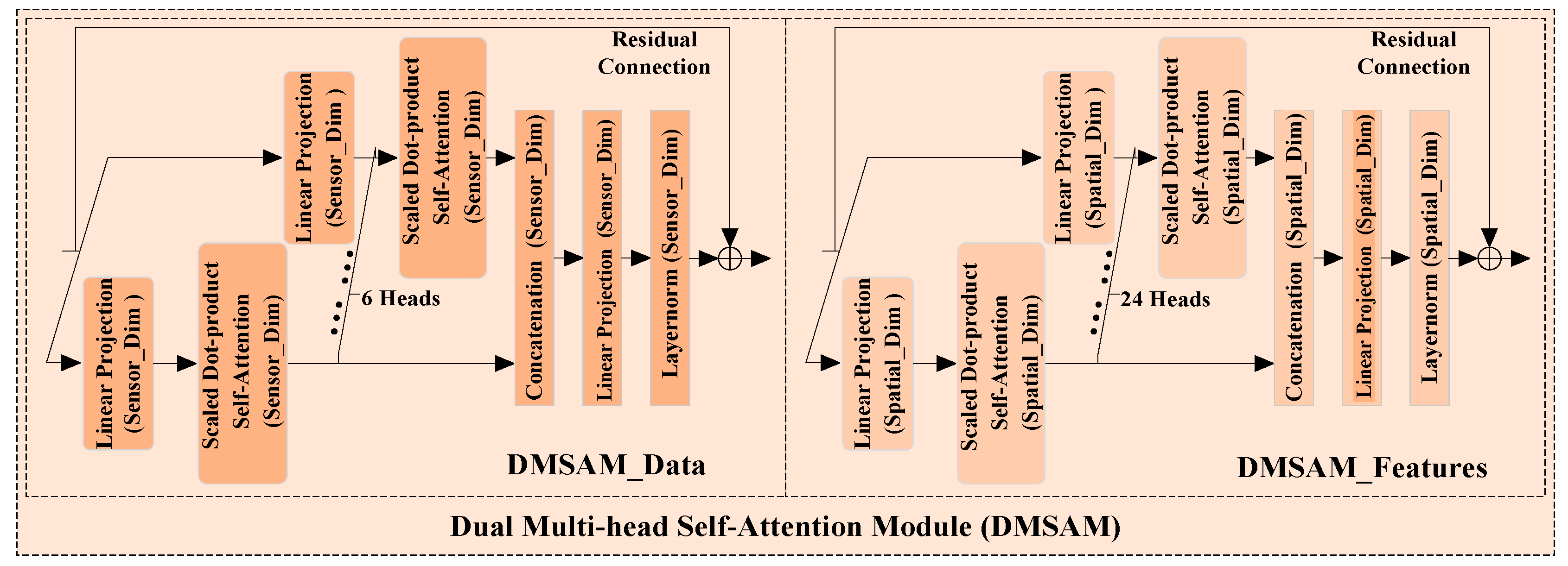
Importance differences in degradation information exist in both the sensor data and representations extracted by the deep neural network. However, some existing models for the RUL prediction of turbofan engines only consider the differences within the sensor data or within the extracted representations, which may result in the loss of some degradation information that can contribute significantly to the corresponding RUL prediction. To alleviate this challenge, DMSAM is built based on Transformer’s multi-head self-attention module. It aims to enhance the key parts of the data and representations that significantly contribute to RUL prediction by learning and allocating relevant attention weights, thus providing support for MSA-FCN’s RUL prediction. As shown in Figure 4, DMSAM consists of two modules, DMSAM_Data and DMSAM_Features, which process various sensor data points and representations extracted by MHFCN, respectively. Specifically, DMSAM_Data and DMSAM_Features process the input data and representations along the sensor and spatial dimensions, respectively, to learn the relationships between different data points and representations, dynamically compute relevant attention weights, and allocate those weights to the corresponding parts within them. Through the above processes, DMSAM_Data and DMSAM_Features can effectively generate weighted sensor data and weighted degradation representations with spatial characteristics, respectively. They share the same network structure, but the former uses more heads than the latter to adapt to the increased number of representations after MHFCN processing. The residual connection of both modules is performed after layer normalization, which is different from the residual connection in Transformer. This can be expressed as .
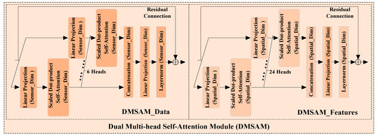
Figure 4.
Diagram of DMSAM.
DMSAM_Features and DMSAM_Data are identical in terms of the mechanism of data processing. Therefore, only the forward propagation of DMSAM_Features is described below.
- (1)
- DMSAM_Features has three computational steps in each of its heads (each spatial feature self-attention module).
- (1.1)
- Each head performs a linear projection of the degradation representations along the spatial dimension. This step is shown in Equation (1).
- (1.2)
- Each head applies a scaled dot-product self-attention mechanism in the spatial dimension to process the obtained query and key matrices, thereby learning the relationships among various representation parts. Based on these relationships, attention weights reflecting the importance of different representation parts are dynamically calculated and obtained. This step is shown in Equation (2).
- (1.3)
- Each head assigns the obtained attention weights to the corresponding representation parts. This step is shown in Equation (3).
- (2)
- DMSAM_Features utilizes a concatenation layer to aggregate the weighted degradation representations extracted from all its heads along the spatial dimension. This step is shown in Equation (4).
- (3)
- DMSAM_Features performs a linear projection on the aggregated output to ensure it maintains the same dimensions as along the spatial dimension. This step is shown in Equation (5).
- (4)
- DMSAM_Features combines the reshaped outputs and using a residual connection to extract the final weighted degradation representations with spatial characteristics .
3.2.3. Multilayer Perceptron Module (MLPM)
MLPM processes all degradation representations using a Multi-Layer Perceptron (MLP) [28,30] and outputs the corresponding RUL value. Firstly, MLPM utilizes a flattening layer to convert the degradation representations from a two-dimensional vector to a one-dimensional vector . Then, MLPM employs the MLP with two fully connected layers to process , integrating relevant representations. Finally, MLPM processes the integrated representations through a regression layer and outputs the predicted RUL value. The above computational steps are represented by Equations (13)–(16).
where , , , , , , and represent the weights of the first layer of the MLP, the bias corresponding to , the mapping of the first layer of the MLP, the weights of the second layer of the MLP, the bias corresponding to , the activation function, and the flattening layer, respectively. , , and represent the weights of the regression layer, the bias corresponding to , and the predicted RUL value, respectively.
3.3. Training of MSA-FCN and RUL Prediction Procedure
In this paper, MSA-FCN is trained using the Huber loss function [34]. This function is a piecewise loss function used for data-driven prediction tasks. By combining the characteristics of the Mean Absolute Error Loss (MAE Loss) and the Mean Squared Error Loss (MSE Loss), it can stably handle outliers in predicted and labeled values. It possesses a fast gradient descent speed and an appropriate gradient descent magnitude. The Huber loss function used is shown in Equations (17) and (18).
where the first and second terms in Equation (17) denote the Huber loss and L2 regularization, respectively. Meanwhile, , , and in Equation (17) denote the set of the trainable parameters, the set of the weights, and the penalty term, respectively. is an adjustable hyperparameter in Equation (18). When tends to zero, the loss function will approximate MAE Loss; when tends to infinity, the loss function will approximate MSE Loss. in Equation (18) is the number of training samples. Ultimately, the network parameters are updated, and the loss is minimized through the Adam optimizer and the back propagation algorithm. The training process of MSA-FCN is summarized by Algorithm 1.
| Algorithm 1: Training of MSA-FCN |
| Input: Training datasets , hyperparameters of the network. Output: The trained MSA-FCN with the optimized trainable parameters. 1: Repeat: 2: Sample a batch of data from Training datasets. 3: Use DMSAM_Data to process through Equations (1)–(5) and . 4: Use MHFCN to process through Equations (9)–(12). 5: Use DMSAM_Features to process through Equations (1)–(5) and . 6: Use MLPM to process for outputting the predicted through flatten operation and Equations (13)–(16). 7: Use the predicted and the corresponding training label to calculate the loss function through Equations (17) and (18). 8: Update the trainable parameters and minimize the loss function through the Adam optimizer and the back propagation algorithm. 9: Until convergence of the Huber loss. |
In this section, the RUL prediction procedure of the equipment is summarized. As shown in Figure 5, the procedure mainly contains three parts, i.e., the acquisition of the raw monitoring data (Part A), the offline training stage (Part B), and the online test stage (Part C).
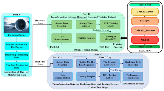
Figure 5.
Flowchart of the RUL prediction procedure using MSA-FCN.
- Part A
- Acquisition of the raw monitoring data.
- (a).
- The sensors are mounted on the corresponding components of the equipment.
- (b).
- The data reflecting the evolution of the components throughout their life cycles are recorded.
- (c).
- The raw monitoring data containing historical data and real-time data are obtained.
- Part B
- Offline training stage.
- Part B.1
- Transformation between historical data and training datasets.
- (a).
- The sensor data that have a definite change trend along the time series are selected from the historical data.
- (b).
- The selected sensor data are normalized.
- (c).
- A sliding time window operation is used to generate training samples from the normalized data, and a piece-wise function is utilized to generate the corresponding RUL training labels.
- (d).
- The samples and the labels are integrated to form training datasets.
- Part B.2
- Training process.
- (a).
- The proposed network of learning the degradation information are built to establish the proposed neural network.
- (b).
- Training datasets and Algorithm 1 are adopted to train the proposed neural network.
- (c).
- The trained neural network is sent to the online test stage.
- Part C
- Online test stage.
- Part C.1
- Transformation between real-time data and testing datasets.
- (a).
- The sensor data that have a definite change trend along the time series are selected from the real-time data.
- (b).
- The selected sensor data are normalized.
- (c).
- Testing samples and the corresponding RUL testing labels are generated by picking up the last sequence of each engine of the normalized data.
- (d).
- The samples and the labels are integrated to form testing datasets.
- Part C.2
- Evaluation process.
- (a).
- The testing datasets are fed into the trained neural network to predict the real-time RUL of the equipment.
- (b).
- The predicted RUL values and the RUL testing labels are used to calculate the experimental metrics.
- (c).
- The calculated metrics are employed to evaluate the performance of the proposed neural network.
4. RUL Prediction Experiment
4.1. Data Description
The Commercial Modular Aero-Propulsion System Simulation (C-MAPSS) turbofan engine dataset [35] is specifically designed to evaluate models for predicting the performance degradation and RUL of turbofan engines. This dataset collects data by simulating the degradation process of commercial turbofan engines under various operating conditions and failure modes, aiming to provide a comprehensive and realistic platform that assists researchers in accurately understanding and simulating engine behavior during actual operation. The C-MAPSS dataset utilizes advanced simulation techniques to mimic the performance degradation of turbofan engines. During the simulation, various operating conditions are adjusted, and multiple failure modes, such as turbine blade wear and sensor failures, are introduced to simulate different scenarios that an engine may encounter in real-world operation. The data are collected over multiple flight cycles, with each cycle fully simulating every stage from takeoff to landing, including takeoff, climb, cruise, descent, and landing.
To reflect the complexity of turbofan engines in real-world operation, the following operating conditions were simulated during the data acquisition process:
- (i)
- Different flight stages: The dataset covers all stages of flight, and the operating parameters such as thrust, airflow, temperature, and pressure for each stage were adjusted based on actual conditions.
- (ii)
- Environmental variables: Different environmental conditions, such as atmospheric temperature, humidity, and flight altitude, were also considered during the simulation to explore the potential impact of these external factors on engine performance.
- (iii)
- Failure modes and operational settings: Additionally, various failure modes were deliberately introduced into the simulation, and engine performance data under these failure modes were recorded. Meanwhile, different pilot operational settings, such as throttle position and flight speed, were also taken into account to enable a more comprehensive analysis of the impact of various factors on engine performance and degradation.
The C-MAPSS dataset consists of raw monitoring data generated by multiple sensor signals, which meticulously documents the performance changes in turbofan engines. The raw data include readings from 21 sensors, capturing various critical physical indicators that change over time, such as pressure, temperature, and rotational speed. In this paper, in order to investigate RUL prediction models in the situation of multiple operational conditions and fault modes, FD002 and FD004 of the C-MAPSS dataset are utilized to evaluate the performance of MSA-FCN. Both FD002 and FD004 contain corresponding historical datasets (for training) and real-time datasets (for testing), and information about both can be found in Table 1.

Table 1.
Summary of FD002 and FD004.
4.2. Data Preprocessing
4.2.1. Training Datasets
First, sensor data selection refers to the selection of historical sensor data. Not all sensor data in the dataset are utilized as training and testing samples. Actually, there are some sensor data that do not change significantly with the time series or even remain constant. These data are hardly helpful for predicting RUL and should be removed during sensor data selection. Referring to studies [28,30], 14 sensor data points of FD002 and FD004, i.e., sensor data numbered 2, 3, 4, 7, 8, 9, 11, 12, 13, 14, 15, 17, 20, and 21, are selected to generate training and testing samples for RUL prediction. The selected sensor data are summarized in Table 2.
Table 2.
Summary of the selected sensor data.
Then, data normalization is used to process the selected sensor data. Commonly, data in a small range have stronger sensitivity, which helps to accelerate the training process and enhance the perception of the data by the neural network. Therefore, it is necessary to use data normalization to limit the range of the data. The data to be processed are expressed as Equation (19).
where , , , and represent the th sensor data, the th time step data point in the th sensor data, the length of the time series, and the number of sensors, respectively. This paper adopts the min–max scaler to normalize each data point to the range of , which can be calculated by Equation (20).
where , , , , and represent the normalized data point, the minimum data point in the th sensor data, the maximum data point in the th sensor data, the lower bound of the range, and the upper bound of the range, respectively. After the normalization, all normalized data points can be expressed as Equation (21).
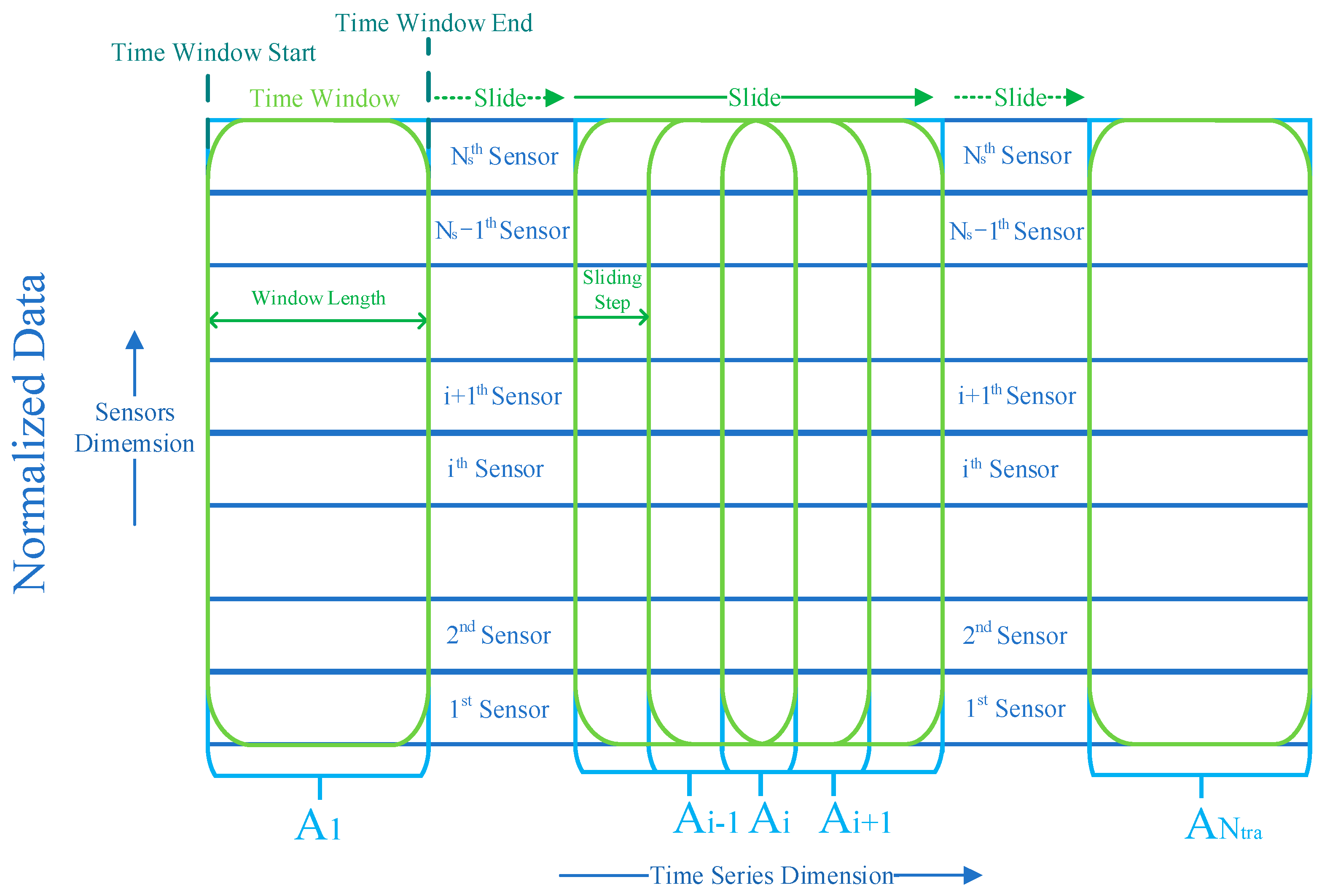
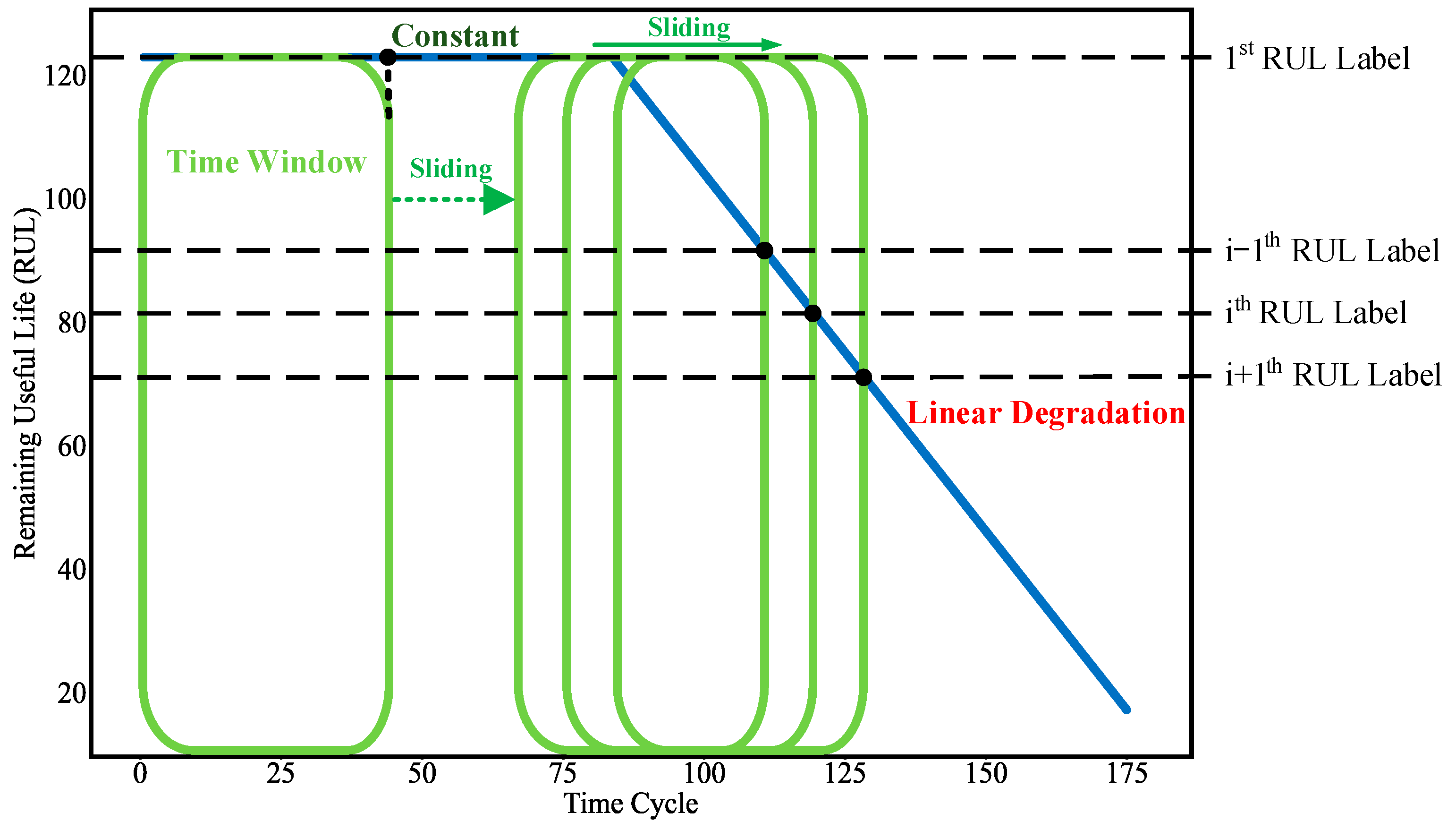
After that, as shown in Figure 6, a sliding time window operation [22,24,33] is used to process the normalized data. There are temporal dependencies among data points of the normalized data. Therefore, it is vital to capture these dependencies, and the sliding time window operation is utilized to accomplish this task. The th sample obtained by the operation can be expressed as Equation (22).
where , , and represent the start of the time window, the end of the time window, and the length of the time window, respectively. Sliding step is set to 1 to obtain more samples for training. After sliding the time window of a sliding step, the th sample can be expressed as Equation (23).
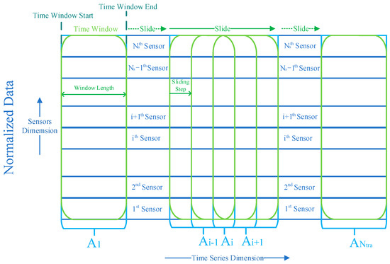
Figure 6.
Diagram of the sliding time window operation.
The number of the samples obtained by the operation can be calculated by Equation (24).
The th training sample is exactly the th sample obtained by the operation. Finally, all training samples are generated by performing the sliding time window operation on the normalized data.
In the end, as shown in Figure 7, a piecewise function [36] is used to generate the RUL labels of the training samples. The function is made of two parts, namely, a constant part and a linear degradation part. The constant part means that the state of the equipment is healthy, while the linear degradation part indicates that the equipment is in a continuous degradation process until failures occur. The RUL label of each training sample is the RUL value at the end of the time window.
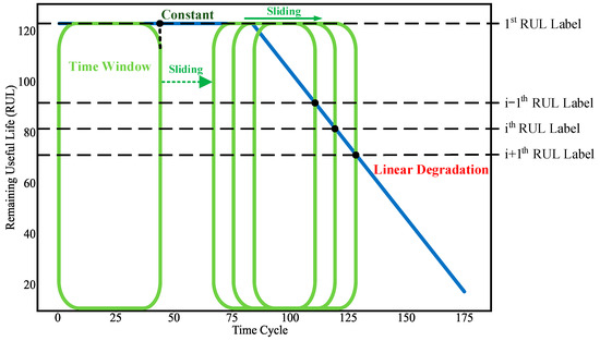
Figure 7.
Diagram showing the generation of RUL labels using the piecewise function.
4.2.2. Testing Datasets
The generation of testing datasets is identical to the generation of training datasets in terms of sensor data selection and data normalization, as mentioned above. The difference is that the final generation of the testing datasets is performed by picking up the last sequence of each engine of the transformed real-time data to obtain the corresponding testing samples and corresponding RUL labels .
4.3. Experimental Setup
All experiments were performed on a laptop computer equipped with AMD Ryzen 7 5800H CPU (AMD, Sunnyvale, CA, USA), 16-GB RAM, and GeForce RTX 3070 Laptop GPU (Nvidia, Santa Clara, CA, USA). A software environment with Keras 2.6.0 based on Tensorflow 2.6.0 and Python 3.9.0 was used.
The model parameters of MSA-FCN are summarized in Table 3. These parameters were tuned by grid search. The training epoch was set to 180, and the batch size was set to 512. The initial RUL value was set to 125. The window lengths of the sliding time window operation were set to 20 and 18 on FD002 and FD004, respectively. The Adam algorithm was used as the optimizer to minimize the loss function, and the learning rate was set to 0.0005. is an adjustable hyperparameter in the loss function, and was set to 1 for Huber loss. for L2 regularization was set to 0.001.
Table 3.
Summary of MSA-FCN’s model parameters.
4.4. Experimental Metrics
In this paper, both the Root Mean Squared Error (RMSE) and Score (referenced as [35]) are used as performance metrics to evaluate the performance of MSA-FCN.
RMSE reflects the accuracy of the RUL prediction model. Therefore, the corresponding model should aim to achieve as low RMSE values as possible. RMSE can be represented by Equation (25).
where , , and represent the number of the testing samples, the predicted RUL of the th testing sample, and the RUL label of the th testing sample, respectively.
The Score Function [35] is used in RUL prediction to evaluate the timeliness of model predictions. When the model’s predicted RUL lags behind the actual RUL, such prediction lags may cause potential engine failures to be overlooked, which can lead to serious related accidents. The Score Function processes prediction lags through a penalty mechanism, assigning a higher Score to relevant predictions. Specifically, the Score Function captures any deviation between the predicted RUL and the actual value, assigning a corresponding penalty coefficient based on the degree of deviation. When the predicted value lags behind the actual value, the penalty coefficient increases, resulting in a relatively higher Score. Conversely, when the predicted value is ahead of or equal to the actual value, the penalty coefficient is smaller, resulting in a relatively lower Score. Therefore, to improve the timeliness of RUL predictions, prediction models should strive to achieve the lowest possible Score. The Score Function and Score can be calculated using Equation (26) and Equation (27), respectively.
To reduce randomness during training and verify the stability of MSA-FCN, the results reported in subsequent sections are based on the mean (mean) and standard deviation (STD) of ten independent experiments.
In addition, Equation (28) is used in this paper to calculate the numerical reduction range of each performance metric.
4.5. Experimental Results
Table 4 shows the computational cost and number of training parameters required to conduct experiments with MSA-FCN on FD002 and FD004, respectively.
Table 4.
Computational cost and number of trainable parameters.
Table 5 presents the results of the RUL prediction performance metrics for MSA-FCN on the FD002 and FD004 datasets. Clearly, MSA-FCN performs better in RUL prediction on FD002 compared with FD004. This difference may stem from the varying number of failure modes contained in the two datasets. FD004 includes two failure modes, while FD002 has only one. Generally speaking, datasets with multiple failure modes pose greater challenges to RUL prediction models.
Table 5.
Experimental results of MSA-FCN on RMSE and Score.
Figure 8a,b respectively showcase the RUL prediction results of MSA-FCN for all engines in the FD002 and FD004 datasets. The horizontal axis represents engine codes, while the vertical axis denotes RUL values. Overall, the RUL curves predicted by MSA-FCN (orange) closely align with the actual RUL curves (blue). Specifically, the RUL curves in Figure 8a are more tightly clustered than those in Figure 8b, further verifying the difference in prediction performance of MSA-FCN across the two datasets.
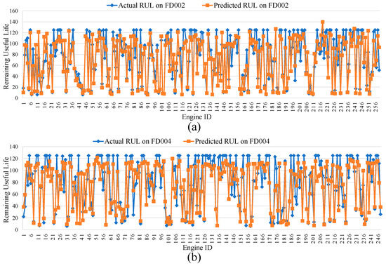
Figure 8.
RUL prediction results for the tested engines: (a) FD002 Engines and (b) FD004 Engines.
Table 6 and Figure 9a–f exhibit the RUL prediction results of MSA-FCN for six test engines (numbered #45, #177, #236, #8, #135, and #216) from the FD002 and FD004 datasets. According to the table, despite slight lags in the predictions for #236, #8, and #135, the RUL values predicted by MSA-FCN are generally close to the actual RUL values. From the figures, it is evident that the RUL curves predicted by MSA-FCN (blue) closely follow the actual RUL curves (green), and these curves nearly overlap during the linear degradation phase of the engines.
Table 6.
RUL prediction results for the six different tested engines from FD002 and FD004.
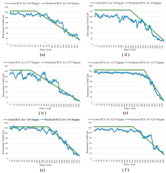
Figure 9.
RUL prediction results for different tested engines. (a) Test engine #45 from FD002; (b) test engine #177 from FD002; (c) test engine #236 from FD002; (d) test engine #8 from FD004; (e) test engine #135 from FD004; and (f) test engine #216 from FD004.
In conclusion, these results fully demonstrate the effectiveness of MSA-FCN in predicting RUL values for turbofan engines.
5. Performance Comparison and Discussion
5.1. Comparison with Other Models
In this section, MSA-FCN is compared with 11 existing deep neural networks for the RUL prediction of turbofan engines, including DSCN [30], MS-DCNN [26], LTSM-Attention [27], AGCNN [28], LSTM-INIFR [25], MCLSTM [29], Bi-level LSTM Scheme [24], LSTM Model [37], SMDN [38], BiGRU-TSAM [39], and IDMFFN [40]. The experimental results are summarized in Table 7 where N/A represents results that are not reported in the corresponding paper; underlined values indicate sub-optimal results; and bold values represent the optimal results. It should be noted that the experimental results of MSA-FCN in Section 4.5 are presented in this section with two decimal places kept for comparison with the other networks.
Table 7.
Performance comparison of MSA-FCN with other deep neural networks.
Overall, MSA-FCN performs best on all performance metrics for both the FD002 and FD004 datasets. Specifically, compared with the sub-optimal results, MSA-FCN achieves a reduction of 3.10% and 6.45% in RMSE and Score, respectively, on the FD002 dataset. On the FD004 dataset, it attains a decrease of 5.04% and 28.11% in RMSE and Score, respectively. We additionally calculated the sum (sum) and average (average) of RMSE and Score across all networks. Compared with the sub-optimal outcomes, MSA-FCN reduces both the sum and average of RMSE by 4.14% and lowers the sum and average of Score by 23.61%. These results indicate that, compared with the other 11 approaches, MSA-FCN can achieve more accurate and timely RUL prediction, demonstrating superior overall prediction performance.
Table 8 demonstrates a comparison of the robustness of MSA-FCN and the other models in RUL prediction. As shown in the table, MSA-FCN achieved the best results in all Score STDs, and it obtained the second-best results in all RMSE STDs. Overall, compared with the other models, MSA-FCN exhibits superior stability and robustness in multiple experimental tests, both in terms of prediction accuracy and timeliness.
Table 8.
Robustness comparison of MSA-FCN with the other deep neural networks.
Table 9 compares the computational cost of training among MSA-FCN and the other models. As shown in the table, MSA-FCN does not achieve the minimum training time per epoch. Therefore, compared with other models, MSA-FCN does not have a significant advantage in terms of computational cost for RUL prediction, which will be a focus of improvement in future research work.
Table 9.
Computational cost comparison of MSA-FCN with the other deep neural networks.
In summary, compared with some of the existing deep neural networks used for predicting the RUL of turbofan engines, MSA-FCN can achieve competitive advantages in terms of accuracy and timeliness. However, it does not yet exhibit outstanding performance in robustness and computational cost. Therefore, one of focuses of our future research work is to achieve a trade-off among performance, stability, and computational time for the prediction model.
5.2. Ablation Experiments for MHFCN and DMSAM
This section explores the critical roles of MHFCN and DMSAM in the prediction performance of MSA-FCN through four sets of ablation experiments conducted on the FD002 and FD004 datasets. The neural networks involved in the experiments include MSA-FCN, a neural network without DMSAM_Data (W/O DMSAM_1), a neural network without DMSAM_Features (W/O DMSAM_2), a neural network without the entire DMSAM (W/O DMSAM), and a neural network without MHFCN (W/O MHFCN). All experimental results are detailed in Table 10.
Table 10.
Impact of MHFCN and DMSAM on the prediction performance of MSA-FCN.
It can be observed that MSA-FCN significantly outperforms the other four variant neural networks in terms of the average RMSE and Score across all tested datasets. This result confirms that MHFCN and DMSAM (including DMSAM_Data and DMSAM_Features) can capture and emphasize key parts within the sensor data and degradation representations with spatial characteristics, thereby improving RUL prediction performance of MSA-FCN.
Notably, W/O DMSAM exhibits the highest average values for both RMSE and Score. This phenomenon reveals that the lack of effective enhancement of key degradation information can severely compromise accuracy of RUL predictions. Similarly, it is worth noting that W/O MHFCN also shows a decline in performance compared with MSA-FCN in terms of RMSE and Score. This result suggests that neglecting the spatial characteristics hidden within the monitoring data may lead to an insufficient understanding of the equipment degradation mechanism, further affecting accuracy of RUL predictions.
Additionally, W/O DMSAM_1 and W/O DMSAM_2 demonstrate moderate performance across all tested datasets. This may be due to their ability to capture and enhance only partial key information, thus preventing further optimization of RUL prediction performance.
5.3. Ablation Experiments for Residual Connections within DMSAM
This section explores the impact of residual connections within DMSAM on the prediction performance of MSA-FCN. Four sets of ablation experiments were conducted on the FD002 and FD004 datasets. The neural networks involved in the experiments include the following: MSA-FCN with full dual residual connections, a neural network adopting the original Transformer residual connection (TFormer Connection), a neural network with only the residual connection within DMSAM_Data (Connect_1), a neural network with only the residual connection within DMSAM_Features (Connection_2), and a neural network without any residual connections within DMSAM (W/O Connection). The relevant experimental results are summarized in Table 11.
Table 11.
Impact of residual connections within DMSAM on the prediction performance of MSA-FCN.
Firstly, although the average RMSE of TFormer Connection on FD004 is slightly lower than that of MSA-FCN, the average RMSE of MSA-FCN on FD002 is the smallest among all variant neural networks. Secondly, despite MSA-FCN having a slightly higher average Score on FD002 compared with Connect_2, its average Score on FD004 is the lowest among all variant neural networks. Finally, MSA-FCN has the lowest STD values among all variant neural networks across all metrics.
The partial improvement in MSA-FCN’s prediction performance due to the residual connections within DMSAM can be attributed to the dual residual connections effectively alleviating the training burden of the network. This accelerates the decrease in loss during the training process and effectively avoids the problem of gradient vanishing. These experimental results can provide new insights for further optimizing neural network structures and improving RUL prediction performance.
5.4. Ablation Experiments for the Multi-Head Structure
This section validates the impact of the multi-head structure on the RUL prediction performance of MSA-FCN by conducting relevant ablation experiments on the FD002 and FD004 datasets. To this end, seven comparative models were designed for RUL prediction, namely, SSD-SHF-SSF, SSD-SHF-MSF, SSD-MHF-SSF, MSD-SHF-SSF, MSD-MHF-SSF, MSD-SHF-MSF, and SSD-MHF-MSF. Herein, SSD, SHF, and SSF represent the Single-head Sensor Data Self-Attention Module, the Single-head Fully Convolutional Neural Module, and the Single-head Spatial Feature Self-Attention Module, respectively. MSD, MHF, and MSF stand for DMSAM_Data, MHFCN, and DMSAM_Features, respectively. The performance metric results for all models are summarized in Table 12.
Table 12.
The influence of the corresponding neural network established by adopting the multi-head structure on the prediction performance.
In terms of RMSE and Score, MSA-FCN achieves lower average values compared with SSD-SHF-SSF, which can be regarded as a completely single-head structured neural network. Specifically, on FD002, the average values of MSA-FCN are reduced by 8.28% and 58.60% for RMSE and Score, respectively, compared with SSD-SHF-SSF. On FD004, the reductions are even greater, at 15.30% and 76.38%, respectively. These results indicate that when processing datasets containing multiple failure modes, the multi-head structure enables MSA-FCN to extract useful degradation representations from raw monitoring data, thereby effectively improving the accuracy of RUL prediction.
Except for the Score average on FD002, the remaining averages achieved by MSA-FCN are the lowest among all comparison models. This result suggests that DMSAM_Data, MHFCN, and DMSAM_Features, constructed using the multi-head structure, enable MSA-FCN to enrich the extracted representations, leading to more timely RUL predictions. Finally, the STD values obtained by MSA-FCN are the lowest among all the comparison models, indicating that the multi-head structure enhances the stability of its RUL prediction results.
In summary, the multi-head structure allows MSA-FCN to focus on multiple aspects of raw monitoring data including different degradation trends, stages, and interactions among components. Therefore, MSA-FCN, based on the multi-head structure, can achieve more accurate, timely, and stable results in RUL prediction.
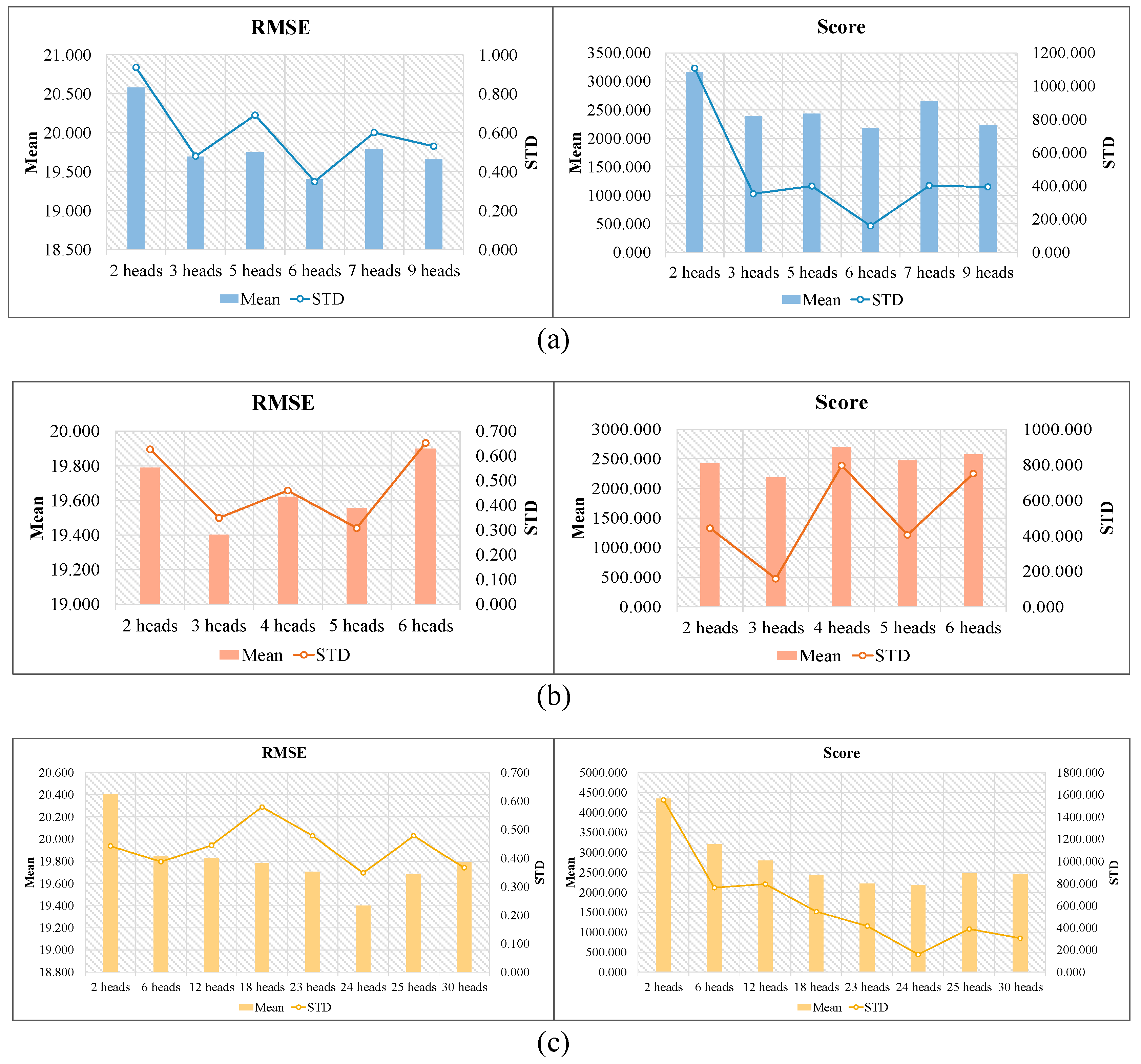
In this section, this paper also investigates the influences of heads of the multi-head structure on RUL prediction performance on FD004. Table 13, Table 14 and Table 15 summarize the experimental results for the three modules (DMSAM_Data, MHFCN, and DMSAM_Features) using different numbers of heads, respectively. Figure 10a–c are also used to further illustrate the experimental results. As can be seen from the above tables and figures, to achieve the lowest mean values on both RMSE and Score, the optimal number of heads for each model is as follows: DMSAM_Data uses 6 heads, MHFCN uses 3 heads, and DMSAM_Features uses 24 heads. It can be observed that the three modules using fewer heads obtain higher mean values in terms of RMSE and Score, while the three modules using more heads only slightly improve the corresponding performance metrics, or even make them worse. Based on these observations, it can be concluded that insufficient learning of the degradation information, due to the use of fewer heads and the over-parameterization of the neural network, due to the use of more heads, may lead to poor performance in RUL prediction. Therefore, it is crucial that a balance between performance and computation cost is found for RUL prediction.
Table 13.
Effect of the number of heads in DMSAM_Data on the performance of RUL prediction.
Table 14.
Effect of the number of heads in MHFCN on RUL prediction performance.
Table 15.
Effect of the number of heads in DMSAM_Features on RUL prediction.
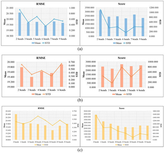
Figure 10.
Effects of the multi-head structure’s number of heads on RUL prediction: (a) DMSAM_Data; (b) MHFCN; and (c) DMSAM_Features.
In summary, MSA-FCN designed by the multi-head structure can effectively and adequately focus on various aspects of the raw monitoring data including different degradation trends, degradation stages, and degradation rates. Therefore, the multi-head structure enables the neural network to achieve more accurate and robust RUL prediction results.
6. Conclusions
In this paper, a novel deep neural network, the multi-head self-attention-based fully convolutional network (MSA-FCN), is proposed to predict the RUL of turbofan engines. MSA-FCN not only focuses on the degradation correlation among various components within the engine but also considers the differences in importance of various sensor data points and degradation representations for RUL prediction. Based on these features, MSA-FCN can extract valuable and abundant degradation representations under multiple operating conditions and failure modes, thus achieving RUL prediction for the corresponding turbofan engines. The experimental results using the C-MAPSS dataset demonstrate that MSA-FCN possesses competitive advantages in terms of accuracy and timeliness for RUL prediction when compared with 11 existing deep neural networks.
In the future, the authors will focus on a knowledge-based and data-driven RUL prediction method to achieve better prediction performance with fewer training samples while further enhancing the generalization capability and transferability of our RUL prediction method.
Author Contributions
Methodology, Z.L.; writing—original draft, Z.L.; software, Z.L.; data curation, Z.L.; conceptualization, X.Z., A.X., M.G. and A.J.; writing—review and editing, X.Z., A.X., M.G. and A.J. All authors have read and agreed to the published version of this manuscript.
Funding
This work was supported by the National Natural Science Foundation of China (Grant No. U22A2047), the Basic Public Welfare Research Project of Zhejiang Province (Grant No. LGG22F030005), and the “Ling-Yan” Research and Development Project of Zhejiang Province of China (Grant No. 2023C01157).
Data Availability Statement
The datasets are available from the corresponding author upon reasonable request.
Conflicts of Interest
The authors declare that they have no known competing financial interests or personal relationships that could have appeared to influence the work reported in this paper.
References
- Hu, C.; Jain, G.; Tamirisa, P.; Gorka, T. Method for predicting capacity and predicting remaining useful life of lithium-ion battery. Appl. Energy 2014, 126, 182–189. [Google Scholar] [CrossRef]
- Qian, Y.; Ya, R.; Gao, R.X. A multi-time scale approach to remaining useful life prediction in rolling bearing. Mech. Syst. Signal Process. 2017, 83, 549–567. [Google Scholar] [CrossRef]
- Thelen, A.; Li, M.; Hu, C.; Bekyarova, E.; Kalinin, S.; Sanghadasa, M. Augmented model-based framework for battery remaining useful life prediction. Appl. Energy 2022, 324, 119624. [Google Scholar] [CrossRef]
- Aye, S.; Heyns, P. An integrated Gaussian process regression for prediction of remaining useful life of slow speed bearings based on acoustic emission. Mech. Syst. Signal Process. 2017, 84, 485–498. [Google Scholar] [CrossRef]
- Benkedjouh, T.; Medjaher, K.; Zerhouni, N.; Rechak, S. Remaining useful life prediction based on nonlinear feature reduction and support vector regression. Eng. Appl. Artif. Intell. 2013, 26, 1751–1760. [Google Scholar] [CrossRef]
- Wu, D.; Jennings, C.; Terpenny, J.; Gao, R.X.; Kumara, S. A Comparative Study on Machine Learning Algorithms for Smart Manufacturing: Tool Car Prediction Using Random Forests. J. Manuf. Sci. Eng.-Trans. ASME 2017, 139, 071018. [Google Scholar] [CrossRef]
- Javed, K.; Gouriveau, R.; Zerhouni, N. A New Multivariate Approach for Prognostics Based on Extreme Learning Machine and Fuzzy Clustering. IEEE Trans. Cybern. 2015, 45, 2626–2639. [Google Scholar] [CrossRef] [PubMed]
- Yan, Y.; Luh, P.B.; Pattipati, K.R. Fault Prognosis of Key Components in HVAC Air-Handling Systems at Component and System Levels. IEEE Trans. Autom. Sci. Eng. 2020, 17, 2145–2153. [Google Scholar] [CrossRef]
- Ren, L.; Sun, Y.; Cui, J.; Zhang, L. Bearing remaining useful life prediction based on deep autoencoder and deep neural networks. J. Manuf. Syst. 2018, 48, 71–77. [Google Scholar] [CrossRef]
- Wu, Z.; Yu, S.; Zhu, X.; Ji, Y.; Pecht, M. A Weighted Deep Domain Adaptation Method for Industrial Fault Prognostics According to Prior Distribution of Complex Working Conditions. IEEE Access 2019, 7, 139802–139814. [Google Scholar] [CrossRef]
- Shi, J.; Rivera, A.; Wu, D. Battery health management using physics-informed machine learning: Online degradation modeling and remaining useful life prediction. Mech. Syst. Signal Process. 2022, 179, 109347. [Google Scholar] [CrossRef]
- Babu, G.S.; Zhao, P.; Li, X. Deep Convolutional Neural Network Based Regression Approach for Prediction of Remaining Useful Life. In Proceedings of the International Conference on Database Systems for Advanced Applications, Dallas, TX, USA, 16–19 April 2016; pp. 214–228. [Google Scholar]
- Xia, M.; Li, T.; Shu, T.; Wan, J.; de Silva, C.W.; Wang, Z. A Two-Stage Approach for the Remaining Useful Life Prediction of Bearings Using Deep Neural Networks. IEEE Trans. Ind. Inform. 2019, 15, 3703–3711. [Google Scholar] [CrossRef]
- Zheng, S.; Ristovski, K.; Farahat, A.; Gupta, C. Long Short-Term Memory Network for Remaining Useful Life prediction. In Proceedings of the 2017 IEEE International Conference on Prognostics and Health Management (ICPHM), Dallas, TX, USA, 19–21 June 2017; pp. 88–95. [Google Scholar]
- Deutsch, J.; He, D. Using Deep Learning-Based Approach to Predict Remaining Useful Life of Rotating Components. IEEE Trans. Syst. Man Cybern. Syst. 2018, 48, 11–20. [Google Scholar] [CrossRef]
- Behera, S.; Misra, R.; Sillitti, A. Multiscale deep bidirectional gated recurrent neural networks based prognostic method for complex non-linear degradation systems. Inform. Sci. 2021, 554, 120–144. [Google Scholar] [CrossRef]
- Han, T.; Wang, Z.; Meng, H. End-to-end capacity prediction of Lithium-ion batteries with an enhanced long short-term memory network considering domain adaptation. J. Power Sources 2022, 520, 230823. [Google Scholar] [CrossRef]
- Jayasinghe, L.; Samarasinghe, T.; Yuenv, C.; Low, J.C.N.; Ge, S.S. Temporal Convolutional Memory Networks for Remaining Useful Life Prediction of Industrial Machinery. In Proceedings of the 2019 IEEE International Conference on Industrial Technology (ICIT), Melbourne, Australia, 13–15 February 2019; pp. 915–920. [Google Scholar]
- Xia, T.; Song, Y.; Zheng, Y.; Pan, E.; Xi, L. An ensemble framework based on convolutional bi-directional LSTM with multiple time windows for remaining useful life prediction. Comput. Ind. 2019, 115, 103182. [Google Scholar] [CrossRef]
- Li, W.; Zhang, L.-C.; Wu, C.-H.; Wang, Y.; Cui, Z.-X.; Niu, C. A data-driven approach to RUL prediction of tools. Adv. Manuf. 2024, 12, 6–18. [Google Scholar] [CrossRef]
- Kim, G.; Choi, J.G.; Lim, S. Using transformer and a reweighting technique to develop a remaining useful life estimation method for turbofan engines. Eng. Appl. Artif. Intell. 2024, 133, 108475. [Google Scholar] [CrossRef]
- Vaswani, A.; Shazeer, N.; Parmar, N.; Uszkoreit, J.; Jones, L.; Gomez, A.N.; Kaiser, L.; Polosukhin, I. Attention is all you need. In Advances in Neural Information Processing Systems 30 (NIPS 2017); Curran Associates, Inc.: Red Hook, NY, USA, 2017; pp. 5998–6008. [Google Scholar]
- Zhou, K.; Tang, J. A wavelet neural network informed by time-domain signal preprocessing for bearing remaining useful life prediction. Appl. Math. Model. 2023, 122, 220–241. [Google Scholar] [CrossRef]
- Song, T.; Liu, C.; Wu, R.; Jin, Y.; Jiang, D. A hierarchical scheme for remaining useful life prediction with long short-term memory networks. Neurocomputing 2022, 487, 22–33. [Google Scholar] [CrossRef]
- Xiao, L.; Tang, J.; Zhang, X.; Bechhoefer, E.; Ding, S. Remaining useful life prediction based on intentional noise injection and feature reconstruction. Reliab. Eng. Syst. Saf. 2021, 215, 107871. [Google Scholar] [CrossRef]
- Li, H.; Zhao, W.; Zhang, Y.; Zio, E. Remaining useful life prediction using multi-scale deep convolutional neural network. Appl. Soft Comput. 2020, 89, 106113. [Google Scholar] [CrossRef]
- Chen, Z.; Wu, M.; Zhao, R.; Guretno, F.; Yan, R.; Li, X. Machine Remaining Useful Life Prediction via an Attention-Based Deep Learning Approach. IEEE Trans. Ind. Electron. 2021, 68, 2521–2531. [Google Scholar] [CrossRef]
- Liu, H.; Liu, Z.; Jia, W.; Lin, X. Remaining Useful Life Prediction Using a Novel Feature-Attention-Based End-to-End Approach. IEEE Trans. Ind. Inform. 2021, 17, 1197–1207. [Google Scholar] [CrossRef]
- Xiang, S.; Qin, Y.; Luo, J.; Pu, H.; Tang, B. Multicellular LSTM-based deep learning model for aero-engine remaining useful life prediction. Reliab. Eng. Syst. Saf. 2021, 216, 107927. [Google Scholar] [CrossRef]
- Wang, B.; Lei, Y.; Li, N.; Yan, T. Deep separable convolutional network for remaining useful life prediction of machinery. Mech. Syst. Signal Process. 2019, 134, 106330. [Google Scholar] [CrossRef]
- Fan, L.; Chai, Y.; Chen, X. Trend attention fully convolutional network for remaining useful life prediction. Reliab. Eng. Syst. Saf. 2022, 225, 108590. [Google Scholar] [CrossRef]
- He, K.; Zhang, X.; Ren, S.; Sun, J. Identity Mappings in Deep Residual Networks. In Computer Vision—ECCV 2016, 14th European Conference on Computer Vision, Amsterdam, The Netherlands, 11–14 October 2016; Springer: Cham, Switzerland, 2016; pp. 630–645. [Google Scholar]
- Ba, J.L.; Kiros, J.R.; Hinton, G.E. Layer Normalization. arXiv 2016, arXiv:1607.06450. [Google Scholar]
- Huber, P.J. Robust Estimation of a Location Parameter. Ann. Math. Stat. 1964, 35, 73–101. [Google Scholar] [CrossRef]
- Saxena, A.; Goebel, K.; Simon, D.; Eklund, N. Damage propagation modeling for aircraft engine run-to-failure simulation. In Proceedings of the 2008 International Conference on Prognostics and Health Management, Denver, CO, USA, 6–9 October 2008; pp. 1–9. [Google Scholar] [CrossRef]
- Heimes, F.O. Recurrent neural networks for remaining useful life estimation. In Proceedings of the 2008 International Conference on Prognostics and Health Management, Denver, CO, USA, 6–9 October 2008; pp. 1–6. [Google Scholar] [CrossRef]
- Ruan, D.; Wu, Y.; Yan, J. Remaining Useful Life Prediction for Aero-Engine Based on LSTM and CNN. In Proceedings of the 2021 33rd Chinese Control and Decision Conference (CCDC), Kunming, China, 22–24 May 2021; pp. 6706–6712. [Google Scholar]
- Xiang, S.; Qin, Y.; Luo, J.; Pu, H. Spatiotemporally Multidifferential Processing Deep Neural Network and its Application to Equipment Remaining Useful Life Prediction. IEEE Trans. Ind. Inform. 2022, 18, 7230–7239. [Google Scholar] [CrossRef]
- Zhang, J.; Jiang, Y.; Wu, S.; Li, X.; Luo, H.; Yin, S. Prediction of remaining useful life based on bidirectional gated recurrent unit with temporal self-attention mechanism. Reliab. Eng. Syst. Saf. 2022, 221, 108297. [Google Scholar] [CrossRef]
- Li, X.; Jiang, H.; Liu, Y.; Wang, T.; Li, Z. An integrated deep multiscale feature fusion network for aeroengine remaining useful life prediction with multisensor data. Knowl.-Based Syst. 2022, 235, 107652. [Google Scholar] [CrossRef]


Disclaimer/Publisher’s Note: The statements, opinions and data contained in all publications are solely those of the individual author(s) and contributor(s) and not of MDPI and/or the editor(s). MDPI and/or the editor(s) disclaim responsibility for any injury to people or property resulting from any ideas, methods, instructions or products referred to in the content. |
© 2024 by the authors. Licensee MDPI, Basel, Switzerland. This article is an open access article distributed under the terms and conditions of the Creative Commons Attribution (CC BY) license (https://creativecommons.org/licenses/by/4.0/).