
A Swarm Intelligence Solution for the Multi-Vehicle Profitable Pickup and Delivery Problem


Abstract
:1. Introduction
2. Related Studies
3. Problem Definition
- The pairing constraint stipulates that a predefined customer pair is assigned to each request (pickup and delivery).
- Precedence constraint: Priority must be given to visiting the pickup customer over the delivery customer.
- The time limit for journeys: Every vehicle is subject to a daily travel time restriction that must not be surpassed during the service of customers.
- Every vehicle should depart from and arrive at the depot with an empty load.
- A single visit is permitted per customer.
4. Proposed Method
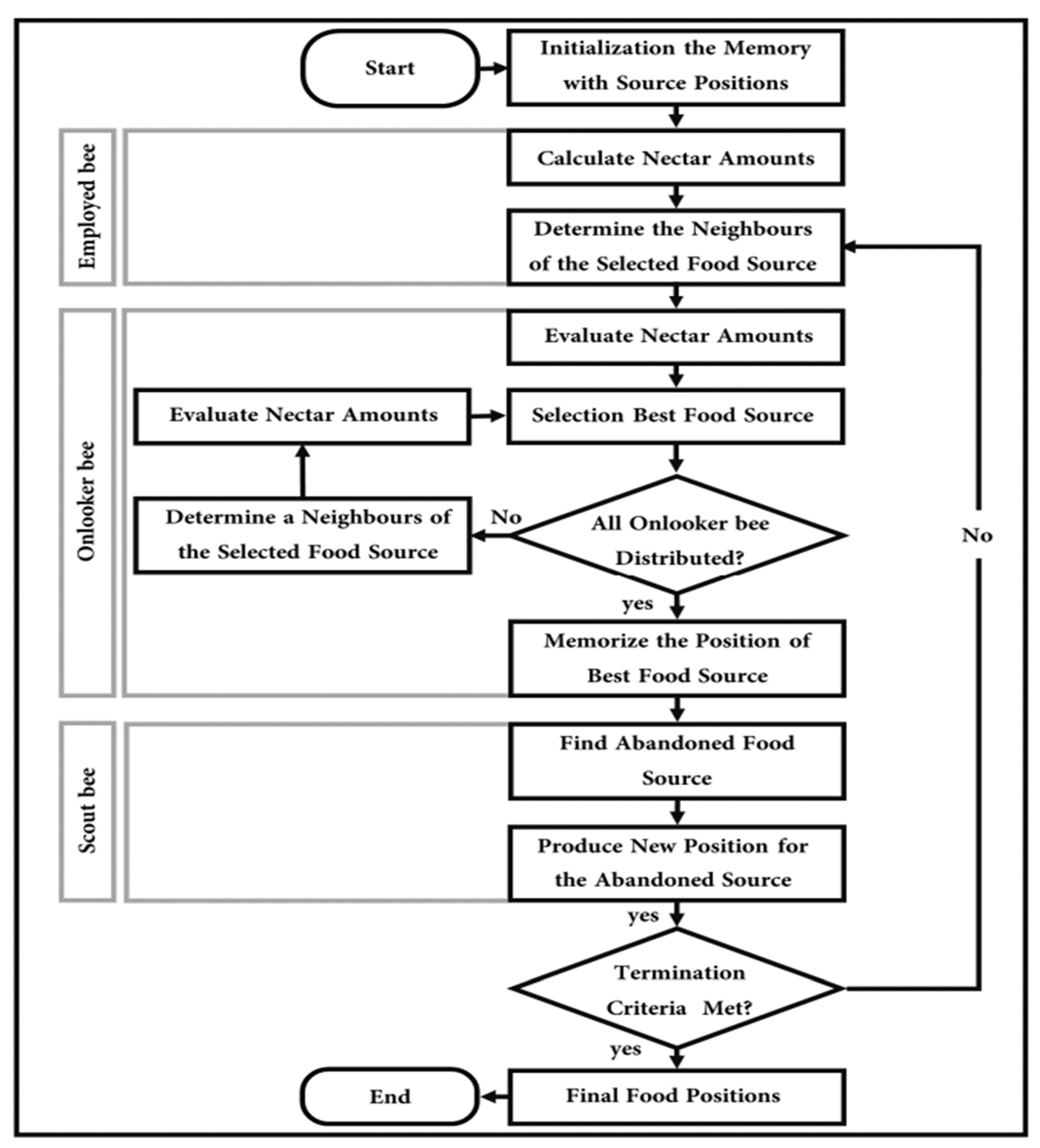
4.1. ABC without Clustering (ABC)
- Employed bee phase:
- Relocate a pickup customer only: Choose one pickup customer randomly and relocate its position, such that the new pickup position must not come after its delivery customer.
- Relocate a delivery customer only: Choose one delivery customer randomly and relocate its position, such that the new delivery position must not come before its pickup customer.
- Relocate a customer pair: Choose a customer pair randomly and relocate their positions, preserving the precedence constraint (i.e., pickup before delivery).
- Swap two customer pairs: Select two customer pairs randomly and swap their positions.
- Two-Opt operator: Select two consecutive pairs of customers (a consecutive pair is one in which a pickup customer is followed directly by its delivery customer) and reorder the edges between pairs while considering the precedence constraint.
- Remove one customer pair randomly and insert an unvisited one: Remove a customer pair randomly, select an unvisited customer pair that has a high insertion ratio (IR) using Equation (18), and insert it into the best position in the route.
- Remove a customer pair with a low IR and insert an unvisited pair with a high IR: Compute the IR for all visited pairs using Equation (18), and remove a customer pair with the lowest IR value. Then, recompute the IR for all unvisited customer pairs, select one with the highest IR value, and insert it into the best position in the route.
- Insert a customer pair with a high IR: Compute the IR for all unvisited customer pairs, select one with the highest IR value, and insert it into the best position in the route.
- 2.
- Onlooker bee phase:
- 3.
- Scout bee phase:
- First strategy (ABC(S1)): One of the following three heuristics is selected randomly:
- 1.
- Random insertion heuristic:
- 2.
- Greedy and randomised heuristics:
- 3.
- Greedy insertion heuristic:
- Second strategy (ABC(S2)): This strategy works exactly like the GRASP in [7].
| Algorithm 1: The pseudocode of the proposed ABC. |
| Pop = /* Initial solutions that have been generated using GRASP(V2)*/ Limit = initial limit value, = initial demon value, Non-improvment , Global_Best = Best solution in Pop; For to Max_Iter For to Pop_Size Select randomly one route of solution ; Apply one randomly selected neighbourhood operator to the current route of solution to obtain a new solution ; If is feasible Then Compute the of ; End If If Memorise the new solution ; Else if Memorise the new solution ; update the demon value: Else Memorise the old solution ; update the demon value: Non-improvement) = Non-improvement End If End For Select solutions from the employed bees using roulette wheel selection strategy; Forto Select randomly one route of solution ; For to number of neighbourhood operators Apply a selected neighbourhood operator to the current route of solution to obtain a new solution ; If is feasible Then Compute the of ; End If If Memorise the new solution ; Break; End if End For If the solution has not improved after applying the neighbourhood operators Non-improvement Non-improvement End If End For For to If Non-improvement Limit Non-improvement Reconstruct by using either the S1 or S2 strategy of scout bee phase; Compute the for ; End if End For Assign the solution that has maximum OF to the Best_Solution; If (Global_Best Best_Solution) Global_Best Best_Solution; End If End For Output: the Global_Best solution |
4.2. ABC with Clustering (ABC(C))
5. Computational Experiments
5.1. Test Instances
5.2. Parameter Tuning
5.2.1. Parameter Tuning of ABC without Clustering
Number of Iterations
Size of Population
Limit Value
Demon Value
5.3. Parameter Tuning of ABC(C)
5.4. Experimental Results
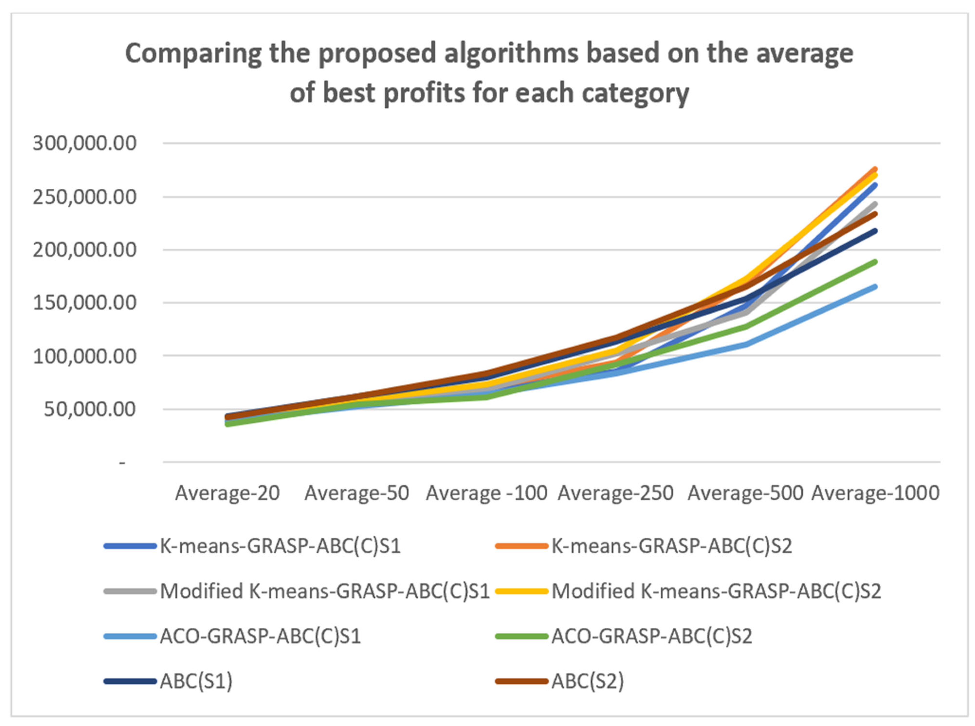
- Again, the methods used in the scout phase of the ABC seem to have an effect on the performance of the proposed algorithms. The first is the greedy randomised strategy, which selects a random customer pair, meaning the worst pair (either with low revenue or separated by a great distance) may be selected, resulting in poor solution quality. Moreover, in some cases, the neighbourhood operators cannot sufficiently enhance the quality of the solution because of time violations or load constraints. The second method uses the GRASP, which constructs solutions by randomly selecting from the Restricted Candidate List (RCL), which is half the size of the Candidate Solution Set (CSS). Thus, selecting unvisited customers is not a problem for small-sized instances because the number of customer pairs is small, which means the chance of selecting the best customer pair (i.e., that with the highest IR2 value) is high. In contrast, in medium- and large-sized instances, where the size of the RCL is large, the chance of selecting the best customer pair decreases, which affects the quality of the solutions.
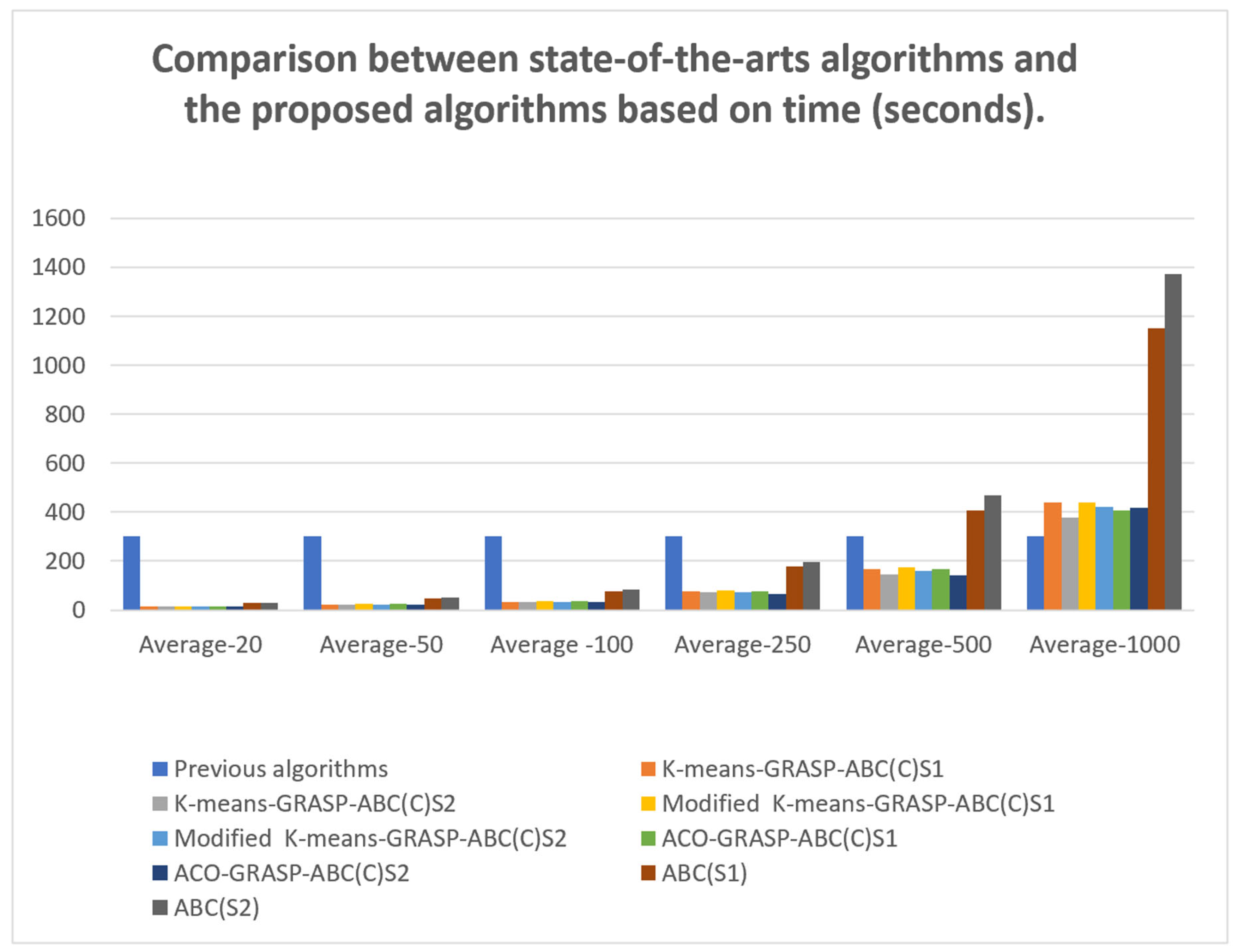
- The number of solutions in a population, the number of iterations, and the limit value play important roles in the algorithms’ performance. In our algorithms, we rely on small numbers of both solutions and iterations because a fast processing time is a critical demand for daily m-commerce apps. These decreased iteration numbers and population sizes, however, reduce the chances of achieving satisfactory solution quality.
- All previous algorithms were based on VNS, which has the ability to change the size of the neighbourhood search each time the solution quality is not enhanced. Thus, expanding the neighbourhood structure in a systematic way helps the VNS fully explore the neighbourhood and obtain good solutions. In contrast, the diversification feature in our approach is based either on the greedy feature (inserting the customer pair with the highest IR into the best position) or on a combination of greedy and randomised features (inserting a random customer pair into the best position or inserting a random customer pair from RCL into the best position). However, these strategies seem less successful at diversification than the VNS, which relies on an organised neighbourhood exploration mechanism.
6. Conclusions
Author Contributions
Funding
Data Availability Statement
Acknowledgments
Conflicts of Interest
References
- Curry, D. Food Delivery App Revenue and Usage Statistics. 2024. Available online: https://www.businessofapps.com/data/food-delivery-app-market/ (accessed on 24 January 2024).
- Khalid, H. Benefits of Food Delivery App for Restaurants and Customers. Available online: https://enatega.com/benefits-of-food-delivery-app/ (accessed on 1 February 2024).
- Team, D.J. Top Food Delivery Apps in Saudi Arabia 2023. Available online: https://www.digitalgravity.ae/blog/top-food-delivery-apps-in-saudi-arabia/ (accessed on 2 January 2024).
- Gansterer, M.; Küçüktepe, M.; Hartl, R.F. The multi-vehicle profitable pickup and delivery problem. OR Spectr. 2017, 39, 303–319. [Google Scholar] [CrossRef]
- Talbi, E.G. Metaheuristics: From Design to Implementation; John Wiley & Sons: Hoboken, NJ, USA, 2009; ISBN 978-0-470-27858-1. [Google Scholar]
- Alhujaylan, A.I.; Hosny, M.I. A GRASP-based solution construction approach for the multi-vehicle profitable pickup and delivery problem. Int. J. Adv. Comput. Sci. Appl. 2019, 10, 111–120. [Google Scholar] [CrossRef]
- Alhujaylan, A.I.; Hosny, M.I. Hybrid Clustering Algorithms with GRASP to Construct an Initial Solution for the MVPPDP. Comput. Mater. Contin. 2020, 62, 1025–1051. [Google Scholar] [CrossRef]
- Archetti, C.; Speranza, M.G.; Vigo, D. Vehicle routing problems with profits. In Vehicle Routing: Problems, Methods, and Applications, 2nd ed.; SIAM: Philadelphia, PA, USA, 2014; Chapter 10; pp. 273–297. ISBN 978-1-61197-358-7. [Google Scholar]
- Toth, P.; Vigo, D. Vehicle Routing: Problems, Methods, and Applications, 2nd ed.; Society for Industrial and Applied Mathematics: Philadelphia, PA, USA, 2015; ISBN 1611973589. [Google Scholar]
- Küçüktepe, M. A General Variable Neighbourhood Search Algorithm for the Multi-Vehicle Profitable Pickup and Delivery Problem. University of Vienna 2014. Available online: https://scholar.google.com/scholar?hl=en&as_sdt=0%2C5&q=A+General+Variable+Neighbourhood+Search+Algorithm+for+the+Multi-Vehicle+Profitable+Pickup+and+Delivery+Problem.+&btnG= (accessed on 22 June 2024).
- Haddad, M.N. An Efficient Heuristic for One-to-One Pickup and Delivery Problems. Ph.D. Thesis, IC/UFF, Niterói, Brazil, 2017. [Google Scholar]
- Bruni, M.E.; Toan, D.Q. The multi-vehicle profitable pick up and delivery routing problem with uncertain travel times. Transp. Res. Procedia 2021, 52, 509–516. [Google Scholar] [CrossRef]
- Karaboga, D. An Idea based on Honey Bee Swarm for Numerical Optimization. Technical Report-tr06, Erciyes University, Engineering Faculty, Computer Engineering Department. 2005. Available online: https://scholar.google.com/scholar?hl=en&as_sdt=0%2C5&q=An+idea+based+on+honey+bee+swarm+for+numerical+optimization&btnG= (accessed on 22 June 2024).
- Alazzawi, A.K.; Rais, H.M.; Basri, S.; Alsariera, Y.A. PhABC: A Hybrid Artificial Bee Colony Strategy for Pairwise test suite Generation with Constraints Support. In Proceedings of the 2019 IEEE Student Conference on Research and Development (SCOReD), Bandar Seri Iskandar, Malaysia, 15–17 October 2019; pp. 106–111, ISBN 9781728126135. [Google Scholar]
- Szeto, W.Y.; Wu, Y.; Ho, S.C. An artificial bee colony algorithm for the capacitated vehicle routing problem. Eur. J. Oper. Res. 2011, 215, 126–135. [Google Scholar] [CrossRef]
- Wu, B.; Shi, Z. A clustering algorithm based on swarm intelligence. In Proceedings of the 2001 International Conferences on Info-Tech and Info-Net. Proceedings (Cat. No.01EX479), Beijing, China, 29 October–1 November 2001; pp. 58–66, ISBN 0-7803-7010-4. [Google Scholar]
- Yao, B.; Hu, P.; Zhang, M.; Wang, S. Artificial bee colony algorithm with scanning strategy for the periodic vehicle routing problem. Simulation 2013, 89, 762–770. [Google Scholar] [CrossRef]
- Karaboga, D.; Akay, B. A survey: Algorithms simulating bee swarm intelligence. Artif. Intell. Rev. 2009, 31, 61–85. [Google Scholar] [CrossRef]
- Creutz, M. Microcanonical monte carlo simulation. Phys. Rev. Lett. 1983, 50, 1411. [Google Scholar] [CrossRef]
- Bansal, J.C.; Sharma, H.; Jadon, S.S. Artificial bee colony algorithm: A survey. Int. J. Adv. Intell. Paradig. 2013, 5, 123–159. [Google Scholar] [CrossRef]

| Dataset Instances | Number of Iterations | ||||
|---|---|---|---|---|---|
| 10 | 50 | 100 | 500 | 750 | |
| 13-100-F-S | 32,274.04 | 35,432.98 | 39,437.98 | 39,438.58 | 39,438.58 |
| 14-100-F-L | 63,311.86 | 63,311.86 | 63,311.86 | 63,455.13 | 63,455.13 |
| 15-100-P-S | 68,625.48 | 68,625.48 | 71,185.28 | 72,032.22 | 72,032.22 |
| 16-100-P-L | 115,792.8 | 115,792.8 | 124,608.2 | 131,404.9 | 131,404.9 |
| 17-100-R-S | 67,974.56 | 74,246.27 | 74,246.27 | 74,330.95 | 74,330.95 |
| 18-100-R-L | 112,986.9 | 112,986.9 | 116,775.2 | 119,991.9 | 119,991.9 |
| Dataset Instances | Population Size | |||
|---|---|---|---|---|
| 30 | 40 | 50 | 60 | |
| 13-100-F-S | 39,438.58 | 39,438.58 | 41,472.86 | 41,472.86 |
| 14-100-F-L | 63,455.13 | 66,453.66 | 66,453.66 | 66,453.66 |
| 15-100-P-S | 72,032.22 | 72,032.22 | 72,170.54 | 72,170.54 |
| 16-100-P-L | 131,404.9 | 131,404.9 | 131,404.9 | 131,404.9 |
| 17-100-R-S | 74,330.95 | 77,484.06 | 77,484.06 | 77,484.06 |
| 18-100-R-L | 119,991.9 | 120,249.7 | 126,504.3 | 126,504.3 |
| Dataset Instances | Limit | |
|---|---|---|
| 100 | 200 | |
| 13-100-F-S | 41,472.86 | 41,472.86 |
| 14-100-F-L | 66,453.66 | 66,453.66 |
| 15-100-P-S | 72,170.54 | 72,170.54 |
| 16-100-P-L | 131,404.9 | 131,404.9 |
| 17-100-R-S | 77,484.06 | 77,484.06 |
| 18-100-R-L | 126,504.3 | 126,504.3 |
| Dataset Instances | Demon Value | |||
|---|---|---|---|---|
| 1000 | 2500 | 5000 | 7500 | |
| 13-100-F-S | 41,472.86 | 41,596.33 | 41,954.86 | 41,954.86 |
| 14-100-F-L | 66,453.66 | 66,683.84 | 66,683.84 | 66,683.84 |
| 15-100-P-S | 72,170.54 | 72,449.56 | 72,449.56 | 72,449.56 |
| 16-100-P-L | 131,404.9 | 131,404.9 | 131,404.9 | 131,404.9 |
| 17-100-R-S | 77,484.06 | 77,484.06 | 77,484.06 | 77,484.06 |
| 18-100-R-L | 126,504.3 | 126,504.3 | 126,504.3 | 126,504.3 |
| Dataset | Previous Algorithms(5 min Runtime) | K-Means-GRASP-ABC(C)S1 | K-Means-GRASP-ABC(C)S2 | Modified K-Means-GRASP-ABC(C)S1 | Modified K-Means-GRASP-ABC(C)S2 | ACO-GRASP-ABC(C)S1 | ACO-GRASP-ABC(C)S2 | ABC(S1) | ABC(S2) |
| 1-20-F-S | 300 | 14.48 | 14.47 | 15.20 | 14.58 | 16.78 | 12.12 | 31.04 | 30.65 |
| 2-20-F-L | 300 | 12.13 | 12.42 | 13.82 | 13.17 | 13.51 | 11.45 | 30.20 | 30.56 |
| 3-20-P-S | 300 | 16.62 | 17.48 | 17.83 | 17.17 | 18.72 | 15.85 | 33.77 | 39.28 |
| 4-20-P-L | 300 | 12 | 12.01 | 12.61 | 12.24 | 15.63 | 12.98 | 24.43 | 28.45 |
| 5-20-R-S | 300 | 14.87 | 15.21 | 14.97 | 14.57 | 16.67 | 14.57 | 30.79 | 31.17 |
| 6-20-R-L | 300 | 11.32 | 12.38 | 13.47 | 13.71 | 13.63 | 12.25 | 22.62 | 21.56 |
| Average-20 | 300 | 13.57 | 14 | 14.65 | 14.24 | 15.82 | 13.20 | 28.81 | 30.28 |
| 7-50-F-S | 300 | 23.24 | 24.29 | 25.67 | 25.49 | 25.45 | 22.03 | 50.10 | 54.80 |
| 8-50-F-L | 300 | 19.79 | 21.24 | 21.53 | 21.45 | 22.18 | 20.65 | 43.81 | 46.63 |
| 9-50-P-S | 300 | 25.67 | 24.64 | 26.58 | 25.15 | 25.87 | 20.49 | 50.55 | 54.72 |
| 10-50-P-L | 300 | 21.63 | 22.64 | 24.41 | 22.96 | 23.34 | 20.90 | 44.77 | 48.77 |
| 11-50-R-S | 300 | 26.31 | 26.58 | 26.86 | 26.05 | 27.49 | 20.23 | 48.90 | 51.94 |
| 12-50-R-L | 300 | 22.73 | 20.93 | 23.37 | 21.87 | 22.77 | 20.91 | 45.94 | 48.34 |
| Average-50 | 300 | 23.23 | 23.39 | 24.74 | 23.83 | 24.52 | 20.87 | 47.34 | 50.86 |
| 13-100-F-S | 300 | 37.87 | 33.57 | 36.58 | 35.10 | 36.89 | 33.36 | 80.65 | 83.81 |
| 14-100-F-L | 300 | 31.42 | 33.67 | 34.59 | 34.38 | 35.55 | 33.14 | 73.90 | 81.74 |
| 15-100-P-S | 300 | 31.03 | 32.03 | 36.98 | 35.55 | 36.75 | 33.23 | 76.39 | 82.69 |
| 16-100-P-L | 300 | 33.54 | 34.33 | 36.50 | 34.57 | 36.20 | 32.41 | 74.19 | 82.93 |
| 17-100-R-S | 300 | 38 | 35.92 | 37 | 35.81 | 38.19 | 34.03 | 82.59 | 86.96 |
| 18-100-R-L | 300 | 36.19 | 35.37 | 34.38 | 33.34 | 37.49 | 33.63 | 77.02 | 81.01 |
| Average-100 | 300 | 34.68 | 34.15 | 36.01 | 34.79 | 36.85 | 33.30 | 77.46 | 83.19 |
| 19-250-F-S | 300 | 73.50 | 72.85 | 78.10 | 73.30 | 74.19 | 67.79 | 176.81 | 204.37 |
| 20-250-F-L | 300 | 79.65 | 73.28 | 80.50 | 76.28 | 77.66 | 65.10 | 181.10 | 195 |
| 21-250-P-S | 300 | 74.20 | 72.09 | 75.23 | 72.88 | 74.05 | 63.51 | 169.26 | 195.17 |
| 22-250-P-L | 300 | 73.82 | 72.718 | 79.53 | 74.40 | 77.86 | 65.44 | 179 | 193.60 |
| 23-250-R-S | 300 | 74.67 | 72.99 | 77.63 | 72.38 | 76.21 | 66.44 | 177.25 | 193.93 |
| 24-250-R-L | 300 | 79.55 | 73.21 | 84.04 | 73.84 | 79.62 | 69.46 | 178.99 | 194.47 |
| Average-250 | 300 | 75.90 | 72.86 | 79.17 | 73.85 | 76.60 | 66.29 | 177.07 | 196.09 |
| 25-500-F-S | 300 | 163.89 | 155.32 | 172.74 | 158.36 | 162.15 | 142.52 | 388.62 | 474.16 |
| 26-500-F-L | 300 | 167.03 | 155.73 | 177.18 | 160.25 | 170.25 | 148.98 | 415.25 | 466.38 |
| 27-500-P-S | 300 | 160.91 | 146.27 | 172.04 | 158.45 | 162.76 | 140.62 | 386.55 | 465.87 |
| 28-500-P-L | 300 | 168.60 | 144.23 | 180.26 | 158.74 | 169.89 | 141.34 | 435.34 | 464.62 |
| 29-500-R-S | 300 | 170.15 | 140.16 | 170.50 | 158.58 | 162.42 | 139.80 | 383.89 | 468.15 |
| 30-500-R-L | 300 | 169.78 | 141.24 | 174.22 | 161.07 | 169.30 | 143.36 | 428.65 | 464.89 |
| Average-500 | 300 | 166.73 | 147.16 | 174.49 | 159.24 | 166.13 | 142.77 | 406.38 | 467.35 |
| 31-1000-F-S | 300 | 432.51 | 354.73 | 448.29 | 408.67 | 426.32 | 397.22 | 1040.22 | 1406.22 |
| 32-1000-F-L | 300 | 439.85 | 360.11 | 447.72 | 423.01 | 461.18 | 430.54 | 1197.38 | 1438.43 |
| 33-1000-P-S | 300 | 434.34 | 364.52 | 432.93 | 418.51 | 391.01 | 416.76 | 1128.14 | 1398.49 |
| 34-1000-P-L | 300 | 448.06 | 378.57 | 440.70 | 435.69 | 389.93 | 430.39 | 1204.97 | 1416.64 |
| 35-1000-R-S | 300 | 451.79 | 404.20 | 425.83 | 421.47 | 381.24 | 411.31 | 1110.80 | 1296.40 |
| 36-1000-R-L | 300 | 420.15 | 410.26 | 446.23 | 418.03 | 393.29 | 420.10 | 1222.33 | 1286.07 |
| Average-1000 | 300 | 437.78 | 378.73 | 440.28 | 420.90 | 407.16 | 417.72 | 1150.64 | 1373.71 |
| Dataset | C1—Seq VNS [9] | C2—Seq VND [9] | C1—Self Adaptive VND [9] | C2—Self Adaptive VND [9] | IPPD [10] | K-Means-GRASP-ABC(C)S1 | K-Means-GRASP-ABC(C)S2 | Modified K-Means-GRASP-ABC(C)S1 | Modified K-Means-GRASP-ABC(C)S2 | ACO-GRASP-ABC(C)S1 | ACO-GRASP-ABC(C)S2 | ABC(S1) | ABC(S2) |
| 1-20-F-S | 30,315.5 | 30,315.5 | 30,315.5 | 30,315.5 | 30,315.5 | 30,267.75 | 30,427.58 | 27,007.58 | 27,007.58 | 25,490.76 | 25,490.76 | 30,395.92 | 30,294.77 |
| 2-20-F-L | 38,765.6 | 38,765.6 | 37,866.3 | 38,765.6 | 39,179.66 | 37,642.38 | 37,468.82 | 39,773.34 | 39,240.95 | 36,342.53 | 36,322.33 | 39,459.15 | 36,153.93 |
| 3-20-P-S | 51,473.4 | 52,128.4 | 52,565.1 | 52,565.1 | 52,566 | 51,481.8 | 43,340.71 | 51,481.8 | 43,009.55 | 42,917.34 | 34,107.64 | 52,684.98 | 52,565.1 |
| 4-20-P-L | 58,365.6 | 58,365.6 | 58,365.6 | 58,365.6 | 58,777 | 57,350.35 | 57,086.36 | 57,350.35 | 57,301.88 | 56,523.32 | 47,367.54 | 58,888.64 | 56,808.21 |
| 5-20-R-S | 36,469.5 | 36,469.5 | 36,469.5 | 36,469.5 | 36,469.5 | 34,090.58 | 34,090.58 | 30,237.02 | 29,843.58 | 31,741.08 | 31,741.08 | 36,469.52 | 36,469.52 |
| 6-20-R-L | 43,368.6 | 43,368.6 | 43,368.6 | 43,368.6 | 43,781.81 | 42,215.53 | 42,086.44 | 44,401.45 | 43,736.53 | 40,769.67 | 40,450.55 | 44,244.27 | 42,143.26 |
| Average-20 | 43,126.37 | 43,235.53 | 43,158.43 | 43,308.32 | 43,514.91 | 42,174.73 | 40,750.08 | 41,708.59 | 40,023.35 | 38,964.12 | 35,913.32 | 43,690.41 | 42,405.8 |
| Standard Deviation | 10,289.94 | 10,399.10 | 10,559.14 | 10,475.04 | 10,560.13 | 10,436.42 | 9349.23 | 11,822.81 | 10,907.82 | 10,656.36 | 7500.01 | 10,573.40 | 10,312.25 |
| 7-50-F-S | 22,306 | 22,306 | 22,306 | 22,306 | 22,307.15 | 18,662.83 | 21,603.83 | 18,662.83 | 21,603.83 | 21,281.88 | 25,123.15 | 24,975.25 | 24,998.45 |
| 8-50-F-L | 58,050.8 | 58,050.8 | 57,303.4 | 57,996.7 | 58,050.8 | 50,772.64 | 50,873.68 | 50,881.55 | 50,773.54 | 46,699.31 | 47,534.79 | 53,555.25 | 53,268.82 |
| 9-50-P-S | 57,651.7 | 57,651.7 | 57,651.7 | 57,651.7 | 57,651.7 | 58,996.17 | 53,258.83 | 58,996.17 | 53,064.14 | 55,643.25 | 55,643.25 | 57,651.71 | 57,651.71 |
| 10-50-P-L | 132,648 | 132,648,0 | 128,353 | 128,334.8 | 129,640.3 | 109,726.8 | 117,770.8 | 116,372 | 116,149.7 | 97,740.02 | 106,491.9 | 124,819.3 | 128,477.1 |
| 11-50-R-S | 33,340.4 | 33,340.4 | 33,340.4 | 33,340.4 | 33,340.4 | 28,865.48 | 28,907.33 | 28,865.48 | 28,907.33 | 31,251.34 | 29,969.16 | 33,054.57 | 33,098.58 |
| 12-50-R-L | 79,350.3 | 79,350.3 | 77,655.5 | 79,350.3 | 77,832.56 | 76,422.62 | 76,503.28 | 76,309.46 | 76,408.91 | 64,359.55 | 64,519.79 | 76,582.15 | 75,732.86 |
| Average-50 | 63,891.2 | 50,139.84 | 62,768.33 | 63,163.32 | 63,137.16 | 57,241.09 | 58,152.95 | 58,347.92 | 57,817.91 | 52,829.22 | 54,880.35 | 61,773.03 | 62,204.58 |
| Standard Deviation | 39,248.45 | 22,523.36 | 37,635.69 | 37,749.54 | 38,077.61 | 33,048.63 | 35,097.31 | 35,184.37 | 34,547.72 | 27,041.68 | 29,384.58 | 35,937.41 | 37,167.44 |
| 13-100-F-S | 41,464.84 | 41,955.2 | 41,523.5 | 42,174 | 41,896.86 | 35,386.24 | 36,055.01 | 35,303.67 | 36,625.9 | 33,147.92 | 33,187.57 | 40,596.77 | 40,543.56 |
| 14-100-F-L | 81,271.2 | 81,971 | 80,080.4 | 80,500.2 | 79,479.88 | 58,704.7 | 60,780.74 | 57,607.07 | 60,035.43 | 51,106.58 | 47,074.98 | 64,937.47 | 67,237.63 |
| 15-100-P-S | 70,387.4 | 70,398.5 | 71,113.8 | 71,082.8 | 69,436.25 | 54,197 | 57,206.6 | 49,566.36 | 59,481.84 | 60,614.78 | 45,995.09 | 68,874.02 | 71,290.33 |
| 16-100-P-L | 124,288 | 123,931 | 122,691.8 | 122,183.2 | 125,057 | 98,140.3 | 104,031.6 | 100,122.4 | 110,099 | 92,681.38 | 96,365.75 | 112,690.5 | 124,487.1 |
| 17-100-R-S | 76,885.4 | 78,418.8 | 76,954.4 | 79,651.2 | 77,012.75 | 61,579.81 | 61,579.81 | 61,960.78 | 61,698.84 | 52,689.7 | 52,163.72 | 77,334.8 | 75,925.47 |
| 18-100-R-L | 131,052.6 | 130,670.4 | 130,403.4 | 130,366.6 | 131,058.6 | 98,522.81 | 100,291.3 | 104,771.9 | 109,450.2 | 92,423.54 | 93,867.6 | 115,108.7 | 122,320.4 |
| Average-100 | 87,558.24 | 87,890.82 | 87,127.88 | 87,659.67 | 87,323.56 | 67,755.14 | 69,990.84 | 68,222.03 | 72,898.54 | 63,777.32 | 61,442.45 | 79,923.7 | 83,634.09 |
| Standard Deviation | 34,099 | 33,674.36 | 33,546.8 | 33,090.45 | 34,316.01 | 25,383.15 | 26,636.59 | 28,060.86 | 30,021.67 | 24,032.04 | 26,834.7 | 29,022.89 | 33,175.38 |
| 19-250-F-S | 73,259.94 | 72,445.3 | 72,703 | 72,287.9 | 70,799.19 | 36,045.94 | 32,341.35 | 43,729.29 | 38,692.81 | 34,038.31 | 33,942.57 | 48,988.62 | 46,216.19 |
| 20-250-F-L | 132,996 | 132,438 | 132,394.4 | 133,404 | 129,485.3 | 54,144.64 | 63,245.12 | 70,325.74 | 81,370.79 | 51,239.48 | 57,273.9 | 71,397.91 | 81,288.1 |
| 21-250-P-S | 111,334.4 | 111,817.8 | 109,449.4 | 109,355.8 | 110,440.3 | 62,245.05 | 71,066.44 | 74,931.5 | 83,992.55 | 72,198.2 | 69,410.97 | 86,624.32 | 93,568.56 |
| 22-250-P-L | 197,899.8 | 197,214.2 | 194,131.2 | 194,549 | 194,338.6 | 112,454.5 | 131,917.5 | 133,567.4 | 155,750.3 | 95,906.32 | 127,789.5 | 146,104 | 160,301.3 |
| 23-250-R-S | 162,410.8 | 162,448.2 | 158,164.4 | 159,129.6 | 158,414.6 | 99,900 | 90,042.33 | 109,717.8 | 93,812.47 | 102,500.1 | 99,734.68 | 125,201.2 | 120,776 |
| 24-250-R-L | 269,072.8 | 268,713.8 | 266,559 | 267,291.4 | 266,204.2 | 148,156.7 | 176,579.9 | 180,807.7 | 177,336 | 146,270.4 | 164,012.2 | 204,037.4 | 203,859.8 |
| Average-250 | 157,829 | 157,512.9 | 155,566.9 | 156,003 | 154,947 | 85,491.14 | 94,198.78 | 102,179.9 | 105,159.2 | 83,692.14 | 92,027.3 | 113,725.6 | 117,668.3 |
| Standard Deviation | 69,184.1 | 69,165.71 | 68,327.76 | 68,666.69 | 68,777.74 | 42,022.43 | 52,050.37 | 49,795.51 | 51,632.15 | 40,174 | 48,193.98 | 56,662.62 | 57,036.7 |
| 25-500-F-S | 158,425.4 | 159,146.2 | 157,399.8 | 159,526.6 | 155,683.9 | 59,737.27 | 71,001.31 | 51,581.38 | 73,939.03 | 54,762.97 | 51,117.39 | 75,731.5 | 79,862.1 |
| 26-500-F-L | 243,210 | 244,591.6 | 245,600.8 | 245,183.6 | 242,173.1 | 101,753.4 | 120,779.3 | 106,505.3 | 129,200.4 | 62,041.19 | 88,256.7 | 112,172 | 121,824.9 |
| 27-500-P-S | 201,195.4 | 202,102.2 | 197,227.6 | 198,740 | 203,932.9 | 105,678.8 | 146,631.6 | 107,797.6 | 143,918.5 | 102,996.9 | 105,667.8 | 130,361.2 | 143,638.1 |
| 28-500-P-L | 319,239.2 | 321,181.6 | 315,854.6 | 317,610.8 | 329,642.8 | 229,525.6 | 241,331.4 | 225,812.4 | 243,361.8 | 152,573.5 | 191,169.5 | 201,973.8 | 222,042.1 |
| 29-500-R-S | 271,154.4 | 272,715.2 | 271,264.2 | 273,095 | 260,505.8 | 126,298.6 | 156,901.1 | 108,998.5 | 162,660.4 | 127,089.1 | 123,505.3 | 166,111.6 | 166,226.9 |
| 30-500-R-L | 402,557.2 | 406,689.6 | 399,990.8 | 404,517 | 408,819.4 | 259,683.6 | 272,509 | 241,454 | 282,087 | 167,819.5 | 205,885.1 | 239,675.7 | 255,261.1 |
| Average-500 | 265,963.6 | 267,737.7 | 264,556.3 | 266,445.5 | 266,793 | 147,112.9 | 168,192.3 | 140,358.2 | 172,527.9 | 111,213.8 | 127,600.3 | 154,337.6 | 164,809.2 |
| Standard Deviation | 69,184.1 | 69,165.71 | 68,327.76 | 68,666.69 | 68,777.74 | 42,022.43 | 52,050.37 | 49,795.51 | 51,632.15 | 40,174 | 48,193.98 | 56,662.62 | 57,036.7 |
| 31-1000-F-S | 150,920.4 | 151,943.2 | 151,990 | 153,820.6 | 152,358.7 | 33,184.03 | 48,758.35 | 39,530.22 | 48,457.57 | 23,266.5 | 20,723.05 | 33,125.19 | 41,340.89 |
| 32-1000-F-L | 218,211 | 218,213 | 223,999.8 | 222,072.8 | 222,089.1 | 92,970.35 | 93,386.23 | 92,142.15 | 95,500.88 | 24,110.85 | 44,359.35 | 57,137.24 | 68,705.69 |
| 33-1000-P-S | 439,681.8 | 441,120.2 | 433,353.8 | 429,853 | 457,759.4 | 272,126.9 | 288,095.1 | 236,797.1 | 280,912.6 | 178,654.3 | 201,178.4 | 240,944.9 | 263,540.2 |
| 34-1000-P-L | 678,396.2 | 651,754.6 | 677,511.6 | 669,212.8 | 681,370.5 | 498,835.3 | 519,115.5 | 492,753.1 | 507,105.4 | 346,244.9 | 366,004.4 | 397,930 | 426,372.5 |
| 35-1000-R-S | 455,054.6 | 461,394 | 459,167.4 | 462,999.2 | 461,919.6 | 207,134 | 255,835.4 | 192,030.8 | 242,210.5 | 124,538.1 | 176,577.1 | 212,979.1 | 228,716 |
| 36-1000-R-L | 668,655 | 662,605.4 | 668,615.4 | 667,184.8 | 676,159.7 | 464,549.3 | 450,834.3 | 407,703.7 | 448,210.5 | 297,212.8 | 322,568.7 | 364,643.1 | 372,491.4 |
| Average-1000 | 435,153.2 | 431,171.7 | 435,773 | 434,190.5 | 441,942.8 | 261,466.7 | 276,004.1 | 243,492.9 | 270,399.6 | 165,671.2 | 188,568.5 | 217,793.2 | 233,527.8 |
| Standard Deviation | 219,981.4 | 212,861.8 | 218,443.1 | 216,320 | 221,371.6 | 190,345 | 187,196 | 176,803.2 | 183,520.7 | 135,712.2 | 140,506.7 | 151,318.2 | 155,901.2 |
| Dataset | Best Known Profit | C1—Seq VNS [4] | C2—Seq VND [4] | C1—Self Adaptive VND [4] | C2—Self Adaptive VND [4] | IPPD [10] | K-Means-GRASP-ABC(C)S1 | ||||||||||||
| Best Profit | Gap | Best Profit | Gap | Best Profit | Gap | Best Profit | Gap | Best Profit | Gap | Best Profit | Gap | ||||||||
| 1-20-F-S | 30,315.5 | 30,315.5 | 0 | 30,315.5 | 0 | 30,315.5 | 0 | 30,315.5 | 0 | 30,315.5 | 0 | 30,267.75 | −0.15 | ||||||
| 2-20-F-L | 39,340.3 | 38,765.6 | −1.5 | 38,765.6 | −1.5 | 38,765.6 | −1.5 | 38,765.6 | −1.5 | 39,179.66 | −0.41 | 37,750.35 | −4 | ||||||
| 3-20-P-S | 52,855.2 | 51,473.4 | 2.7 | 52,561.1 | −0.6 | 52,565.1 | −0.6 | 52,565.1 | −0.6 | 52,566 | −0.55 | 51,515.53 | −2.5 | ||||||
| 4-20-P-L | 58,365.6 | 58,365.6 | 0 | 58,365.6 | 0 | 58,365.6 | 0 | 58,365.6 | 0 | 58,777 | 0.7 | 57,350.35 | −1.7 | ||||||
| 5-20-R-S | 36,469.5 | 36,469.5 | 0 | 36,469.5 | 0 | 36,469.5 | 0 | 36,469.5 | 0 | 36,469.5 | 0 | 34,090.58 | −6.5 | ||||||
| 6-20-R-L | 43,764.3 | 43,368.6 | −0.9 | 43,368.6 | −0.9 | 43,368.6 | −0.9 | 43,368.6 | −0.9 | 43,781.81 | 0.04 | 42,353.35 | −3.2 | ||||||
| Average-20 | 43,518.4 | 43,126.37 | −0.85 | 43,307.65 | −0.50 | 43,308.32 | −0.50 | 43,308.32 | −0.50 | 43,514.91 | −0.04 | 42,221.32 | −2.9 | ||||||
| 7-50-F-S | 22,441 | 22,306 | −0.6 | 22,306 | −0.6 | 22,306 | −0.6 | 22,306 | −0.6 | 22,307.15 | −0.6 | 18,662.83 | −16.8 | ||||||
| 8-50-F-L | 58,050.8 | 58,050.8 | 0 | 58,050.8 | 0 | 58,050.8 | 0 | 58,050.8 | 0 | 58,050.8 | 0 | 51,040.14 | −12 | ||||||
| 9-50-P-S | 57,651.7 | 57,651.7 | 0 | 57,651.7 | 0 | 57,651.7 | 0 | 57,651.7 | 0 | 57,651.7 | 0 | 58,996.17 | 2.3 | ||||||
| 10-50-P-L | 132,648 | 132,648 | 0 | 132,648 | 0 | 132,648 | 0 | 132,648 | 0 | 132,648 | 0 | 114,962.9 | −13.3 | ||||||
| 11-50-R-S | 33,340.4 | 33,340.4 | 0 | 33,340.4 | 0 | 33,340.4 | 0 | 33,340.4 | 0 | 33,340.4 | 0 | 28,907.33 | −13.2 | ||||||
| 12-50-R-L | 79,350.3 | 79,350.3 | 0 | 79,350.3 | 0 | 79,350.3 | 0 | 79,350.3 | 0 | 77,832.56 | −1.95 | 76,479.84 | −3.6 | ||||||
| Average-50 | 63,913.7 | 63,891.20 | −0.1 | 63,891.20 | −0.10 | 63,891.20 | −0.10 | 63,891.20 | −0.10 | 63,638.44 | −0.43 | 58,174.87 | −8.9 | ||||||
| 13-100-F-S | 44,402.3 | 42,174.4 | −5.3 | 42,174.4 | −5.3 | 42,174.4 | −5.3 | 42,215.5 | −5.2 | 41,956.25 | −5.83 | 36,322.94 | −18.1 | ||||||
| 14-100-F-L | 81,999.4 | 81,999.4 | 0 | 81,999.4 | 0 | 81,621 | −0.5 | 80,848.1 | −0.2 | 88,891.4 | 0 | 60,767.96 | −25.8 | ||||||
| 15-100-P-S | 71,512.4 | 70,836 | −1 | 71,326.4 | −0.3 | 71,399.2 | −0.2 | 71,399.2 | −0.2 | 71,234.58 | −0.39 | 54,428.34 | −23.8 | ||||||
| 16-100-P-L | 125,032 | 124,770 | −0.2 | 124,770 | −0.2 | 123,766 | −1 | 124,910 | −0.1 | 125,786.7 | −0.6 | 99,860.9 | −20.1 | ||||||
| 17-100-R-S | 80,878.8 | 80,878.8 | 0 | 78,818 | −2.6 | 80,878.8 | 0 | 80,878.8 | 0 | 80,878.8 | 0 | 61,647.98 | −23.7 | ||||||
| 18-100-R-L | 131,845 | 131,473 | −0.3 | 131,845 | 0 | 131,339 | −0.4 | 131,339 | −0.4 | 131,845 | 0 | 102,403.8 | −22.3 | ||||||
| Average-100 | 89,278.32 | 97,991.44 | −1.13 | 88,488.87 | −1.40 | 88,529.73 | −1.23 | 88,598.43 | −1.02 | 90,098.79 | −1.14 | 69,238.65 | −22.4 | ||||||
| 19-250-F-S | 75,309.1 | 73,610.9 | −2.3 | 73,575.7 | −2.4 | 73,835.5 | 2 | 73,544,7 | −2.4 | 72,038.6 | −4.54 | 39,672.94 | −47.3 | ||||||
| 20-250-F-L | 136,594 | 134,889 | −1.3 | 134,186 | −1.8 | 132,870 | −2.8 | 135,622 | −0.7 | 131,012.9 | −4.26 | 54,144.64 | −60.3 | ||||||
| 21-250-P-S | 113,886 | 112,427 | −1.3 | 112,480 | −1.3 | 112,428 | −1.3 | 110,062 | −3.5 | 112,747.3 | −1.01 | 69,574.44 | −38.9 | ||||||
| 22-250-P-L | 200,402 | 200,402 | 0 | 198,611 | −0.9 | 195,135 | −2.7 | 196,524 | −2 | 198,241.2 | −1.09 | 112,454.5 | −43.8 | ||||||
| 23-250-R-S | 164,070 | 162,960 | −0.7 | 164,070 | 0 | 162,115 | −1.2 | 162,115 | −1.2 | 161,804.7 | −1.4 | 103,456 | −36.9 | ||||||
| 24-250-R-L | 274,563 | 271,185 | −1.2 | 271,193 | −1.2 | 272,957 | −0.6 | 269,790 | −1.8 | 269,734.7 | −1.79 | 148,156.7 | −46 | ||||||
| Average-250 | 160,804 | 159,245.65 | −1.13 | 159,019.28 | −1.27 | 158,223.42 | −1.10 | 174,822.60 | −1.93 | 157,596.57 | −2.35 | 87,909.87 | −45.3 | ||||||
| 25-500-F-S | 167,080 | 161,063 | −3.7 | 161,040 | −3.8 | 159,064 | −5 | 161,375 | −3.5 | 160,592.1 | −4.04 | 59,737.27 | −64.2 | ||||||
| 26-500-F-L | 259,319 | 249,171 | −4.1 | 249,661 | −3.9 | 247,986 | −4.6 | 249,312 | −4 | 249,105.7 | −4.1 | 107,852.1 | −58.4 | ||||||
| 27-500-P-S | 206,788 | 203,832 | −1.5 | 205,480 | −0.6 | 200,764 | −3 | 201,590 | −2.6 | 208,287.7 | 0.72 | 105,678.8 | −48.8 | ||||||
| 28-500-P-L | 331,291 | 321,471 | −3.1 | 325,522 | −1.8 | 320,872 | −3.2 | 321,155 | −3.2 | 337,358.9 | 1.82 | 229,525.6 | −30.7 | ||||||
| 29-500-R-S | 281,711 | 279,105 | −0.9 | 278,233 | −1.3 | 274,419 | −2.7 | 276,392 | −1.9 | 265,040 | −6.29 | 126,298.6 | −55.1 | ||||||
| 30-500-R-L | 417,282 | 407,689 | −2.4 | 409,755 | −1.8 | 407,849 | −2.3 | 409,262 | −2 | 411,967.6 | −1.29 | 259,683.6 | −37.7 | ||||||
| Average-500 | 277,245.2 | 270,388.50 | −2.61 | 271,615.17 | −2.20 | 268,492.33 | −3.47 | 269,847.67 | −2.87 | 272,058.67 | −2.20 | 165,807.7 | −40.1 | ||||||
| 31-1000-F-S | 173,826 | 154,196 | −12.7 | 151,943.2 | −12.2 | 154,357 | −12.6 | 156,106 | −11.4 | 152,358.7 | −11.8 | 33,184.03 | −80.9 | ||||||
| 32-1000-F-L | 247,385 | 221,958 | −11.5 | 221,322 | −11.8 | 224,999 | −9.9 | 226,913 | −9 | 222,089.1 | −10.1 | 92,970.35 | −62.4 | ||||||
| 33-1000-P-S | 464,580 | 450,349 | −3.2 | 450,337 | −3.2 | 442,311 | −5 | 442,218 | −5.1 | 457,759.4 | 1.47 | 272,126.9 | −41.4 | ||||||
| 34-1000-P-L | 712,918 | 693,407 | −2.8 | 672,910 | −5.9 | 684,121 | −4.2 | 683,211 | −4.3 | 681,370.5 | −3.26 | 498,835.3 | −30 | ||||||
| 35-1000-R-S | 492,083 | 463,625 | −6.1 | 472,626 | −4.1 | 465,022 | −5.8 | 469,162 | −4.9 | 461,919.6 | −4.90 | 207,134 | −57.9 | ||||||
| 36-1000-R-L | 705,167 | 673,951 | −4.6 | 669,926 | −5.3 | 676,720 | −4.4 | 684,217 | −3.1 | 676,159.7 | −2.90 | 464,549.3 | −34.1 | ||||||
| Average-1000 | 465,993.2 | 405,958 | −6.8 | 439,844.03 | −7.08 | 441,255 | −6.98 | 443,638 | −6.3 | 441,942.83 | −5.2 | 261,466.65 | −43.8 | ||||||
| Dataset | K-Means-GRASP-ABC(C)S2 | Modified K-Means-GRASP-ABC(C)S1 | Modified K-Means-GRASP-ABC(C)S2 | ACO-GRASP-ABC(C)S1 | ACO-GRASP-ABC(C)S2 | ABC(S1) | ABC(S2) | ||||||||||||
| Best Profit | Gap | Best Profit | Gap | Best Profit | Gap | Best Profit | Gap | Best Profit | Gap | Best Profit | Gap | Best Profit | Gap | ||||||
| 1-20-F-S | 30,427.58 | 0.3 | 27,007.58 | −10.9 | 27,007.58 | −10.9 | 25,490.76 | −15.9 | 25,490.76 | −15.9 | 30,554.62 | 0.78 | 30,315.52 | 0 | |||||
| 2-20-F-L | 37,556.07 | −4.5 | 40,104.23 | 1.9 | 39,240.95 | −0.2 | 36,423.3 | −7.4 | 36,322.33 | −7.6 | 40,104.23 | 1.9 | 36,234.48 | −7.8 | |||||
| 3-20-P-S | 44,334.2 | −16.1 | 51,515.53 | −2.5 | 44,334.2 | −16.1 | 42,944.78 | −18.7 | 34,107.64 | −35.4 | 53,164.53 | 0.58 | 52,565.1 | −0.5 | |||||
| 4-20-P-L | 57,350.35 | −1.7 | 57,350.35 | −1.7 | 57,350.35 | −1.7 | 56,603.63 | −3 | 47,402.91 | −18.7 | 59,140.98 | 1.32 | 57,286.89 | −1.8 | |||||
| 5-20-R-S | 34,090.58 | −6.5 | 30,827.18 | −15.4 | 29,843.58 | −18.1 | 31,741.08 | −12.9 | 31,741.08 | −12.9 | 36,469.52 | 0 | 36,469.52 | 0 | |||||
| 6-20-R-L | 42,169.13 | −3.6 | 44,764.07 | 2.2 | 43,780.72 | 0.04 | 41,071.62 | −6.1 | 40,600.21 | −7.2 | 44,707.23 | 2.1 | 42,873.71 | −2 | |||||
| Average-20 | 40,987.99 | −5.8 | 41,928.16 | −3.6 | 40,259.56 | −7.4 | 39,045.86 | −10.2 | 35,944.16 | −17.4 | 44,023.52 | 1.16 | 42,624.2 | −2 | |||||
| 7-50-F-S | 21,603.83 | −3.7 | 21,603.83 | −3.7 | 21,603.83 | −3.7 | 21,281.88 | −5.1 | 25,123.15 | 11.9 | 24,975.25 | 11.2 | 24,998.45 | 11.3 | |||||
| 8-50-F-L | 51,001.04 | −12.1 | 51,001.04 | −12.1 | 50,896.3 | −12.3 | 49,128.45 | −15.3 | 50,061.24 | −13.7 | 53,710.99 | −7.4 | 54,288.08 | −6.4 | |||||
| 9-50-P-S | 54,165.39 | −6 | 54,165.39 | −6 | 53,064.14 | −7.9 | 55,643.25 | −3.4 | 55,643.25 | −3.4 | 57,651.71 | 0 | 57,651.71 | 0 | |||||
| 10-50-P-L | 119,099.6 | −10.2 | 119,099.6 | −10.2 | 116,868.6 | −11.8 | 100,393.3 | −24.3 | 106,544.8 | −19.6 | 126,360 | −4.7 | 133,743.2 | 0.82 | |||||
| 11-50-R-S | 28,907.33 | −13.2 | 28,907.33 | −13.2 | 28,907.33 | −13.2 | 31,251.34 | −6.2 | 29,969.16 | −10.1 | 33,058.21 | −0.8 | 33,159.12 | −0.5 | |||||
| 12-50-R-L | 76,697.65 | −3.3 | 76,697.65 | −3.3 | 76,604.84 | −3.4 | 65,792.21 | −17 | 65,752.8 | −17.1 | 77,467.34 | −2.3 | 76,517.36 | −3.5 | |||||
| Average-50 | 58,579.14 | −8.3 | 58,579.14 | −8.3 | 57,990.84 | −9.2 | 53,915.07 | −15.6 | 55,515.73 | −13.1 | 62,203.92 | −2.6 | 63,392.99 | −0.8 | |||||
| 13-100-F-S | 36,188.32 | −18.4 | 35,937.96 | −19 | 38,323.6 | −13.6 | 33,565.46 | −24.4 | 33,566.06 | −24.4 | 41,812.08 | −5.8 | 41,636.8 | −6.2 | |||||
| 14-100-F-L | 63,488.24 | −22.5 | 60,851.27 | −25.7 | 61,351.99 | −25.1 | 52,328.66 | −36.1 | 49,789.52 | −39.2 | 66,375.92 | −19 | 72,595.41 | −11.4 | |||||
| 15-100-P-S | 60,815.37 | −14.9 | 54,190.18 | −24.2 | 60,554.49 | −15.3 | 60,614.78 | −15.2 | 47,498.28 | −33.5 | 69,275.79 | −3.1 | 71,400.63 | −0.1 | |||||
| 16-100-P-L | 104,786.4 | −16.1 | 102,121.7 | −18.3 | 111,728.2 | −10.6 | 95,836.25 | −23.3 | 101,142.5 | −19.1 | 115,579.2 | −7.5 | 128,473.2 | 2.7 | |||||
| 17-100-R-S | 61,647.98 | −23.7 | 61,962.79 | −23.3 | 61,962.79 | −23.3 | 52,689.7 | −34.8 | 52,689.7 | −34.8 | 77,484.06 | −4.1 | 77,484.06 | −4.1 | |||||
| 18-100-R-L | 101,013.6 | −23.3 | 105,175.3 | −20.2 | 110,683.8 | −16 | 95,363.69 | −27.6 | 97,568.94 | −25.9 | 119,554.3 | −9.3 | 126,871.5 | −3.7 | |||||
| Average-100 | 71,323.32 | −20.1 | 70,039.87 | −21.5 | 74,100.81 | −17 | 65,066.42 | −27.1 | 63,709.17 | −28.6 | 81,680.23 | −8.5 | 86,410.27 | −3.2 | |||||
| 19-250-F-S | 35,443.33 | −52.9 | 48,079.56 | −36.1 | 39,848.03 | −47 | 36,309.86 | −51.7 | 36,612.19 | −51.3 | 36,309.86 | −51.7 | 36,612.19 | −51.3 | |||||
| 20-250-F-L | 67,014.68 | −50.9 | 70,325.74 | −48.5 | 87,575.52 | −35.8 | 51,239.48 | −62.4 | 62,831.21 | −54 | 51,239.48 | −62.4 | 62,831.21 | −54 | |||||
| 21-250-P-S | 77,941.82 | −31.5 | 81,510.78 | −28.4 | 92,124.73 | −19.1 | 73,654.78 | −35.3 | 73,143.68 | −35.7 | 73,654.78 | −35.3 | 73,143.68 | −35.7 | |||||
| 22-250-P-L | 135,164.3 | −32.5 | 133,567.4 | −33.3 | 161,377.2 | −19.4 | 95,906.32 | −52.1 | 131,668.8 | −34.2 | 95,906.32 | −52.1 | 131,668.8 | −34.2 | |||||
| 23-250-R-S | 97,231.36 | −40.7 | 113,547.4 | −30.7 | 95,471.16 | −41.8 | 107,628.9 | −34.4 | 101,863.1 | −37.9 | 107,628.9 | −34.4 | 101,863.1 | −37.9 | |||||
| 24-250-R-L | 187,891.9 | −31.5 | 180,807.7 | −34.1 | 180,803 | −34.1 | 146,270.4 | −46.7 | 166,523.5 | −39.3 | 146,270.4 | −46.7 | 166,523.5 | −39.3 | |||||
| Average-250 | 100,114.6 | −37.7 | 104,639.8 | −34.9 | 109,533.3 | −31.8 | 85,168.2 | −47 | 95,440.4 | −40.6 | 85,168.2 | −47 | 95,440.4 | −40.6 | |||||
| 25-500-F-S | 74,692.46 | −55.2 | 51,581.38 | −69.1 | 76,481.48 | −54.2 | 61,718.84 | −63 | 54,247.37 | −67.5 | 78,432.78 | −53 | 86,250.21 | −48.3 | |||||
| 26-500-F-L | 124,478.4 | −51.9 | 106,505.3 | −58.9 | 131,572.4 | −49.2 | 72,388.37 | −72 | 93,308.66 | −64 | 112,172 | −56.7 | 126,203.2 | −51.3 | |||||
| 27-500-P-S | 152,566.6 | −26.2 | 107,797.6 | −47.8 | 150,645.3 | −27.1 | 109,238 | −47.1 | 112,111.9 | −45.7 | 136,168.2 | −34.1 | 148,384.5 | −28.2 | |||||
| 28-500-P-L | 249,759.7 | −24.6 | 225,812.4 | −31.8 | 247,180.6 | −25.3 | 152,573.5 | −53.9 | 196,969.2 | −40.5 | 201,973.8 | −39 | 225,040.5 | −32 | |||||
| 29-500-R-S | 172,397.2 | −38.8 | 108,998.5 | −61.3 | 175,267.1 | −37.7 | 141,743.7 | −49.6 | 128,570.6 | −54.3 | 178,693.9 | −36.5 | 173,003.3 | −38.5 | |||||
| 30-500-R-L | 275,488.2 | −33.9 | 241,454 | −42.1 | 294,424.7 | −29.4 | 167,819.5 | −59.7 | 214,081.3 | −48.6 | 239,675.7 | −42.5 | 261,517.2 | −37.3 | |||||
| Average-500 | 174,897.1 | −36.9 | 140,358.2 | −49.3 | 179,261.9 | −35.3 | 117,580.3 | −57.5 | 133,214.8 | −51.9 | 157,852.7 | −43 | 170,066.5 | −38.6 | |||||
| 31-1000-F-S | 51,188.29 | −70.5 | 39,530.22 | −77.2 | 51,585.38 | −70.3 | 23,266.5 | −86.6 | 25,563.9 | −85.2 | 33,125.19 | −80.9 | 42,197.08 | −75.7 | |||||
| 32-1000-F-L | 97,093.51 | −60.7 | 92,142.15 | −62.7 | 97,772.35 | −60.4 | 24,110.85 | −90.2 | 47,620.03 | −80.7 | 57,137.24 | −76.9 | 73,126.9 | −70.4 | |||||
| 33-1000-P-S | 293,900.2 | −36.7 | 236,797.1 | −49 | 287,774.9 | −38 | 178,654.3 | −61.5 | 209,372.1 | −54.9 | 240,944.9 | −48.1 | 267,814.2 | −42.3 | |||||
| 34-1000-P-L | 536,199.8 | −24.7 | 492,753.1 | −30.8 | 534,689.9 | −24.9 | 346,244.9 | −51.4 | 381,116.4 | −46.5 | 397,930 | −44.1 | 430,894.4 | −39.5 | |||||
| 35-1000-R-S | 264,295.2 | −46.2 | 192,030.8 | −60.9 | 249,078.6 | −49.3 | 124,538.1 | −74.6 | 181,237 | −63.1 | 212,979.1 | −56.7 | 232,298.7 | −52.7 | |||||
| 36-1000-R-L | 458,126.7 | −35 | 407,703.7 | −42.1 | 463,915.7 | −34.2 | 297,212.8 | −57.8 | 335,935.6 | −52.3 | 364,643.1 | −48.2 | 380,268.9 | −46 | |||||
| Average-1000 | 276,004.15 | −40.7 | 243,492.8 | −47.7 | 280,802.8 | −39.7 | 165,671.2 | −64.4 | 196,807.5 | −57.7 | 217,793.3 | −53.2 | 237,766.7 | −48.9 | |||||
Disclaimer/Publisher’s Note: The statements, opinions and data contained in all publications are solely those of the individual author(s) and contributor(s) and not of MDPI and/or the editor(s). MDPI and/or the editor(s) disclaim responsibility for any injury to people or property resulting from any ideas, methods, instructions or products referred to in the content. |
© 2024 by the authors. Licensee MDPI, Basel, Switzerland. This article is an open access article distributed under the terms and conditions of the Creative Commons Attribution (CC BY) license (https://creativecommons.org/licenses/by/4.0/).
Share and Cite
Alhujaylan, A.I.; Hosny, M.I. A Swarm Intelligence Solution for the Multi-Vehicle Profitable Pickup and Delivery Problem. Algorithms 2024, 17, 331. https://doi.org/10.3390/a17080331
Alhujaylan AI, Hosny MI. A Swarm Intelligence Solution for the Multi-Vehicle Profitable Pickup and Delivery Problem. Algorithms. 2024; 17(8):331. https://doi.org/10.3390/a17080331
Chicago/Turabian StyleAlhujaylan, Abeer I., and Manar I. Hosny. 2024. "A Swarm Intelligence Solution for the Multi-Vehicle Profitable Pickup and Delivery Problem" Algorithms 17, no. 8: 331. https://doi.org/10.3390/a17080331