Article

An Image Processing-Based Correlation Method for Improving the Characteristics of Brillouin Frequency Shift Extraction in Distributed Fiber Optic Sensors

Institute of Continuous Media Mechanics of the Ural Branch of the Russian Academy of Sciences—Branch of the Perm Federal Research Center of the Ural Branch of the Russian Academy of Sciences, Academician Korolev St. 1, 614013 Perm, Russia
*
Author to whom correspondence should be addressed.
Algorithms 2024, 17(8), 365; https://doi.org/10.3390/a17080365
Submission received: 7 July 2024 / Revised: 14 August 2024 / Accepted: 19 August 2024 / Published: 20 August 2024
(This article belongs to the Section Algorithms for Multidisciplinary Applications)

Abstract

:
This paper demonstrates how the processing of Brillouin gain spectra (BGS) by two-dimensional correlation methods improves the accuracy of Brillouin frequency shift (BFS) extraction in distributed fiber optic sensor systems based on the BOTDA/BOTDR (Brillouin optical time domain analysis/reflectometry) principles. First, the spectra corresponding to different spatial coordinates of the fiber sensor are resampled. Subsequently, the resampled spectra are aligned by the position of the maximum by shifting in frequency relative to each other. The spectra aligned by the position of the maximum are then averaged, which effectively increases the signal-to-noise ratio (SNR). Finally, the Lorentzian curve fitting (LCF) method is applied to the spectrum with improved characteristics, including a reduced scanning step and an increased SNR. Simulations and experiments have demonstrated that the method is particularly efficacious when the signal-to-noise ratio does not exceed 8 dB and the frequency scanning step is coarser than 4 MHz. This is particularly relevant when designing high-speed sensors, as well as when using non-standard laser sources, such as a self-scanning frequency laser, for distributed fiber-optic sensing.

1. Introduction

Distributed fiber optic sensors (DFOS) are used to measure a multitude of parameters along the length of the fiber sensor, including temperature [1,2], deformation [3,4], pressure [5,6], vibration [7,8,9], and numerous other variables. These sensors have a number of advantages over traditional sensors, as they offer high accuracy, a wide range of measured values, reliability, and durability, as well as immunity to electromagnetic interference and the ability to operate without an additional electrical power supply to the sensing element. DFOS are employed in the oil [10] and gas industries [11] and may be utilized for the monitoring of diverse parameters in production [12]. Additionally, they are utilized in residential buildings and houses, as well as city infrastructure facilities [13,14]. Furthermore, DFOS are extensively utilized in the aviation industry for flaw detection. This allows for monitoring of the condition of the engine and other components of the aircraft, which enhances vehicle safety and reliability [15,16]. Brillouin optical time domain reflectometry (BOTDR) [17,18,19] and Brillouin optical time domain analysis (BOTDA) [20,21,22] are among the most common optical reflectometry methods used for distributed sensing and optical fiber characterization. They are based on the Brillouin effect, which occurs when light passes through an optical fiber and interacts with an acoustic phonon present in the fiber core material [22]. The Brillouin scattering spectrum, a Lorentzian function, undergoes a change in fundamental frequency in response to a change in temperature or strain at the corresponding point in the fiber. The function g v represents the Brillouin gain spectrum (BGS), which comprises a set of frequencies that are instrumental in characterizing Brillouin scattering in optical fibers [23]:
g v = j g B 0   v B   Δ v B A a o ( j )   v a c ( j )   Δ v a c ( j ) · ( Δ v a c j / 2 ) 2 v ( v 0 v a c ( j ) ) 2 + ( Δ v a c j / 2 ) 2 ,    
where j is the indices of longitudinal acoustic modes; Δ v a c ( j ) is the width of the spectral line of the j-th order, which can be considered approximately the same for all acoustic modes; v a c ( j ) is the effective speed of sound; A a o ( j ) is the acousto-optic effective area of the j-th order; v B is the Brillouin frequency shift; g B 0   is the Brillouin gain peak; Δ v B is the Brillouin linewidth, and v 0 is the base wavelength. v a c ( j ) and A a o ( j ) are qualitatively different for all acoustic modes. The expression g v is a superposition of the Lorentzian functions, the maximum of which must be detected.
Determining a particular physical quantity in this method comes down to establishing the correct value of the central frequency of the spectrum:
v B = v a c 1 = 2 n e f f   V a   λ 0 1 = F T ,   σ
where n e f f is the effective refractive index of the fiber core; V a is the speed of sound in a fiber core; λ0 is the wavelength of radiation; T is the ambient temperature; σ is the mechanical stress in the fiber.
The complexity of this task increases when the length of the sensor line is sufficiently long, and the signal-to-noise ratio at the far end of the line becomes extremely low. In some cases, the complexity of the task is compounded by the necessity of increasing the measurement speed through the use of an increased step frequency scanning, which results in a small number of points in the Brillouin gain spectrum (BGS), as exemplified by the use of a laser with frequency self-scanning [24,25]. This becomes pertinent, for instance, in monitoring the integrity of an aircraft structure in real-time (Figure 1).
In this case, the traditional Lorentzian curve fitting (LCF) method for solving this problem [29,30,31] does not provide high accuracy of BFS extraction. Consequently, researchers often resort to various new techniques. Correlation methods [32,33], wavelet filtering [34], neural networks [35,36], and many other approaches are among them. However, since most types of distributed fiber optic sensors record two-dimensional and three-dimensional data, where redundancy and similarity of information at different points of the optical fiber can be effectively utilized, methods similar to image processing algorithms [37,38,39] have become especially popular among researchers.
For instance, in the study [40], a multi-threshold discrete 2D wavelet is used to improve the signal-to-noise ratio of BOTDA. The authors of this work demonstrate the BOTDA operating with a 154.42 km long fiber line and 40 ns pump pulses, while the measurement error is reduced from ±1.52 MHz to ±1.03 MHz.
In another study, the authors [41] present an experimental method for enhancing the accuracy of BOTDA/BOTDR measurements by leveraging the similarities and redundancies inherent in the 3D data of BGS profiles. The scientists employed image processing, wavelet analysis, and non-local means (NLM) in the time and frequency domains, respectively, to demonstrate a significant increase in the signal-to-noise ratio and measurement contrast. While these approaches yielded promising results in practice, the use of wavelet analysis necessitated the identification of a basis function for each study, which entailed additional time costs.
In [42], the authors demonstrate the temperature measurement with an error of ±0.70 °C and a spatial resolution of 8 m over a sensor length of more than 150 km using optical pulse coding and NLM image processing. However, this approach requires modification of the probing regimes, which excludes the post-processing regime of data obtained on the instrument probing the sensor in a standard way (with a rectangular pulse).
In [43], the authors analyze linear and nonlinear approaches to processing two-dimensional data arrays to remove noise from Brillouin analyzer readings. They study the effect of filter parameters on noise-free data using the NLM method. The proposed method is also interesting for its results; however, according to the authors, its application is optimal for long lines and high-frequency resolution.
In [44], the authors investigate the noise reduction of images obtained based on BGS using convolutional neural networks to enhance the accuracy of deformation measurements. It is demonstrated that denoising BGS images in the time domain can more effectively detect rapidly changing strain (vibration) compared to denoising BGS images along the fiber length.
In order to enhance the speed of BOTDA due to fewer measurements and lower sampling rates in the time domain, the authors of [45] proposed a method based on a generative adversarial network to reconstruct super-resolution BGS from its analog with a fourfold reduction in resolution. The results demonstrated that 75% of the measurements were reduced, and the resolution in the spatial and frequency domains was increased fourfold, which led to a notable increase in measurement accuracy. It is indubitable that neural network algorithms and machine learning methods are indispensable components of contemporary signal processing. However, it is crucial to acknowledge that a significant shortcoming of this approach is the accumulation of data for training the system, which in certain instances necessitates repetition when modifying the measurement parameters or modifying the setup.
The BOTDA presented in [46] based on an optical chirp chain has demonstrated that it can perform rapid measurements over extended distances. In their work, the authors suppress polarization fading by separating information about different polarization states. They further increase the signal-to-noise ratio by employing image processing methods, which avoids averaging BOTDA traces. As a result, they achieve single-pulse temperature measurement of a single-mode fiber at a distance of more than 10 km with a spatial resolution of 6 m and a temperature recording error of 0.59 °C. The method is undoubtedly interesting from a practical point of view. However, in some cases, a significant modification of the experimental setup involving the use of special frequency chirps is not feasible.
In [47], a spatially adaptive image denoising method is proposed to enhance the signal-to-noise ratio of BOTDR without compromising the spatial resolution. By analyzing the denoising principle, a spatially adaptive network denoising structure is created, effectively reducing noise and avoiding excessive smoothing. The method demonstrates promising results; however, the preliminary analysis of the original data requires additional time and resources. In [48], the authors present a novel approach to enhancing measurement speed by integrating quadratic least-squares filtering with moving average and median filters, utilizing a limited quantity of data for averaging. The incorporation of moving average and moving median algorithms in both the frequency and time domains results in a notable enhancement in the reliability and accuracy of Brillouin frequency shift extraction (BFS), accompanied by a reduction in calculation time. It should be noted, however, that averaging in any form is effective when the data corresponding to a single point is averaged rather than two neighboring points. Otherwise, the data must be edited properly to prevent the introduction of additional errors that offset the benefit of the averaging procedure. In this paper, we propose a processing method that allows averaging several BGS with minimal error, regardless of the points on the line at which they were obtained. Despite the high number of iterative procedures with large data sets in signal processing algorithms, all these operations can be implemented at the hardware level. This is due to the fact that most of them already work effectively at the hardware level in distributed sensors. The method allows for an increase in the accuracy of measurements in data obtained with a high-frequency scanning step and a low signal-to-noise ratio.

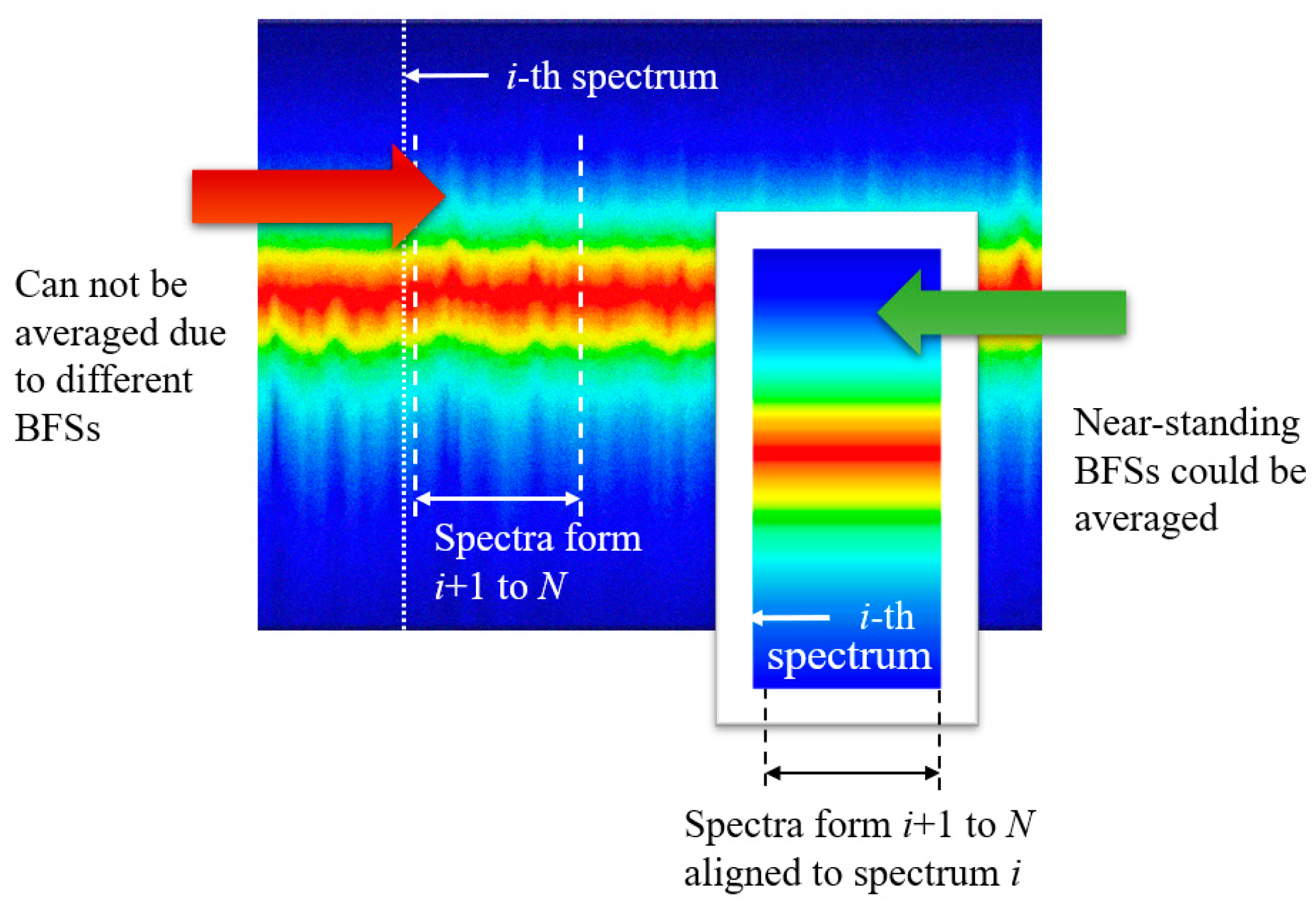
2. The Idea of the Proposed Method

The data received for processing are typical BGS, i.e., a set of scattering spectra obtained for each point of the optical sensor. These data can be easily visualized as an image (Figure 2), in which the abscissa axis is the distance, the ordinate axis is the frequency, and the color information characterizes the radiation intensity. Given that the original frequency resolution is relatively low, the method entails upsampling, which involves the generation of new pixels. In the simplest case, the color of these pixels is determined by a linear approximation based on neighboring pixels.
To calculate the BFS of spectrum i, a certain set P is selected, consisting of N consecutive spectra that will be involved in digital signal processing. This choice is made based on the computing resources and the tasks facing the researcher. How to determine the optimal value of N will be shown in the subsequent parts of this paper. It is worth noting that the set P does not contain a spectrum with the number i.
Next, the cross-correlation function (CCF) of spectrum i and spectrum i + 1, the first of the spectra of set P, is calculated. The maximum of this function determines the shift of the spectra relative to each other, at which their maximum overlap will occur. All values of spectrum number i + 1 are shifted by the value d:
d i + 1 = M a x _ j N N S i + 1 ; j   S i ; j n   ,
S i + 1 ; j = S i + 1 ; j + d i + 1 ,
where n is the argument of the CCF, Max_j is the function returning the coordinate j of the maximum value of the CCF. If the spectrum with index i + m does not fall into the set P because the end of the fiber line has been reached, then it is replaced by the spectrum with index Nm, where m is an integer value. Thus, the coordinates of the BGS maxima with numbers i and i + 1 (or Nm) become almost equal. An exact match is not achieved due to the error of the correlation method, which takes its own value for each of the spectra of set P and can even change the sign. Thereafter, all shifted BGS are normalized and added up, and the BFS value is calculated from the resulting spectrum using the LCF method.
An algorithm was developed and subsequently applied to both the simulated data and the experimental data (Figure 3) to assess the efficacy of the proposed approach.
At the outset of the calculations, two independent processing branches are established. The first of these incorporates data processing. The traditional BFS extraction method, LCF, is employed to derive the BFS 1 set. The second branch commences with resampling and continues processing according to the aforementioned algorithm (Figure 3). At the conclusion of each branch, the precision and accuracy parameters are analyzed, and the results are ultimately compared.

Description of Metrics for Comparing Algorithms

Accuracy is the average deviation of the obtained value from the true one. In the case of simulated spectra, the true value is known in advance. In contrast, in the case of experimentally obtained spectra, the true value is, in a strict sense, unknown. However, in a good approximation, the true value can be taken as equal to the value measured on a spectrum with ideal characteristics (small scanning step and high SNR) at the same fiber point.
Precision, in its classical sense, refers to the repeatability of measurement and is not directly related to the true value. However, a correction is required in the present case, as the measurements correspond to different points on the fiber. It would be erroneous to compare the obtained values without accounting for this discrepancy. Consequently, the values of the spectrum maximum frequency were selected as the initial data for calculating precision in shifted coordinate systems (i.e., when the spectral centers are combined according to the algorithm described above).

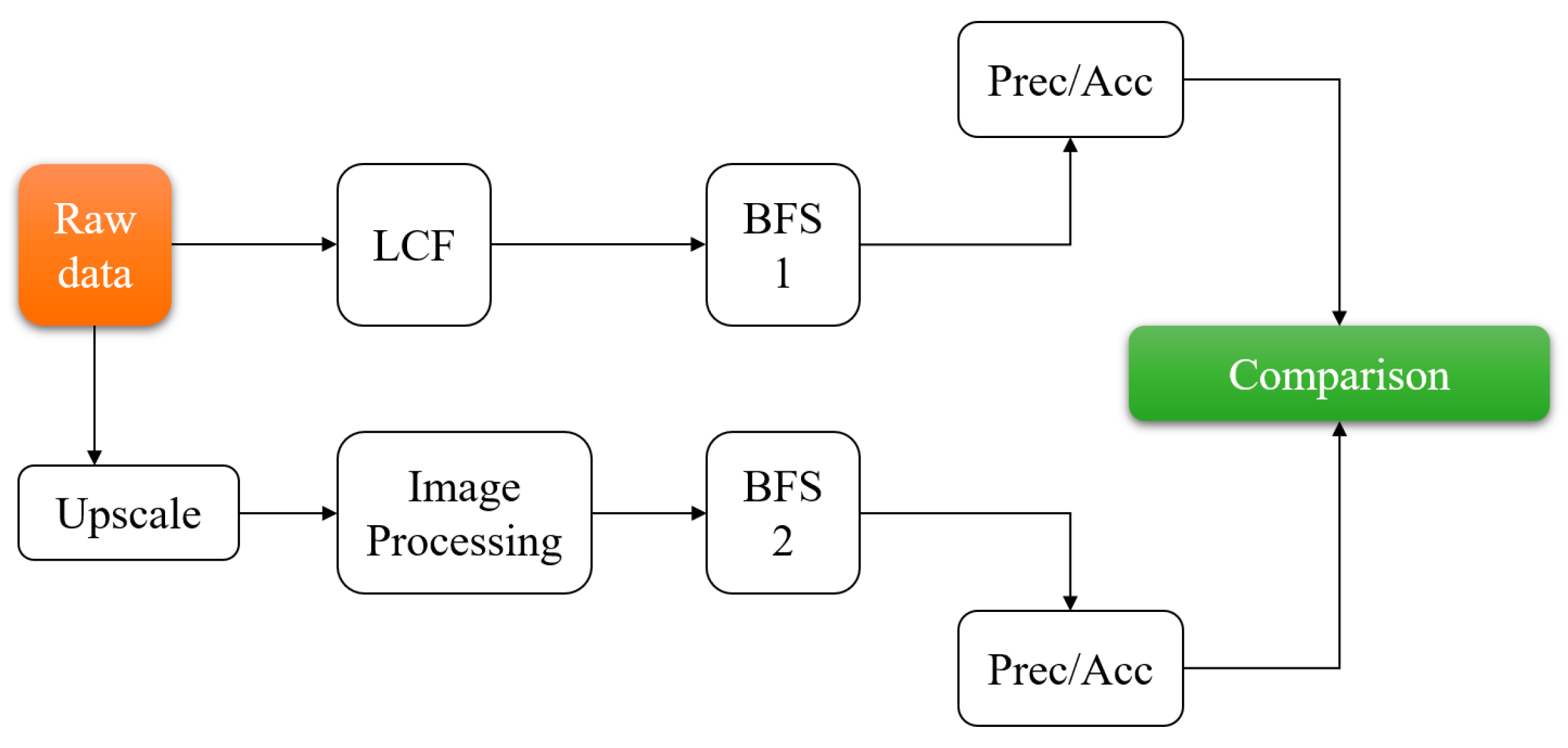
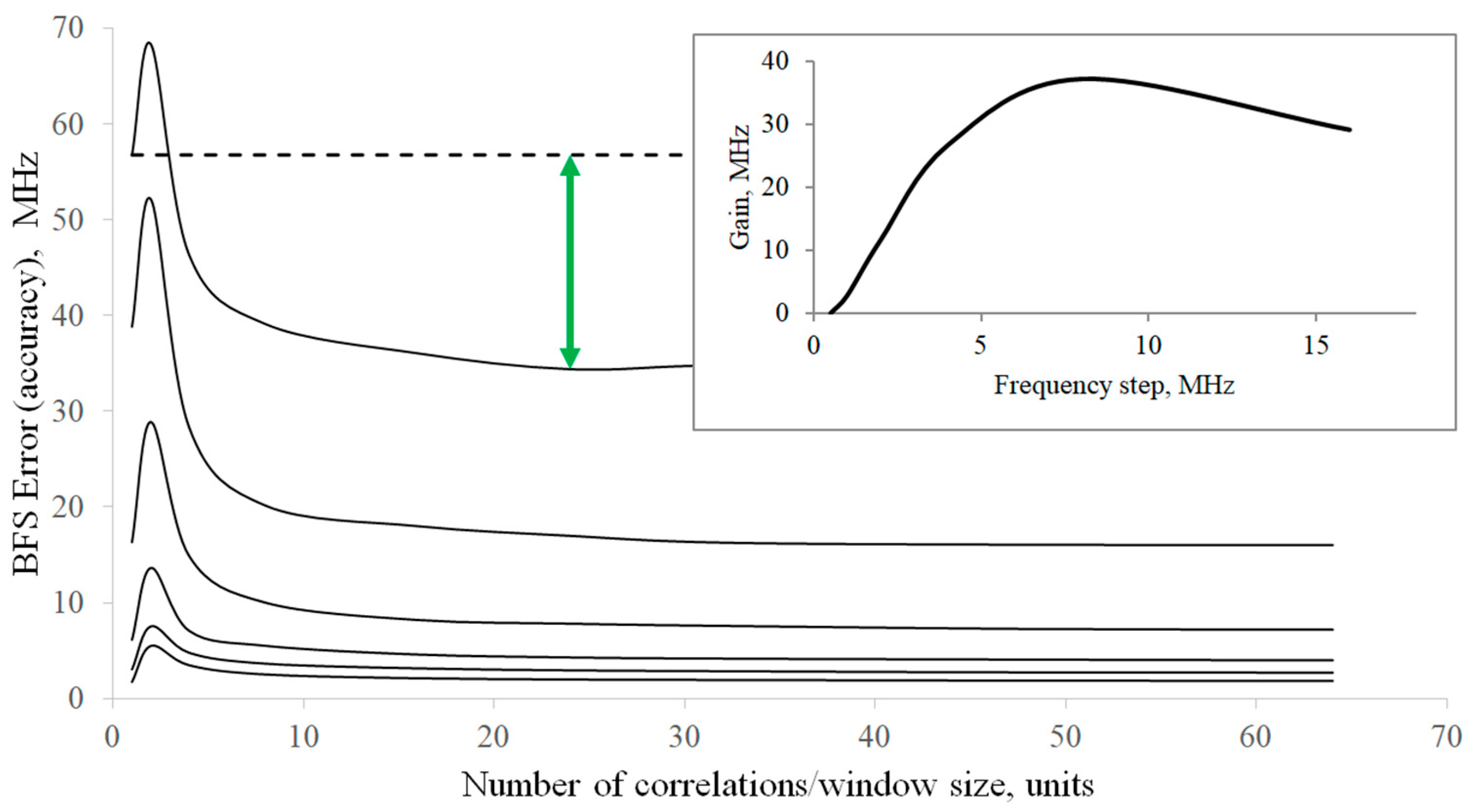
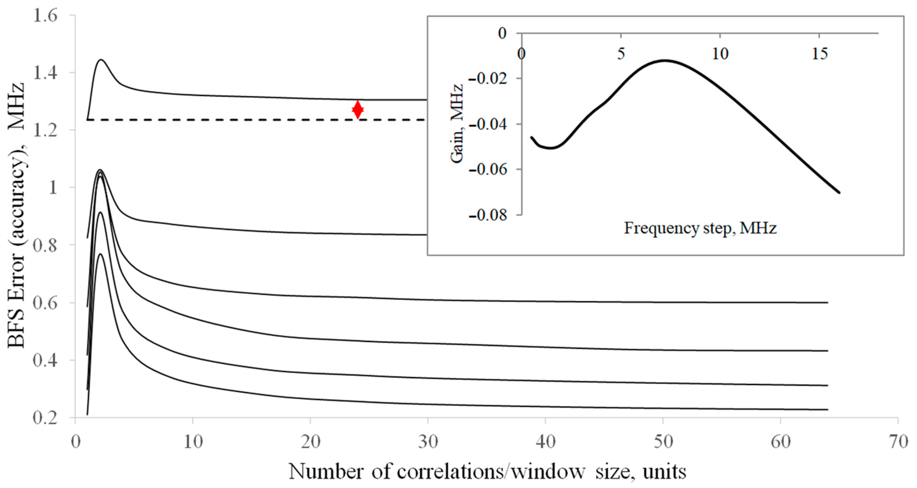
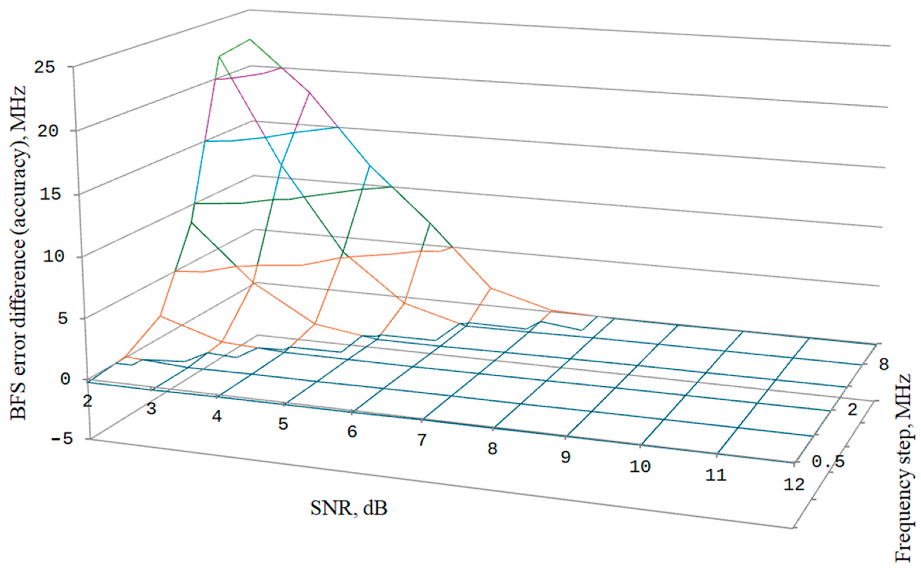
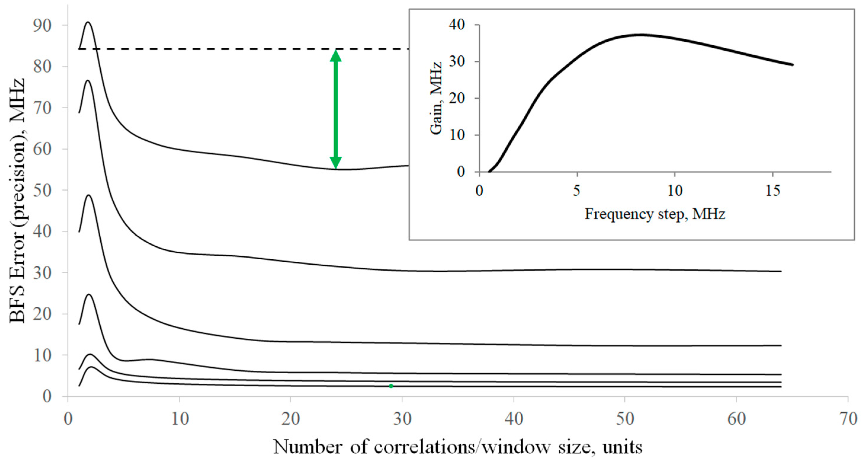
3. The Simulation and Its Results

Six sets of Brillouin spectra were simulated using a computer experiment according to Equation (1) to validate the proposed method. Each set imitated a spectrum matrix measured using a BOTDA with a certain scanning step: 0.5, 1, 2, 4, 8, and 16 MHz. For each scanning step, a generated matrix had a fixed signal-to-noise ratio (SNR) of spectra, ranging from 2 to 12 dB, with a step of 1 dB. Given that these spectra have been artificially simulated, the true BFS for each spectrum is known in advance.
Figure 4 illustrates the dependence of the error (accuracy) in determining the position of the BGS maximum on the number of spectra involved in the averaging procedure for modeled spectra with an SNR of 2 dB.
The upper curve corresponds to the results of spectra with a frequency step of 16 MHz processing. The subsequent curves, from top to bottom, depict the results of processing spectra with steps of 8, 4, 2, 1, and 0.5 MHz, respectively. The procedure for determining the gain in accuracy is illustrated for a step of 16 MHz. The dashed line depicts the error in determining BFS by the classical LCF method without averaging neighboring spectra. The green arrow represents the difference between the BFS extraction errors by the proposed method and LCF for 24 spectra involved in the correlation process. The number of correlation spectra was chosen to reduce the processing time while maintaining high accuracy. The final dependence of the gain on the frequency step is shown in the inset, which is calculated with the formula:
= E L C F E I P ,
where is the gain in accuracy of BFS extraction; E L C F is the BFS extraction error of the LCF method;   E I P is the BFS extraction error of the IP method.
As illustrated in Figure 4, the proposed algorithm yields superior outcomes compared to the LCF method, starting with eight averaged spectra. At approximately 20 spectra, the gain reaches its maximum value, and with an increase in the number of spectra, the gain remains relatively constant. Figure 5 presents similar results, but when processing spectra with an SNR of 11 dB. It can be observed that the algorithm approaches the accuracy of the classical LCF with a large number of averaged spectra yet does not outpace it.
Figure 6 illustrates the discrepancy in the efficacy of the proposed algorithm and the LCF method. For the sake of clarity, the outcomes are presented as a surface, and the higher the point on the surface, the greater the gain of the proposed algorithm.
As illustrated in Figure 6, the algorithm demonstrates a clear advantage over LCF in the context of low SNR and coarse scanning steps over the spectrum.
Precision outcomes for the second selected metric are similar (Figure 7). The algorithm outperforms LCF at low SNR and large scanning steps. The optimal value of the averaged spectra is approximately 20.

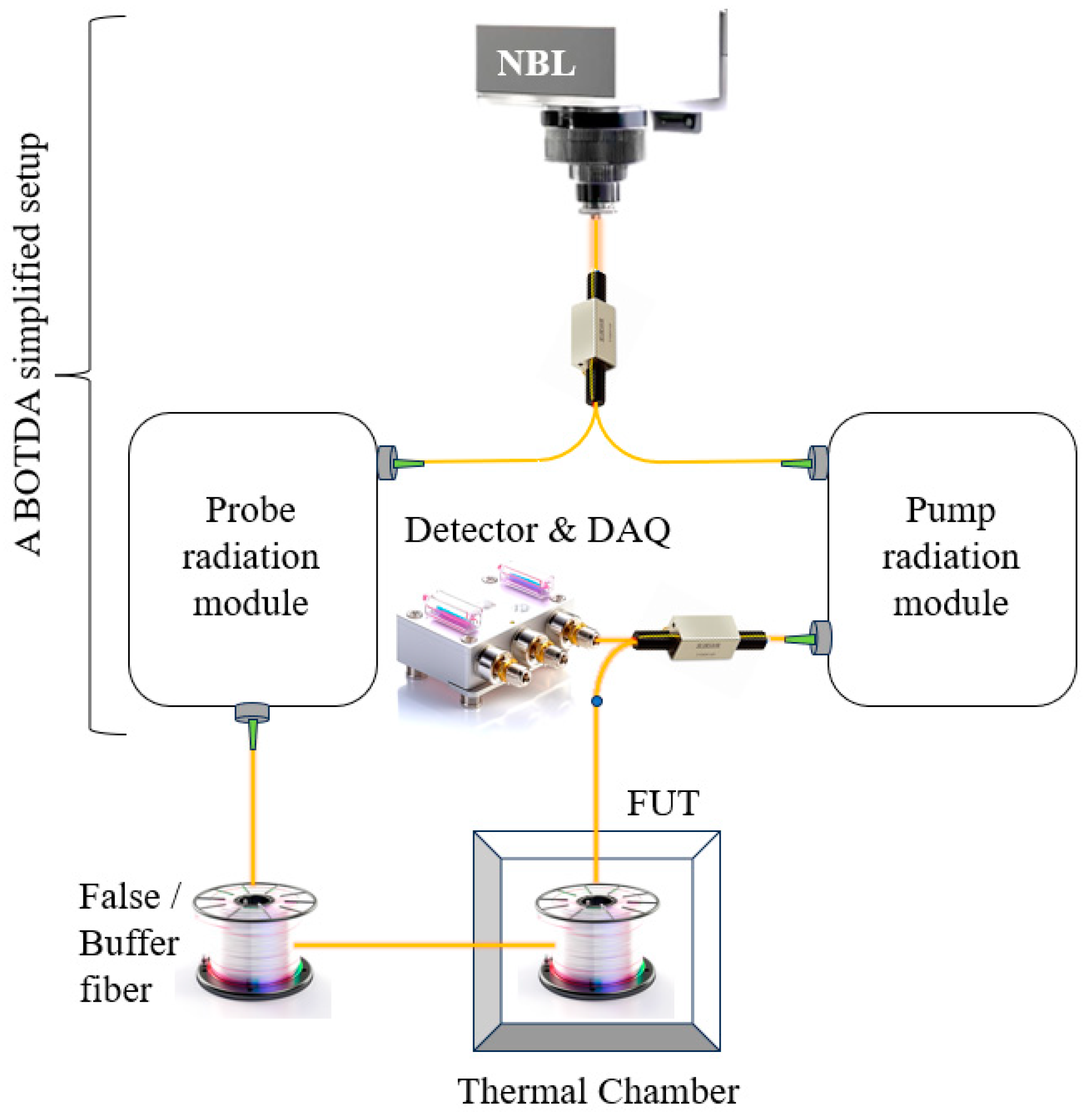
4. The Experiment and Its Results

A commercial Brillouin analyzer and standard telecommunication optical fiber SMF-28e were used for the experiments. The optical fiber on a split spool (free winding) was placed in a thermal chamber, where the temperature was maintained at 25 °C during the experiment to eliminate the influence of temperature variations in the laboratory on the experimental data.
Figure 8 shows the experimental setup, including a simplified installation of BOTDA. In this experiment, the DiTeSt 202 STA-R instrument from Omnisens (Morges, Switzerland) was employed. Furthermore, the results obtained with this system have allowed us to compare the outcomes of our previous studies, thereby facilitating the assessment of the efficacy of the proposed methodologies under identical conditions. A typical instrument of this type comprises a pair of main modules: a pump and probe modules. The initial radiation for both modules is typically generated by a narrow-bandwidth laser operating at a wavelength of 1550 nm in continuous mode. The pump module transforms continuous radiation into pulsed radiation through modulation and subsequently amplifies it through a two-stage erbium amplification process. As a consequence of this configuration, the pump module generates rectangular pulses with a duration of approximately tens of nanoseconds, which are then fed to the sensor fiber. The duration of the pause between pulses is typically characterized by microseconds, which is due to the pulse’s time travel through the length of the sensor. In this case, we used pulses with a duration of 10 nanoseconds, which enabled the system to obtain traces with a resolution of 1 m. Additionally, the system shifts this radiation in frequency. We used measurements with a fixed frequency shift of 1 MHz and then performed frequency downsampling to emulate a coarse scanning step. Pigtails equipped with E2000/APC connectors (NTSS, Kostroma, Russia) were welded to the ends of the optical fiber under study using an Ilsintech KF4 arc splicing machine (Ilsintech, DaeJeon City, Republic of Korea). Subsequent to this, the optical fiber under study was placed on a split spool in an Espec MC711, (Espec, Osaka, Japan) thermal chamber for thermostatting. The pressure of individual fibers on each other, axial twisting, and, consequently, undesirable changes in signal polarization and attenuation coefficient were prevented by using a split spool and careful laying of the fiber in the chamber. A temperature close to room temperature of 25 °C was chosen for thermostatting. Once the temperature of the coil and fiber stabilized, cyclic measurements were initiated. The rationale behind the deliberate disabling of the automatic frequency scanning step selection for this study is the need to calculate a discrete correlation function.
The frequency variation range of 10,700 to 10,900 MHz was selected based on the characteristic BFS variations of this fiber type under normal conditions.
Over the 10-h experimental period, 105 measurements were obtained and subsequently transformed into images with varying signal-to-noise ratios by modifying the BGS sample size for averaging.
The signal-to-noise ratio was calculated using the LCF method with subsequent subtraction of the Lorentzian fitted curve from the signal. The spectrum intensity at the maximum point of the Lorentzian curve was taken as the signal level, and the average signal value after its subtraction was taken as the noise level. Based on these two obtained values, the signal-to-noise ratio was calculated. The number of spectra accumulated for averaging by the BGS device varied from 103 to 107, allowing for the acquisition of spectra with varying SNRs.
It is essential to compare the processed values with a standard to assess the efficacy of the employed methods. All spectra obtained for a given temperature (in this case, all 108) were averaged to obtain an accurate standard value for the quantity under study, and reference BFS values were calculated using the LCF method.
The sensor line was 1 km long. It should be noted that averaging was performed for each spatial coordinate separately, as any optical fiber, even those produced by well-established VAD/OVD methods, still exhibits some BFS variation along its length.
Figure 9 and Figure 10 illustrate the relationship between the error/repeatability in determining BFS and the number of experimentally measured spectra involved in the processing. In this instance, the spectra obtained with the accumulation of 103 were subjected to processing. Consequently, the SNR, as determined by the aforementioned method, was found to be 2–3 dB.
The obtained results are in good agreement with the simulation. The proposed method outperforms LCF in both metrics. The optimal number of spectra for processing is approximately 16. For spectra with an accumulation of 5 × 10⁴ (which corresponds to an SNR of approximately 11 dB), similar dependencies are shown in Figure 11 and Figure 12. In this instance, the advantage is only achieved with large scanning steps. With a scanning step of less than 2 MHz, the proposed algorithm is outperformed by LCF.
Finally, Figure 13 illustrates the discrepancy in the efficacy of the proposed algorithm and the LCF method for experimental data.

5. Discussion

The accuracy of BFS extraction from the spectrum is influenced by several factors, including the scanning step size and signal-to-noise ratio (SNR). Regardless of the algorithm employed, the error tends to decrease with increasing SNR and increase with increasing scanning step [49]. However, another crucial factor is the shape of the spectrum, and in this regard, the algorithms exhibit markedly disparate behaviors. LCF is considerably more susceptible to spectrum defects than correlation [50] and artificial intelligence [51] algorithms.
As the final step of the proposed algorithm is still LCF, it is necessary to analyze the impact of the preliminary stages of processing (resampling and averaging with neighboring spectra) on the spectrum itself. A reduction in the spectrum’s discreteness is a consequence of the algorithm itself, and it is logical to expect an increase in the SNR due to the averaging effect during processing. However, what happens to the shape?
When each spectrum of set P is shifted (unless the position of its maximum coincides with the position of the maximum of the measured spectrum), a negative edge defect is introduced. It is illustrated in Figure 14a shows the first spectrum, Figure 14b demonstrates the second. It is necessary to shift the second spectrum to the left to align them by the maximum position, while the extreme right values are filled with zeros. Figure 14c shows the final spectrum, obtained as a half-sum of the original first and shifted second spectra. The spectrum has a kink (shown in the inset on an enlarged scale for clarity). Due to the edge effect, the shape of the spectrum has been distorted, and asymmetry has appeared. The negative impact of spectrum asymmetry on LCF accuracy was previously observed by the authors in [52].
We think this is the reason for the increase in the BFS extraction error when a small number of spectra are involved in the processing compared to pure LCF (Figure 4, Figure 5, Figure 9, and Figure 10). The negative effect of the distorted spectrum shape is believed to prevail over the positive effect of reducing discreteness and increasing SNR. Moreover, if set P consists of only one spectrum, the averaged spectrum will be obviously asymmetric (as in Figure 14), with zero values added only at one edge of the spectrum. Consequently, the negative effect will be dramatic, as is evident in the obtained graphs. However, with a greater number of spectra involved, the positive effects become more pronounced, and the BFS extraction error fades.
In our opinion, the same thing explains the larger jump in the graph upwards in the initial section when processing the model spectra (Figure 5 and Figure 6) than the experimental data (Figure 11 and Figure 12). This can be attributed to the smaller dispersion of the BFS value along the fiber in the experiment than in the simulation. Consequently, a smaller shift was required to align the experimental spectra, and the introduced deformation of the spectrum shape was of a smaller nature. Under other experimental conditions (for example, without using a thermal chamber), the quantitative agreement between the results of processing the experimental and simulated spectra would have been higher.

6. Conclusions

This paper successfully demonstrates the efficacy of two-dimensional digital signal processing based on spectra alignment in improving the parameters of the original BGS. This leads to a gain in the accuracy and precision of frequency shift detection at coarse frequency scanning steps and low signal-to-noise ratios. This approach allows for an increase in the length of the fiber sensor and in measurement speed. However, the method has its own drawbacks. The most obvious of these is the high requirement for computing resources. In our opinion, this problem is significant since the method is adapted for fast measurements (coarse frequency step), but in fact, the measurement results can be obtained at this stage only in the post-processing mode.
Based on this, it is possible to outline the front of the following works aimed at eliminating this drawback:
  • It is imperative to optimize the algorithm to eliminate duplicate operations.
  • Of particular interest is the alignment of spectra through the use of artificial intelligence rather than the traditional approach of calculating the correlation function.
  • The calculation function is to be transferred to the hardware part of the device.
It is also important to note that the method has parameters that can be varied. The most significant of them is the number of spectra that fall within the sliding window and, as a result, are subject to alignment. Our findings indicate that the relationship between this value and the accuracy of determining the frequency shift at different signal-to-noise ratios and frequency scanning steps is not straightforward. This was confirmed both in modeling and in the experiment. It is our hope that optimization of the calculations will facilitate more in-depth research in the near future.
With regard to potential applications, the algorithm can already be used to process signals from reflectometers and analyzers that use a laser source with self-scanning in frequency. Furthermore, a significant improvement in accuracy will be observed when monitoring lines several tens of kilometers long at the far end of the fiber.
The method is of particular interest for studying optical fibers with high losses, including various special fibers such as photonic crystals, active fibers, and others.
In our opinion, the potential for using the sensor in extreme conditions, where temperature or deformation (including unpredictable bends) increases the attenuation coefficient of the optical signal in the fiber, which leads to a decrease in SNR and data not falling within the dynamic range of the system, is worthy of further investigation. The utilization of the aforementioned methodology will enhance the functionality of testing units and components, as well as the capacity of entire devices created using new technologies and/or new materials.

Author Contributions

Conceptualization, supervision, writing—Y.K.; validation, formal analysis, writing—F.B.; software, experiment, visualization—A.K. All authors have read and agreed to the published version of the manuscript.

Funding

The authors acknowledge the financial support of the Ministry of Education and Science of the Russian Federation (Agreement No. 075-15-2022-329 of 21 April 2022).

Data Availability Statement

The experimental data presented in this study are available upon reasonable request from the corresponding author.

Conflicts of Interest

The authors declare no conflicts of interest.

References

  1. Song, Y.; Tian, H.; Jia, Z.; Chen, W.; Zhang, W.; Wang, C.; Zhou, T.; Li, L.; Hong, D.; Wang, Y.; et al. Distributed Partial Discharge Acoustic Signal Detection and Localization Technology for GIL with Built-in Fiber Optics. J. Light. Technol. 2024, 42, 5068–5076. [Google Scholar] [CrossRef]
  2. Kovalenko, D.; Sodnomay, A.; Alekseenko, Z.; Shelemba, I.; Lobach, I.; Firstov, S.; Melkumov, M. Loss-Compensated Dual-Source Raman-DTS with Bismuth- and Erbium-doped Fiber Amplifiers. In Optical Fiber Sensors Conference 2020 Special Edition; Paper T3.44; Cranch, G., Wang, A., Digonnet, M., Dragic, P., Eds.; OSA Technical Digest, Optica Publishing Group: Washington, DC, USA, 2020. [Google Scholar]
  3. Matveenko, V.P.; Serovaev, G.S.; Kosheleva, N.A.; Galkina, E.B. Investigation of fiber Bragg grating’s spectrum response to strain gradient. Procedia Struct. Integr. 2024, 54, 218–224. [Google Scholar] [CrossRef]
  4. Fu, C.; Xiao, S.; Meng, Y.; Shan, R.; Liang, W.; Zhong, H.; Liao, C.; Yin, X.; Wang, Y. OFDR shape sensor based on a femtosecond-laser-inscribed weak fiber Bragg grating array in a multicore fiber. Opt. Lett. 2024, 49, 1273–1276. [Google Scholar] [CrossRef]
  5. Höttges, A.; Rabaiotti, C.; Facchini, M. A Novel Distributed Fiber-Optic Hydrostatic Pressure Sensor for Dike Safety Monitoring. IEEE Sens. J. 2023, 23, 28942–28953. [Google Scholar] [CrossRef]
  6. Zhang, W.; Ni, X.; Wang, J.; Ai, F.; Luo, Y.; Yan, Z.; Liu, D.; Sun, Q. Microstructured Optical Fiber Based Distributed Sensor for In Vivo Pressure Detection. J. Light. Technol. 2019, 37, 1865–1872. [Google Scholar] [CrossRef]
  7. Chen, C.; Zhao, Z.; Lin, Z.; Yao, Y.; Xiong, Y.; Tong, W.; Tang, M. Distributed twist sensing using frequency-scanning φ-OTDR in a spun fiber. Opt. Express 2023, 31, 17809–17819. [Google Scholar] [CrossRef]
  8. Gritsenko, T.V.; Chesnokov, G.Y.; Koshelev, K.I.; Khan, R.I.; Stepanov, K.V.; Valba, O.V.; Chernutsky, A.O.; Svelto, C.; Zhirnov, A.A.; Pnev, A.B.; et al. Optical Fiber Sensor for Real-Time Monitoring of Industrial Structures and Application to Urban Telecommunication Networks. In Proceedings of the 2023 IEEE International Conference on Metrology for eXtended Reality, Artificial Intelligence and Neural Engineering (MetroXRAINE), Milano, Italy, 25–27 October 2023; pp. 383–388. [Google Scholar] [CrossRef]
  9. Bengalskii, D.M.; Kharasov, D.R.; Fomiryakov, E.A.; Nikitin, S.P.; Nanii, O.E.; Treshchikov, V.N. Characterization of Laser Frequency Stability by Using Phase-Sensitive Optical Time-Domain Reflectometry. Photonics 2023, 10, 1234. [Google Scholar] [CrossRef]
  10. Yang, D.; Denney, T.; Bello, O.; Lazarus, S.; Vettical, C. Enabling Real-Time Distributed Sensor Data for Broader Use by the Big Data Infrastructures. Presented at the SPE Intelligent Energy International Conference and Exhibition, Aberdeen, Scotland, UK, 6 September 2016. [Google Scholar] [CrossRef]
  11. Sharma, J.; Santos, O.L.A.; Feo, G.; Ogunsanwo, O.; Williams, W. Well-scale multiphase flow characterization and validation using distributed fiber-optic sensors for gas kick monitoring. Opt. Express 2020, 28, 38773–38787. [Google Scholar] [CrossRef]
  12. Leite, T.M.; Freitas, C.; Magalhães, R.; da Silva, A.F.; Alves, J.R.; Viana, J.C.; Delgado, I. Decoupling of Temperature and Strain Effects on Optical Fiber-Based Measurements of Thermomechanical Loaded Printed Circuit Board Assemblies. Sensors 2023, 23, 8565. [Google Scholar] [CrossRef]
  13. Soga, K.; Luo, L. Distributed fiber optics sensors for civil engineering infrastructure sensing. J. Struct. Integr. Maint. 2018, 3, 1–21. [Google Scholar] [CrossRef]
  14. Franciscangelis, C.; Margulis, W.; Floridia, C.; Rosolem, J.B.; Salgado, F.C.; Nyman, T.; Petersson, M.; Hallander, P.; Hällstrom, S.; Söderquist, I.; et al. Vibration measurement on composite material with embedded optical fiber based on phase-OTDR. In Proceedings of the SPIE 10168, Sensors and Smart Structures Technologies for Civil, Mechanical, and Aerospace Systems 2017, Portland, OR, USA, 12 April 2017; p. 101683Q. [Google Scholar] [CrossRef]
  15. Stepanov, K.V.; Zhirnov, A.A.; Sazonkin, S.G.; Pnev, A.B.; Bobrov, A.N.; Yagodnikov, D.A. Non-Invasive Acoustic Monitoring of Gas Turbine Units by Fiber Optic Sensors. Sensors 2022, 22, 4781. [Google Scholar] [CrossRef] [PubMed]
  16. Li, Y.; Wang, L.; Fan, H. Influence of laser wavelength instability, polarization fading and phase fluctuation on local heterodyne detection wavelength scanning BOTDR. Optoelectron. Lett. 2023, 19, 200–204. [Google Scholar] [CrossRef]
  17. Li, M.; Xu, T.; Wang, S.; Hu, W.; Jiang, J.; Liu, T. Probe pulse design in Brillouin optical time domain reflectometry. IET Optoelectron. 2022, 16, 238–252. [Google Scholar] [CrossRef]
  18. Almoosa, A.S.K.; Zan, M.S.D.; Ibrahim, M.F.; Tanaka, Y.; Hamzah, A.E.; Arsad, N. Fast and accurate Brillouin frequency shift extraction in Brillouin optical time domain reflectometry (BOTDR) distributed fiber sensor by using ensemble machine learning algorithm. J. Phys. Conf. Ser. 2022, 2411, 012012. [Google Scholar] [CrossRef]
  19. Fu, Y.; Zhu, R.; Han, B.; Wu, H.; Rao, Y.-J.; Lu, C.; Wang, Z. 175-km Repeaterless BOTDA with Hybrid High-Order Random Fiber Laser Amplification. J. Light. Technol. 2019, 37, 4680–4686. [Google Scholar] [CrossRef]
  20. Peng, J.; Wang, T.; Zhang, Q.; Ge, X.; Zhu, Y.; Zhang, Y.; Zhang, J.; Li, J.; Zhang, M. High Spatial Resolution BOTDA Based on Deconvolution and All Phase Digital Filtering. IEEE Sens. J. 2024, 24, 10024–10030. [Google Scholar] [CrossRef]
  21. Hamzah, A.E.; Bakar, A.A.A.; Fadhel, M.M.; Sapiee, N.M.; Elgaud, M.M.; Hamzah, M.E.; Almoosa, A.S.K.; Naim, N.F.; Mokhtar, M.H.H.; Ali, S.H.M.; et al. Advancing the measurement speed and accuracy of conventional BOTDA fiber sensor systems via SoC data acquisition. Opt. Fiber Technol. 2024, 84, 103712. [Google Scholar] [CrossRef]
  22. Bogachkov, I.V.; Gorlov, N.I. Research of the Optical Fibers Structure Influence on the Acousto-Optic Interaction Characteristics and the Brillouin Scattering Spectrum Profile. J. Phys. Conf. Ser. 2022, 2182, 012088. [Google Scholar] [CrossRef]
  23. Krivosheev, A.I.; Barkov, F.L.; Konstantinov, Y.A.; Belokrylov, M.E. State-of-the-Art Methods for Determining the Frequency Shift of Brillouin Scattering in Fiber-Optic Metrology and Sensing. Instrum. Exp. Tech. 2022, 65, 687–710. [Google Scholar] [CrossRef]
  24. Poddubrovskii, N.R.; Lobach, I.A.; Kablukov, S.I. Microwave-free BOTDA based on a continuous-wave self-sweeping laser. Opt. Lett. 2024, 49, 282–285. [Google Scholar] [CrossRef] [PubMed]
  25. Lobach, I.A.; Kablukov, S.I.; Melkumov, M.A.; Khopin, V.F.; Babin, S.A.; Dianov, E.M. Single-frequency Bismuth-doped fiber laser with quasi-continuous self-sweeping. Opt. Express 2015, 23, 24833–24842. [Google Scholar] [CrossRef]
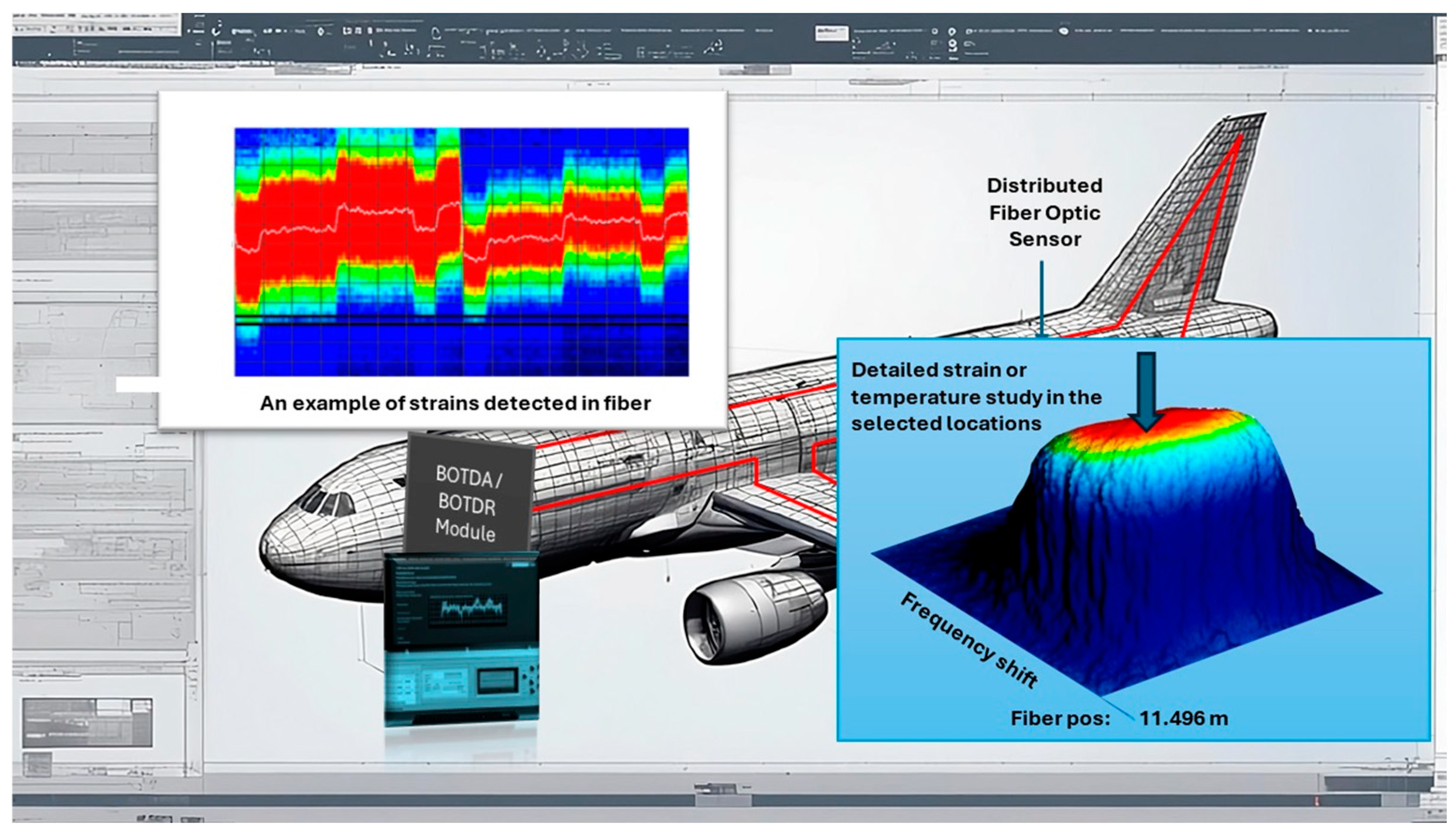
  26. Yari, T.; Nagai, K.; Takeda, N. Aircraft structural-health monitoring using optical fiber distributed BOTDR sensors. Adv. Compos. Mater. 2004, 13, 17–26. [Google Scholar] [CrossRef]
  27. Shimizu, T.; Yari, T.; Nagai, K.; Takeda, N. Strain measurement using a Brillouin optical time domain reflectometer for development of aircraft structure health monitoring system. In Proceedings of the SPIE 4335, Advanced Nondestructive Evaluation for Structural and Biological Health Monitoring, Newport Beach, CA, USA, 24 July 2001. [Google Scholar] [CrossRef]
  28. Sante, D.; Fibre, R. Optic Sensors for Structural Health Monitoring of Aircraft Composite Structures: Recent Advances and Applications. Sensors 2015, 15, 18666–18713. [Google Scholar] [CrossRef]
  29. Marquardt, D.W. An Algorithm for Least-Squares Estimation of Nonlinear Parameters. J. Soc. Indust. Appl. Math. 1963, 11, 431–441. [Google Scholar] [CrossRef]
  30. Levenberg, K. A method for the solution of certain non-linear problems in least squares. J. Q. Appl. Math. 1944, 2, 164–168. [Google Scholar] [CrossRef]
  31. Lourakis, M.L.A.; Argyros, A.A. Is Levenberg-Marquardt the most efficient optimization algorithm for implementing bundle adjustment? In Proceedings of the Tenth IEEE International Conference on Computer Vision (ICCV’05) Volume 1, Beijing, China, 17–21 October 2005; Volume 2, pp. 1526–1531. [Google Scholar] [CrossRef]
  32. Farahani, M.A.; Castillo-Guerra, E.; Colpitts, B.G. A Detailed Evaluation of the Correlation-Based Method Used for Estimation of the Brillouin Frequency Shift in BOTDA Sensors. IEEE Sens. J. 2013, 13, 4589–4598. [Google Scholar] [CrossRef]
  33. Barkov, F.L.; Konstantinov, Y.A.; Krivosheev, A.I. A Novel Method of Spectra Processing for Brillouin Optical Time Domain Reflectometry. Fibers 2020, 8, 60. [Google Scholar] [CrossRef]
  34. Farahani, M.A.; Colpitts, B.G.; Castillo-Guerra, E. Reduction of measurement time in BOTDA sensors using wavelet shrinkage. In Proceedings of the SPIE 7753, 21st International Conference on Optical Fiber Sensors, Ottawa, ON, Canada, 17 May 2011; p. 77532E. [Google Scholar] [CrossRef]
  35. Wang, B.; Wang, L.; Guo, N.; Zhao, Z.; Yu, C.; Lu, C. Deep neural networks assisted BOTDA for simultaneous temperature and strain measurement with enhanced accuracy. Opt. Express 2019, 27, 2530–2543. [Google Scholar] [CrossRef]
  36. Ruiz-Lombera, R.; Fuentes, A.; Rodriguez-Cobo, L.; Lopez-Higuera, J.M.; Mirapeix, J. Simultaneous Temperature and Strain Discrimination in a Conventional BOTDA via Artificial Neural Networks. J. Light. Technol. 2018, 36, 2114–2121. [Google Scholar] [CrossRef]
  37. Qu, S.; Qin, Z.; Xu, Y.; Cong, Z.; Wang, Z.; Liu, Z. Improvement of Strain Measurement Range via Image Processing Methods in OFDR System. J. Light. Technol. 2021, 39, 6340–6347. [Google Scholar] [CrossRef]
  38. Zhao, S.; Cui, J.; Wu, Z.; Tan, J. Accuracy improvement in OFDR-based distributed sensing system by image processing. Opt. Lasers Eng. 2020, 124, 105824. [Google Scholar] [CrossRef]
  39. Turov, A.T.; Barkov, F.L.; Konstantinov, Y.A.; Korobko, D.A.; Lopez-Mercado, C.A.; Fotiadi, A.A. Activation Function Dynamic Averaging as a Technique for Nonlinear 2D Data Denoising in Distributed Acoustic Sensors. Algorithms 2023, 16, 440. [Google Scholar] [CrossRef]
  40. Qian, X.; Wang, Z.; Sun, W.; Zhang, B.; He, Q.; Zhang, L.; Wu, H.; Rao, Y. Long-range BOTDA denoising with multi-threshold 2D discrete wavelet. In Proceedings of the Asia Pacific Optical Sensors Conference, Shanghai, China, 11–14 October 2016; OSA Technical Digest (online); paper W4A.24. Optica Publishing Group: Washington, DC, USA, 2016. [Google Scholar]
  41. Soto, M.A.; Ramírez, J.A.; Thévenaz, L. Intensifying the response of distributed optical fibre sensors using 2D and 3D image restoration. Nat. Commun. 2016, 7, 10870. [Google Scholar] [CrossRef] [PubMed]
  42. Qian, X.; Wang, Z.; Wang, S.; Xue, N.; Sun, W.; Zhang, L.; Zhang, B.; Rao, Y. 157km BOTDA with pulse coding and image processing. In Proceedings of the SPIE 9916, Sixth European Workshop on Optical Fibre Sensors, Limerick, Ireland, 30 May 2016; p. 99162S. [Google Scholar] [CrossRef]
  43. Soto, M.A.; Ramírez, J.A.; Thévenaz, L. Optimizing Image Denoising for Long-Range Brillouin Distributed Fiber Sensing. J. Light. Technol. 2018, 36, 1168–1177. [Google Scholar] [CrossRef]
  44. Li, B.; Jiang, N.; Han, X. Denoising of Brillouin Gain Spectrum Images for Improved Dynamic Measurements of BOTDR. IEEE Photon-J. 2023, 15, 6801808. [Google Scholar] [CrossRef]
  45. Hu, Y.; Shang, Q. Performance Enhancement of BOTDA Based on the Image Super-Resolution Reconstruction. IEEE Sens. J. 2021, 22, 3397–3404. [Google Scholar] [CrossRef]
  46. Zheng, H.; Zhang, J.; Wu, H.; Guo, N.; Zhu, T. Single shot OCC-BOTDA based on polarization diversity and image denoising. Opt. Lasers Eng. 2021, 137, 106368. [Google Scholar] [CrossRef]
  47. Wang, Q.; Bai, Q.; Liu, Y.; Wang, J.; Wang, Y.; Jin, B. SNR Enhancement for BOTDR With Spatial-Adaptive Image Denoising Method. J. Light. Technol. 2023, 41, 2562–2571. [Google Scholar] [CrossRef]
  48. Hamzah, A.E.; Zan, M.S.D.; Hamzah, M.E.; Fadhel, M.M.; Sapiee, N.M.; Bakar, A.A.A. Fast and Accurate Measurement in BOTDA Fiber Sensor Through the Application of Filtering Techniques in Frequency and Time Domains. IEEE Sens. J. 2024, 24, 4531–4541. [Google Scholar] [CrossRef]
  49. Soto, M.A.; Thévenaz, L. Modeling and evaluating the performance of Brillouin distributed optical fiber sensors. Opt. Express 2013, 21, 31347–31366. [Google Scholar] [CrossRef]
  50. Krivosheev, A.I.; Konstantinov, Y.A.; Barkov, F.L.; Pervadchuk, V.P. Comparative Analysis of the Brillouin Frequency Shift Determining Accuracy in Extremely Noised Spectra by Various Correlation Methods. Instrum. Exp. Tech. 2021, 64, 715–719. [Google Scholar] [CrossRef]
  51. Karapanagiotis, C.; Krebber, K. Machine Learning Approaches in Brillouin Distributed Fiber Optic Sensors. Sensors 2023, 23, 6187. [Google Scholar] [CrossRef] [PubMed]
  52. Barkov, F.L.; Krivosheev, A.I.; Konstantinov, Y.A.; Davydov, A.R. A Refinement of Backward Correlation Technique for Precise Brillouin Frequency Shift Extraction. Fibers 2023, 11, 51. [Google Scholar] [CrossRef]
Figure 1. An example of the BOTDA/BOTDR type systems applications in monitoring the condition of a civil aircraft [26,27,28].
Algorithms 17 00365 g001
Figure 2. The principle of the proposed method.
Algorithms 17 00365 g002
Figure 3. Algorithm for checking the efficiency of the method.
Algorithms 17 00365 g003
Figure 4. Dependences of the BFS extraction accuracy on the number of averaged spectra for spectra with SNR = 2 dB. Individual curves correspond to different scanning steps (16, 8, 4, 2, 1, and 0.5 MHz from top to bottom). Green arrow shows gain in BFS extraction accuracy. Inset: BFS extraction accuracy gain as a function of frequency step.
Algorithms 17 00365 g004
Figure 5. Dependence of the BFS extraction accuracy on the number of averaged spectra for spectra with SNR=11 dBm. Red arrow shows loss in BFS extraction accuracy. Inset: BFS extraction accuracy gain as a function of the scan step.
Algorithms 17 00365 g005
Figure 6. Dependence of the gain/loss in the accuracy of determining the BFS of the presented algorithm over LCF when processing the simulated spectra.
Algorithms 17 00365 g006
Figure 7. Dependence of the BFS extraction precision on the number of averaged spectra for spectra with SNR = 2 dBm. Green arrow shows gain in BFS extraction accuracy. Inset: BFS extraction precision gain as a function of the scan step.
Algorithms 17 00365 g007
Figure 8. An experimental setup for obtaining BGS includes the following components: FUT (fiber under test), DAQ (digital acquisition), and NBL (narrow bandwidth laser).
Algorithms 17 00365 g008
Figure 9. Dependence of the BFS extraction accuracy on the number of averaged spectra for experimental data with low SNR. Green arrow shows gain in BFS extraction accuracy. Inset: dependence of the gain in BFS extraction accuracy on the scanning step.
Algorithms 17 00365 g009
Figure 10. Dependence of the BFS extraction precision on the number of averaged spectra for experimental data with low SNR. Green arrow shows gain in BFS extraction accuracy. Inset: dependence of the gain in precision on the scanning step.
Algorithms 17 00365 g010
Figure 11. Dependence of the BFS extraction accuracy on the number of averaged spectra for experimental data with high SNR. Green arrow shows gain in BFS extraction accuracy. Inset: dependence of the gain in BFS extraction accuracy on the scanning step.
Algorithms 17 00365 g011
Figure 12. Dependence of the BFS extraction precision number of averaged spectra for experimental data with high SNR. Green arrow shows gain in BFS extraction accuracy. Inset: dependence of the gain in BFS extraction precision on the scanning step.
Algorithms 17 00365 g012
Figure 13. Dependence of the gain/loss in the accuracy of determining the BFS of the presented algorithm over LCF when processing the spectra obtained in the experiment.
Algorithms 17 00365 g013
Figure 14. Illustration of the influence of the algorithm used on the spectrum shape: (a)—original spectrum; (b)—additional spectrum; and (c)—the result of averaging two spectra, the inset shows a close-up of the kink.
Algorithms 17 00365 g014
Disclaimer/Publisher’s Note: The statements, opinions and data contained in all publications are solely those of the individual author(s) and contributor(s) and not of MDPI and/or the editor(s). MDPI and/or the editor(s) disclaim responsibility for any injury to people or property resulting from any ideas, methods, instructions or products referred to in the content.

