Abstract
This paper presents a novel, multi-objective scatter search algorithm (MOSS) for a bi-objective, dynamic, multiprocessor open-shop scheduling problem (Bi-DMOSP). The considered objectives are the minimization of the maximum completion time (makespan) and the minimization of the mean weighted flow time. Both are particularly important for improving machines’ utilization and customer satisfaction level in maintenance and healthcare diagnostic systems, in which the studied Bi-DMOSP is mostly encountered. Since the studied problem is NP-hard for both objectives, fast algorithms are needed to fulfill the requirements of real-life circumstances. Previous attempts have included the development of an exact algorithm and two metaheuristic approaches based on the non-dominated sorting genetic algorithm (NSGA-II) and the multi-objective gray wolf optimizer (MOGWO). The exact algorithm is limited to small-sized instances; meanwhile, NSGA-II was found to produce better results compared to MOGWO in both small- and large-sized test instances. The proposed MOSS in this paper attempts to provide more efficient non-dominated solutions for the studied Bi-DMOSP. This is achievable via its hybridization with a novel, bi-objective tabu search approach that utilizes a set of efficient neighborhood search functions. Parameter tuning experiments are conducted first using a subset of small-sized benchmark instances for which the optimal Pareto front solutions are known. Then, detailed computational experiments on small- and large-sized instances are conducted. Comparisons with the previously developed NSGA-II metaheuristic demonstrate the superiority of the proposed MOSS approach for small-sized instances. For large-sized instances, it proves its capability of producing competitive results for instances with low and medium density.
1. Introduction
Scheduling is the construction of a timetable that encloses the plan for performing a set of operations on a limited set of non-consumable resources. Scheduling problems appear in diverse structures and exist in a wide variety of industrial and service systems [1]. The scheduling problem considered in this paper exists in maintenance and healthcare diagnostic systems in which the dynamic arrivals of jobs (maintenance requests or patients) are a common characteristic. It is referred to as the dynamic, multiprocessor open-shop scheduling problem (DMOSP). Dynamic arrivals of jobs require responsive planning for rescheduling decisions to maintain a smooth execution of schedules for both existing and arriving jobs while sustaining a high level of performance. Nowadays, responsive rescheduling is becoming a requirement for the integration of the fourth industrial revolution [2]. This paper presents the elements and processes of an efficient metaheuristic approach that can be used to provide efficient solutions to this problem.
The studied problem is encountered in a system consisting of workstations that have technologically different functions. For instance, in a healthcare diagnostic system, the workstations can perform X-ray, CT scans, and ultrasound. Each workstation consists of unrelated machines working in parallel and are not necessarily identical. Therefore, they may differ in their processing times, which may also depend on the type of the job. Jobs are constituted of a set of operations. Each operation represents a task that needs to be performed on a specified workstation in which a machine needs to be selected. Jobs do not require a mandatory sequence for visiting the workstations and are not compelled to visit all of them. Machine interruptions due to sudden breakdowns or preventive maintenance activities are neglected. It is assumed that a machine can process at most one operation at a time, that operation interruption or preemption is not allowed, and that jobs cannot be split or processed on multiple machines simultaneously. Jobs differ in their priorities, which are represented as numerical values. The more important a job is, the higher its assigned priority value. A mixed-integer linear programming model for the studied problem is provided in [3].
The rescheduling management system considered herein is as explained by Abdelmaguid [4], and it is operated as follows. A decision-maker continuously receives jobs during the execution of a schedule and assigns a numerical value to each job, representing its priority level. Based on an initial checkup process, the processing requirements for the operations of each job are determined. Once they become known for a set of arrived jobs, the decision-maker decides on the time at which this set of jobs will be admitted, which is referred to as the job release time. At that time, if an existing job has an operation that is currently running, it is assigned a release time that equals the completion time of that operation. Its remaining not-yet-started operations are considered in the new schedule. Otherwise, the release time of the existing job is set to be equal to the release time of the arrived jobs. Accordingly, we may reasonably assume that the jobs’ release times and the operations’ processing times on all machines are known and certain. Meanwhile, a machine may not be ready at the beginning of a rescheduling phase due to a prior allocation of an existing job. Therefore, each machine has a ready time representing the time at which it will be available for processing jobs. Machine-ready times are assumed to be deterministic and known a priori.
This paper considers a bi-objective, dynamic, multiprocessor open-shop scheduling problem (Bi-DMOSP). Since a single objective is not sufficient to cover the interests of all the stakeholders in the schedules generated for these systems, two objectives are simultaneously considered in this paper. The first one is the minimization of the makespan (), which is the maximum time at which all jobs will be completed. The makespan is equivalent to the maximization of the utilization of the available machines. The second objective is the minimization of the mean weighted flow time (MWFT). The MWFT is calculated as the weighted average of all jobs’ flow times, for which the weights are the priority values assigned to the jobs. The flow time of a job is the difference between its completion time and its release time. The minimization of the MWFT improves customer satisfaction levels. We follow an a posteriori approach [5] to solving the Bi-DMOSP, meaning that a set of non-dominated solutions will be generated and delivered to the decision-maker so that they can choose one to implement.
The considered problem is NP-hard for both objectives since it is a generalization of the traditional static, deterministic open-shop scheduling problem (OSP). In the OSP, all machines are not busy at the beginning of the schedule, at which time all jobs are released, and the system consists of single-machine workstations. For more than two machines, the makespan minimization OSP is known to be NP-hard [6], as it is for the MWFT minimization OSP [7]. Therefore, an efficient metaheuristic is needed to generate non-dominated solutions that coincide with or are very close to the optimal Pareto front solutions. This process needs to be done in a practically acceptable computational time.
Despite its frequent occurrence in real-life applications, the literature has rarely addressed the multi-objective DMOSP. Wang and Chou [8] studied a special case of four workstations, each containing parallel identical machines. This DMOSP special case is encountered in chip sorting in light-emitting diode (LED) manufacturing. They considered the objectives of the minimization of the makespan and the minimization of total weighted tardiness simultaneously. They proposed two simulated annealing approaches and provided minor computational experiments for them. Recently, Abdelmaguid [3] developed a mixed-integer linear programming model and an exact algorithm based on the -constraint method [5] for the studied Bi-DMOSP. That algorithm can generate optimal Pareto front solutions for small-sized instances; nevertheless, its computational time is prohibitive for intermediate and large-sized instances. Consequently, two metaheuristic approaches that can provide efficient, non-dominated solutions in practically acceptable computational times for large-sized instances were developed by Abdelmaguid [4]. The first metaheuristic is an evolutionary algorithm based on NSGA-II [9]. Meanwhile, the second metaheuristic is a swarm-intelligence one based on the multi-objective gray wolf optimizer (MOGWO) [10]. Both metaheuristics are population-based and represent two different lines of research. They are both hybridized with a simulated annealing local search heuristic. The computational results in Abdelmaguid [4] show that NSGA-II outperforms MOGWO.
This paper contributes to the literature as follows:
- It develops a new solution representation scheme (chromosome structure) and a recombination operator that can be used by metaheuristics in solving multiprocessor scheduling problems. This scheme is a tight representation of semi-active schedules that eliminates redundancy, which is a common problem encountered with permutations-based representations;
- It develops a novel, multi-objective scatter-search algorithm (MOSS) for the Bi-DMOSP. The proposed MOSS is a population-based metaheuristic that differs from the recently developed metaheuristics in [4] since it has a population-control mechanism. This mechanism allows a solution in the reproductive population set, called the reference set, only if it satisfies specific solution-quality and diversity criteria. This helps reduce the population size and allows for adopting more efficient local search heuristics;
- It develops a novel bi-objective tabu search (Bi-TS) heuristic, which utilizes efficient neighborhood search functions.
The rest of this paper starts with a literature review of related work in Section 2. A detailed description of the developed solution representation scheme, and the developed MOSS and Bi-TS, is provided in Section 3. This is followed by the definition of the performance metrics used in the computational experiments in Section 4. The results of the conducted computational experiments are presented in Section 5. Computational experiments were conducted first to fine-tune the parameters of the developed MOSS metaheuristic using a subset of small-sized test instances, followed by computational comparisons with the previously developed metaheuristic based on NSGA-II, in which both small- and large-sized instances were used. Finally, the conclusions and directions for future research are provided in Section 6.
2. Related Work
The studied problem is a generalization of the OSP, which has received much attention in the literature since it is encountered in several real-life applications. For the objective of minimizing the makespan, recently developed construction heuristics are provided in [11], and many heuristic and metaheuristic approaches are available in the literature [12]. On the other hand, a few approaches have been proposed for the mean flow time or the total completion time minimization objective. Construction heuristics were developed by Bräsel et al. [13] and Tang and Bai [14]. Metaheuristic approaches include simulated annealing by Andresen et al. [15] and a hybrid discrete differential evolution algorithm by Bai et al. [16].
Little attention has been given to the multi-objective OSP in the literature. Only one paper has been found to deal with the makespan and the total completion-time minimization objectives by Sha et al. [17]. A third objective related to minimizing the total machine idle time has also been considered. Yet, there is a correlation between the third objective and the makespan minimization objective. They proposed a metaheuristic approach based on particle swarm optimization. It is noticeable that researchers have paid more attention to the minimization of due date-related objectives, along with a completion time-based objective. Tavakkoli-Moghaddam et al. [18] and Panahi and Tavakkoli-Moghaddam [19] studied the OSP while simultaneously minimizing the total tardiness and the makespan. A solution approach was proposed based on ant colony optimization, hybridized with simulated annealing. The results were compared with those of NSGA-II. Seraj et al. [20] studied the OSP with the objective of minimizing total tardiness and the mean completion time simultaneously. Using a mixed-integer linear programming (MILP) model, a fuzzy programming method was proposed to find efficient solutions compared with a tabu search approach. A hybrid immune algorithm was proposed later by Naderi et al. [21] for the total tardiness and the total completion-time minimization objectives.
The multiprocessor open-shop scheduling problem (MOSP) is a special case of the DMOSP in which identical parallel machines constitute the workstations. In addition, all machines are ready at the beginning of the schedule, at which time all jobs are released. Furthermore, each job must visit all workstations [22]. Different construction heuristics are proposed for minimizing the makespan of the MOSP in [23,24,25]. Those heuristics are linear-time approximation algorithms with proven bounds on their gaps from the optimal solution. Naderi et al. [26] provided a MILP model and developed a metaheuristic approach based on a hybrid memetic algorithm with simulated annealing to minimize the total completion time. In the literature, the MOSP is sometimes referred to as the hybrid open-shop scheduling problem. Recent algorithmic developments for its multi-objective, stochastic variant include [27,28].
A more general case of the MOSP was studied by Abdelmaguid [29]; in it, machines in a workstation need not be identical, and jobs do not have to visit all workstations. He developed an MILP model and proposed a scatter search with a path-relinking metaheuristic, which generates optimal or near-optimal solutions to minimize the makespan. Recently, Behnamian et al. [30] proposed a scatter-search metaheuristic for the MOSP with sequence-independent setup times. They considered two objectives simultaneously—the minimization of both the total tardiness and the makespan. Computational experiments revealed that their metaheuristic has better performance than a non-dominated-sorting genetic algorithm approach.
Another related specialization of the MOSP is the proportionate multiprocessor open-shop scheduling problem (PMOSP), in which the processing times on the workstations do not vary among jobs. Mathematical programming models and a genetic algorithm (GA) approach were developed by Matta [31]. Abdelmaguid et al. [32] developed a tabu search (TS) approach that utilizes neighborhood search rules that move operations along critical blocks. Such rules do not change machine-selection decisions. Later, Abdelmaguid [33] proposed a hybrid particle-swarm optimization–tabu search approach in which machine selection decisions are handled via particle swarm optimization and conducted concurrently with a local TS search. However, better results in the PMOSP benchmark instances were obtained using the scatter search with a path-relinking approach developed by Abdelmaguid [29]. To minimize the total completion time, Zhang et al. [34] presented three metaheuristic approaches based on a genetic algorithm, hybrid particle swarm optimization, and simulated annealing. Recently, Adak et al. [35] reported competitive results on PMOSP benchmark instances using an ant-colony optimization algorithm. Their implementation adopts a solution representation scheme that utilizes implicit permutations on workstations.
For the single-objective DMOSP, Bai et al. [36] addressed a special case in which workstations contain identical, parallel machines. They proved the asymptotic optimality for minimizing the makespan using the general dense scheduling algorithm. For moderate-size instances, they proposed a differential evolution algorithm.
The multi-objective DMOSP has received little attention in the literature, as indicated earlier. However, there is a growing interest in addressing multi-objective scheduling problems in the healthcare industry, which is a relevant application domain for the DMOSP. Recent examples include Ma et al. [37], who developed a brainstorm-optimization algorithm for the home healthcare routing and scheduling problem. Fu et al. [38] suggested an alternative solution approach based on an artificial bee colony algorithm that is based on problem-specific knowledge.
3. Developed Solution Approach
Due to their complex combinatorial nature, designing metaheuristics for multi-objective scheduling problems is a big challenge. This task generally involves a proper selection of a solution representation scheme that suits both the structure of the problem and the search mechanism of a metaheuristic. However, working on the solution representation using the plain diversification and intensification strategies of a metaheuristic are usually not sufficient for achieving non-dominated solutions that are close enough to the optimal Pareto front. Therefore, hybridization with a suitable local search heuristic is usually employed. Nonetheless, the design of such local search heuristics requires a proper selection of neighborhood search functions that promote moves towards the optimal Pareto front, which is another challenge.
Scatter search is a population-based metaheuristic that was introduced by Glover [39]. It utilizes problem-specific neighborhood search and solution-recombination functions, which provide intensification and diversification mechanisms, to iteratively update a set of reference solutions, denoted as . Solution quality and diversity are essential characteristics for solutions to be included in . In multi-objective optimization problems, the set can partially include the non-dominated solutions that are found and updated throughout iterations. The first application of the scatter search to multi-objective optimization problems was for the proctor assignment problem by Martí et al. [40]. For non-linear optimization problems, early competitive results for multi-objective scatter search implementations include Nebro et al. [41] and Beausoleil [42].
In the scheduling literature, a multi-objective scatter search (MOSS) was applied to the no-wait-flow shop-scheduling problem [43] and to the permutation-flow shop-scheduling problem [44]. In both papers, the MOSS is computationally compared to the well-established multi-objective evolutionary algorithms. Their results emphasize the efficiency of the MOSS approach. A more recent application of MOSS for the bi-objective MOSP was presented by Behnamian et al. [30], who also reported competitive results compared to NSGA-II. Building on these previous results, this paper develops a novel implementation of MOSS for the studied Bi-DMOSP.
3.1. Outline of the Developed Metaheuristic
As outlined in Figure 1, the proposed MOSS approach consists of two phases, namely initialization and improvement. In the initialization phase, the set of reference solutions, , is constructed as follows. A random solution is generated using the construction heuristic described in Section 3.2. This is followed by the application of a local search heuristic based on tabu search (TS), which is outlined in Section 3.5. The new, improved solution is then checked for similarity with other solutions that have been added to the set in previous iterations. The degree of dissimilarity between two solutions, and , is measured using a distance function, denoted as , which is defined in Section 3.3. The distance between the new, improved solution and every solution included in up to the current iteration is evaluated and checked against a predefined distance threshold value, . The new solution will be added to only if is exceeded for all solutions currently in that set. If a number of improved solutions failed to be added to in times, the threshold value is reduced to half of its value. This is done to ensure that the initialization procedure generates the required number of solutions in the reference set (). This construction approach tries to maintain both the quality and diversity of the initial solutions included in the reference set .
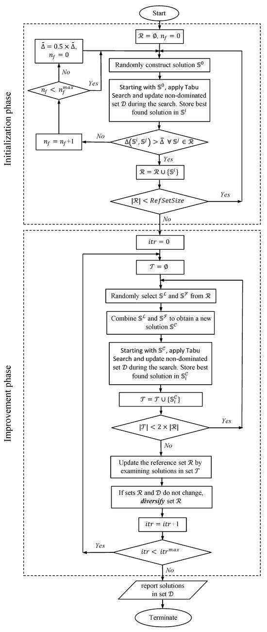
Figure 1.
Flow chart of the proposed multi-objective scatter-search metaheuristic.
In the improvement phase, a total of iterations are conducted. In each iteration, a set of trial solutions, denoted as , is constructed. This is done by randomly selecting two solutions from the reference set and then generating a new solution by combining some of their features, as described in Section 3.4. The combined solution is then improved via TS and used to update the non-dominated set . Within the steps of TS either during the construction or the improvement phase, an incumbent solution is compared with all found non-dominated solutions that are included in a set denoted as . If a non-dominated solution is found, it will be added to that set.
The newly generated solutions in set are then used to update the reference set . The size of set is limited to twice the size of the set , which in turn should not exceed the specified . The main idea behind this updating mechanism is to maintain a set of diverse and high-quality solutions in the set , which are used in generating new trial solutions. For the set of non-dominated solutions, no size restriction is imposed. If the generated solutions in set do not change the solutions in both sets, and , a diversification procedure is applied, as explained in Section 3.6. The following subsections explain the algorithmic details of the proposed MOSS metaheuristic’s main components.
3.2. Solution Representation and Construction
The operations-based (OB) representation scheme is commonly used in the applications of metaheuristic approaches to scheduling problems [4,26,31,45]. It appears in the form of a permutation that represents the sequence by which operations will be scheduled according to an interpretation algorithm, which generally chooses the earliest start times for the operations based on the given sequence. Despite its successful implementations and reported competitive results in the literature, the OB representation is many-to-one, meaning that more than one solution representation for a specific instance can result in the same generated schedule. As indicated by Abdelmaguid [4], such redundancy decreases the efficiency of the search operators of a metaheuristic. Alternatively, in this paper, we propose a representation based on vectors of permutations that correspond to the workstations visiting orders for jobs and the processing sequences on machines. It is referred to as a vectors of permutations-based (VPB) representation. The proposed representation is based on the model used in [29] for the MOSP.
To illustrate the proposed VPB chromosome structure, consider a simple instance of the studied problem for which the parameters are given in Table 1, Table 2 and Table 3. In this instance, there are five workstations, indexed according to . A machine is labeled as , where i is the assigned index of the machine in workstation w. The set of all machines is denoted as . Table 1 presents the structure of the system of the sample instance in terms of the machines that constitute each workstation and the ready times of the machines. There are six jobs to be scheduled, indexed according to . The assigned priority values for the jobs (), their release times (), and the sets of required workstations () are listed in Table 2. Lastly, the processing times, denoted as , for every job and machine , are provided in Table 3.

Table 1.
Workstations’ structure and machines’ ready times for the sample DMOSP instance.
Table 2.
Jobs’ data for the sample DMOSP instance.
Table 3.
Operations’ processing times () for the sample DMOSP instance.
The proposed VPB chromosome structure, denoted as , is constituted of two strings— and —and a vector of integer values, denoted as , representing locations in the string . The two strings are composed of sub-strings of fixed sizes, and each sub-string is composed of elements that refer to the operations to be scheduled. Figure 2 represents the chromosome structure of a solution to the considered sample instance of the studied problem. Each operation is represented by a letter that refers to its job label, as given in Table 2, followed by a number that refers to its processing workstation, as provided in Table 1. As shown in Figure 2, the two strings that constitute the chromosome structure include (the upper string), which corresponds to the orders by which jobs visit the workstations, and (the lower string), which corresponds to the operations’ processing sequences in the workstations. Meanwhile, the vector defines locations for separators that divide the workstations’ sub-strings into divisions representing the processing sequences on the machines.
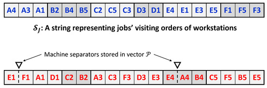
Figure 2.
Proposed solution representation for a sample solution of the presented sample DMOSP instance.
For , each sub-string corresponds to a job, and its size equals the number of operations of that job. To facilitate the visual identification of sub-strings, alternating grayscale colors are used in Figure 2. For instance, for the job labeled with the letter E, there are four elements in its sub-string. The order of the elements (operations) given in the job labeled with the letter C, for instance, indicates that job C will visit workstations in the order of 2, followed by 5, followed by 3. Accordingly, the upper string shown in Figure 2 can be directly interpreted into the vector of permutations expressed as = = = , , , , , , as in [29]. Having sub-strings with fixed sizes in the proposed chromosome structure entails that moves or exchanges of the elements as part of the search procedure of a metaheuristic will be conducted only within a sub-string; meanwhile, inter sub-string moves or exchanges are not allowed.
In , fixed-size sub-strings are defined to represent the processing sequences of operations on the machines that belong to workstations. Each sub-string corresponds to a workstation. Since a workstation may contain more than one machine, these sub-strings are divided by what is referred to as machine separators, which are defined in the vector . If workstation contains the set of machines, there will be machine separators in its sub-string. The processing sequences of the operations on the machines in set are defined using the divisions of the sub-string of workstation w. For instance, in Figure 2, the first division of the sub-string of workstation 4 contains the operation , which will be processed on the first machine, . Meanwhile, the second division contains operation , followed by operation , which will both be processed on machine in that order. The processing sequences provided in Figure 2 for the sample DMOSP instance can be easily interpreted with the vector of vectors of permutations expressed as = = , where = = , = = , = = , = = , and = = , as in [29]. Similar to the upper string, moves or exchanges as part of the search procedures of a metaheuristic must be conducted only on elements within a sub-string, and inter sub-string moves are not allowed. In addition, moves on the machine separators in the form of changing positions also need to be considered. Such moves allow for changing the sets of assigned operations for the machines in a workstation.
The decoding procedure of the proposed solution-representation scheme is based on assigning the earliest start time for each operation based on the given permutations by both strings. The pseudo-code in Algorithm 1 outlines its main steps.
| Algorithm 1 Chromosome decoder for the proposed solution-representation scheme. |
|
Algorithm 1 starts by converting the given VPB chromosome into a solution pair, , as demonstrated earlier. Then, three sets of variables are initialized. For every machine, m, the variable refers to the time at which machine m is ready to process its next operation. For every job, j, the variable refers to the time at which the job can start its next operation, while the variable refers to the job’s next operation to be scheduled, based on its given order of visiting the workstations. Then, the main loop of the algorithm constructs the schedule by iteratively scanning the next operation to be scheduled based on the processing order for each machine. If the next operation to be scheduled for job is found to be the same as the next operation to be scheduled for machine m, that operation is added to the schedule after its start and completion times are determined, and the values of its corresponding machine’s and job’s and are updated. The loop continues until all operations are scheduled. The condition of infeasibility is identified, and no schedule is returned if the search loop is terminated with remaining unscheduled operations.
Figure 3 shows the Gantt chart of the schedule generated for the solution representation shown in Figure 2 when Algorithm 1 is applied. Note that a feasible schedule generated via Algorithm 1 is semi-active, meaning that the start time of an operation cannot be set earlier without changing the processing order within its assigned machine and/or changing its job’s visiting order to its required workstations [46]. The set of semi-active schedules includes optimal solutions for many objective functions, including the ones considered in this paper. In addition, the following proposition states an important property for the relationship between the input chromosomes of Algorithm 1 and the generated schedules.
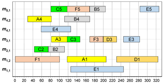
Figure 3.
Gantt chart for the generated schedule based on the solution representation shown in Figure 2 for the presented sample DMOSP instance.
Proposition 1.
For any instance of the DMOSP, a schedule generated via Algorithm 1 has one and only one input VPB chromosome.
Proof.
The proof follows from the observation that a given chromosome is interpreted to one and only one solution pair, since, as demonstrated in Figure 2, the divisions of directly correspond to the order by which jobs visit workstations, which results in one and only one , and the divisions of , as defined according to the set of positions , directly represent the processing sequences of operations on machines, which results in one and only one . Therefore, any change in , or will result in a solution pair, ≠. Let schedules and be generated via Algorithm 1 from solution pairs and , respectively, where ≠. Since Algorithm 1 is a semi-active schedule generator that schedules operations in their orders provided in a solution pair using the earliest start time for each operation, as stated in step 16, and by definition, any operation in a semi-active schedule cannot start earlier without changing the sequence to process the operations [46], . Therefore, a schedule generated via Algorithm 1 cannot have more than one input VPB chromosome. □
The property stated in Proposition 1 represents an advantage of the proposed VPB chromosome structure compared to the OB one in terms of eliminating redundancy from the chromosome domain to the solution space. Theoretically, this can help enhance the search efficiency by avoiding search moves that change the chromosome but do not change the solution. However, some guidance is needed for the search moves of the VPB representation to avoid generating chromosomes that result in infeasible solutions.
To construct solutions to be used within the proposed MOSS, the construction heuristic developed in [4] is used as is. That heuristic is based on applying different rules for selecting machines and selecting jobs to be scheduled at each iteration. Such scheduling rules tend to either improve the makespan or improve the MWFT. In addition, a random selection rule is used to allow some variability in the generated initial population. The encoding of a generated solution to its corresponding VPB chromosome is straightforward since the processing orders of operations of each job and on each machine and the jobs’ visiting order to their required workstations are clearly defined in every schedule.
3.3. Measuring Dissimilarity between Two Solutions
An essential characteristic of the scatter search metaheuristic is maintaining diversity among the solutions in the reference set along with their quality throughout both the initialization and the improvement phases. Accordingly, before a solution to set is added, its dissimilarity with existing solutions in this set is checked. This is done here by measuring the degree of dissimilarity, which is defined for any two solutions and using a distance function denoted as , which is provided in Abdelmaguid [29]. A solution can be added only when its evaluated distances with all existing solutions in set exceed a predefined limit.
The distance function is based on comparing the vectors of permutations of the two solutions, and , and counting the minimum number of moves that are needed to convert one solution to another. To illustrate how the distance function is evaluated, consider the two sample solutions shown in Figure 4 for the Bi-DMOSP instance described in Section 3.2. Determining the minimum number of moves required to convert the two strings of the second solution’s chromosome involves the determination of the common sub-strings in both chromosomes and then choosing the moves that will result in the minimal number of common sub-strings in the resulting strings. Details are provided in [29] for a computationally efficient algorithm that can be used for that task. Figure 5 illustrates the minimal moves that are required to convert the chromosome of the second solution into the first one’s. The first move (labeled with the circled number 1 in Figure 5) corresponds to exchanging the positions of operations D1 and D3 in the jobs’ string. Meanwhile, the move labeled with the number 3 corresponds to moving operation F1 after the position of the machine separator while shifting operation E1 backward in the workstations’ string. Such a move changes the sequence of processing for the operations of the machines of the workstation, and it changes the machine assignment for operation F1. Other moves are conducted similarly. As a result of the illustrated minimal moves, the distance between both solutions equals 5 in this case.
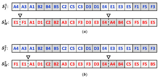
Figure 4.
Chromosomes of two sample solutions to the sample DMOSP instance presented in Section 3.2: (a) first solution and (b) second solution.
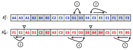
This distance function’s advantage is that it does not depend on the objective functions’ values, enabling the search procedures to explore diverse areas in the search space. To explain, consider the two sample solutions presented in Figure 4. The objective functions’ values for the first solution, , are and , and for the second solution, , they are and . Accordingly, the differences between the objective functions’ values for both solutions are not a small quantity compared to the value of . Therefore, if the distance based on the differences between the objective functions’ values is utilized, both solutions would have been added to the reference set. Nevertheless, in this case, one of the solutions would easily reach the same structure as the other one in a few neighborhood search moves. Therefore, using the value of will ensure true diversity as related to the neighborhood search moves that are utilized in the local search procedure based on tabu search.
3.4. Solution Recombination
Solution recombination is an essential operator in the search procedures of modern metaheuristics. It combines some features from parent solutions to generate a new child solution. This operator helps explore more regions in the search space between or even beyond the parent solutions. This operator appears in evolutionary metaheuristics under the name of a crossover operator [47]. In swarm-intelligence metaheuristics, the mechanism of solution recombination is conducted via position-update functions [48]. Path relinking is another form of solution-recombination operators [39].
In the current implementation of the scatter-search metaheuristic, the solution-recombination operator works as follows. First, two different parent solutions are selected randomly from the reference set, where all solutions have equal probabilities of being selected. One selected parent is labeled the leader (), and the other is labeled the follower (). These labels are used to identify the order by which genes will be inherited through the child solution ().
Figure 6 demonstrates the gene-inheriting mechanism using solutions for the sample instance presented in Section 3.2. In this mechanism, genes are inherited for each sub-string independently for both strings constituting each chromosome. For each sub-string, a number, , is randomly generated from a uniform distribution. If is greater than a predefined recombination threshold value, denoted as , the genes from the leader parent’s sub-string will be copied as-is to the child solution.
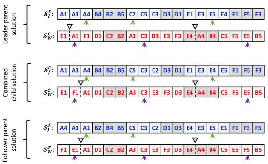
Figure 6.
Solution-recombination process.
When , genes in the child solution’s sub-string are inherited from both parents’ sub-strings as follows. First, an integer number, , is randomly generated from a discrete uniform distribution, where ℓ is the length (number of genes) of the sub-string. Figure 6 represents the randomly generated positions using a small arrow underneath the sub-strings. Then, genes from the leader solution’s sub-string are copied to the child solution’s sub-string, starting from the first gene up to the gene in location . Afterward, starting from location , the remaining genes are inherited from the follower parent using the same sequence they appear in that parent. Positions of the machine separators are inherited as-is from the parent having the larger number of inherited genes in the corresponding workstation’s sub-string, where tie-breaking is done randomly.
Since the resultant child solution can be infeasible, the recombination operator is applied a maximum of five times on the same selected parent solutions until a feasible child solution is generated. If no feasible solution is obtained after these five iterations, either the leader or the follower solution is copied to the child solution. In this case, both parents have equal copying probabilities.
3.5. A Novel Bi-Objective Tabu Search
Local improvements to solutions generated during the initialization and the improvement phases are conducted using a proposed novel bi-objective tabu search (Bi-TS) approach. This Bi-TS utilizes the two neighborhood search functions developed by Abdelmaguid [29] to improve the makespan, denoted as and . To improve the , two similar neighborhood search functions, denoted as and , are introduced here.
The neighborhood search function implements moves of operations within permutations. It performs moves on critical operations that, by definition, cannot be moved from their current positions in the permutations without affecting the current makespan [46]. Accordingly, a critical path is defined as a sequence of consecutive critical operations from start to finish. First, selects an operation belonging to the critical path, and then it investigates possible moves within the processing sequence of the job to which the selected operation belongs. The feasibility of a move and the quality of the resultant solution are derived by employing simple mathematical relationships. These relationships reduce the required computational time by avoiding the detailed evaluations of the operations’ exact start and finish times. Similarly, the neighborhood search function implements moves of critical operations within and between permutations for the machines belonging to the same workstation.
The new functions and follow the same structure of operation removal-reinsertion mechanism, as in and , respectively. This similarity allows for a unified tabu structure and tabu list for all neighborhood search moves. In and , the feasibility conditions proven by Abdelmaguid [29] for moves conducted in and are employed. Unlike and , they are applied to critical and non-critical operations. The objective values as a result of applying and are calculated by modifying the solution’s network representation, which was provided in Abdelmaguid [29]. Since this is a time-consuming process, non-critical operations that belong to the first half of a job or machine sequence are excluded from the search. This exclusion is decided after it is noticed that the value of generally does not improve by moving operations scheduled early in a given solution.
The search structure of the developed Bi-TS approach is demonstrated via the pseudo-code in Algorithm 2. It starts in steps 4 to 7 by initializing the search and iteration variables.
| Algorithm 2 Bi-objective Tabu search for the Bi-DMOSP |
|
Within the main loop, the algorithm keeps a record of the number of times each objective value is improved as a result of applying the neighborhood search functions. This is done by updating two variables, and , for recording improvements in the makespan and the MWFT objective values, respectively. These two variables are used to probabilistically determine which set of neighborhood search functions will be applied in each iteration: either or . This is done in step 10 by calling the function, which is a Boolean function that returns if a randomly generated number within the range from 0 to 1 is found to be less than the passed value p and returns otherwise. Accordingly, the ordered list is used to store the best non-tabu neighborhood moves based on the current solution . The maximum number of neighborhood moves that can be stored in the list is denoted , which is one of the control parameters of the developed Bi-TS.
From the list, either the first (best) neighborhood move or a random one is selected. Random move selection is permitted to allow for a more diversified search whenever the repeated selection of the best moves does not improve the dominance of the incumbent solution for iterations. If a random selection of moves is decided, it is repeated for at least consecutive iterations of the Bi-TS until an improvement occurs. Accordingly, this diversification mechanism is controlled via the two parameters and .
The tabu list is updated in step 18 by adding the inverse of the selected move, which is the move that will bring the solution back to its original structure before applying the selected move. If the inverse move is already included in the tabu list, the best move itself is added instead, as shown in step 19. The tabu list has a fixed size, denoted as , which cannot be exceeded. If the tabu list has moves included, the oldest move is removed.
The dominance of the incumbent solution is checked starting at step 20, when the function is applied to the difference between the objective values of the best found and the incumbent solutions. The function returns −1, 0, or +1, depending on the sign of the passed argument. If the incumbent solution is found to dominate the best found solution, a replacement is made, as shown in step 22. In such a case, the global non-dominated set of solutions, , is checked for an update. Otherwise, in step 23, if the incumbent and best found solutions do not dominate each other, set is checked for an update via an investigation of the dominance of the incumbent solution with all the solutions therein. If the incumbent solution is added to set , it will replace the current best found solution.
3.6. Updating and Diversifying Solutions in the Reference Set
During the improvement phase of the developed MOSS, the set is used to update the reference set such that does not exceed the specified fixed value of the parameter . This is done by first removing all solutions from set and adding them to set . Then, an ordered list, , is generated based on solutions in in which solutions are ordered based on their dominance relations. That is, if dominates , will be ordered first, and vice versa. If the two solutions do not dominate each other, their order will be arbitrary.
In the given solutions’ order in , solutions are iteratively added to set until its size reaches . To maintain the diversity of the solutions in set , before a solution is added, its distance from every already added solution is evaluated as described in Section 3.3. This distance must exceed the predefined distance threshold value (). Otherwise, the solution will not be added. After all solutions in are examined, if the size of the resultant set is found to be less than , additional solutions will be generated and added to it using the same procedure described in the construction process, as in Section 3.2.
The developed reference set-updating procedure aims to maintain both solution quality and diversity throughout iterations. Furthermore, to avoid long-term entrapment in local optimal solutions, a diversification strategy is annexed to the reference set-updating process. In this strategy, the percentage changes in the summations of the values of the makespan and the MWFT for all solutions in set are evaluated before and after every improvement cycle. If these percentage changes are found to be less than 2%, and the set of non-dominated solutions (set ) has not been changed by adding new solutions during the improvement cycle, the solutions in the reference set will be diversified. The diversification is achieved by replacing one-quarter of the solutions with newly constructed ones using the construction procedure described in Section 3.2. New randomly constructed solutions are improved using tabu search, as usual. In addition, at most one-quarter of the solutions in the reference set are replaced with solutions selected arbitrarily from the non-dominated set .
4. Performance Metrics
Many metrics have been proposed in the literature to assess the performance of multi-objective optimization algorithms [49]. The simplest of them is the number of non-dominated solutions that a metaheuristic generates (). This metric is an indication of the capability of a metaheuristic to generate alternative non-dominated solutions. However, it does not provide any clue about their quality. Whenever the set of optimal Pareto front solutions () is known for an instance, the gravitational distance () and the inverted gravitational distance () can be used to assess the quality of the generated non-dominated solutions via a heuristic () with respect to the solutions in set . These metrics are evaluated using Equations (1) and (2) below.
where,
Both metrics are suitable for the studied DMOSP since it is a discrete optimization problem characterized by a small number of non-dominated solutions for the considered objectives [3,4]. Small values for both metrics are favorable, and zero values for both indicate that = . The main difference between and is that the former indicates how successful the heuristic is in reaching solutions close to a subset of the solutions in set . However, it fails to indicate whether or not a heuristic can find solutions with proximity to all solutions in set (i.e., covering all optimal Pareto front solutions). Meanwhile, the latter metric measures the closeness of solutions in set to their nearest ones in set . This inherently checks for the ability of a heuristic to cover all solutions in set . However, unlike , it fails to account for the negative effect of inferior non-dominated solutions in set that can be quite far from the optimal Pareto front. This paper proposes a combined metric, the total gravitational distance (), calculated as . The attempts to combine the benefits of and metrics and subdue their shortcomings. As a result, small values for indicate that the heuristic results in solutions close to the Pareto front with good coverage.
For large-sized instances with unknown Pareto front solutions, the performance of a multi-objective optimization algorithm can be compared to benchmark algorithms using hypervolume (HV), which was introduced by [50]. The reference point used here to calculate the hypervolume is arbitrarily selected as = and = , where and are the lower bounds for the makespan and the MWFT of a DMOSP instance, respectively. The evaluation formulas for the lower bounds are provided in [4]. In this paper, the percentage hypervolume measure () introduced by [4] is used to compare the performance of the developed MOSS with the previously developed NSGA-II approach. The is a relative measure in which the value of is divided by the area of the rectangle defined according to the two vertexes and , as expressed in Equation (3).
When comparing two multi-objective optimization algorithms, a higher value signifies better performance. Whenever set is known for an instance, the percentage hypervolume deviation, defined in Equation (4), can be used as an alternative assessment metric. A low value indicates good performance, and whenever , it means .
5. Computational Experiments, Results, and Discussion
The developed MOSS was programmed using the C++ programming language. Like the previously developed NSGA-II approach in Abdelmaguid [4], the Embarcadero 32-bit C++ compiler, version 6.2, was used to generate the executable code. Computational experiments were conducted using a desktop computer with Intel Core i3-7100 dual-core processor running at a clock speed of 3.90 GHz, with a physical memory of 8 GB, that operated on Windows 10. Firstly, fine-tuning computational experiments were used to guide the selection of the parameters of the developed MOSS. Secondly, computational experiments were conducted to assess its performance by comparing its generated non-dominated solutions with exact Pareto front solutions obtained for small-sized instances and solutions obtained using the previously developed NSGA-II approach for small- and large-sized instances.
5.1. Tuning MOSS Parameters
Before conducting performance assessment experiments for the developed MOSS, tuning experiments were performed to guide the selection of the best values of its parameters. This was done here using selected small-sized test instances for which the optimal Pareto front solutions were known. These instances were selected from the testbed provided in Abdelmaguid [3], for which the -constraint method was used in finding the optimal Pareto front solutions. Six small instances from the thirty instances provided in Abdelmaguid [3] were selected for the tuning experiments. They were selected such that there was diversity in their values, which equal 2, 4, 8, 11, 14, and 17. This diversity was the result of variation in the structures of these six instances that was necessary to avoid biased results. The MOSS parameters included in the tuning experiments and their selected levels are listed in Table 4.
Table 4.
Factors considered in the parameter-tuning experiments and their levels.
Another MOSS parameter is , which defines the distance limit that must be exceeded by a solution to be added to the reference set. This parameter is problem-specific and determined using the formula provided in Abdelmaguid [29], as provided in Equation (5). The value of the constant was set to 3 for small-sized instances and 5 for large-size ones. A small instance was arbitrarily identified with a total number of operations less than 50.
Three independent runs were conducted for each treatment combination. Therefore, a total of = 39,366 independent runs were conducted in a random order. For each run, = 100, and there was no time limit. For each run, the values of , and the computational time () were recorded. Since the number of iterations was fixed for all runs, the reported average total computational time for a treatment combination allowed for estimating the average computational time requirement at the selected levels of the MOSS parameters.
Figure 7a shows the main effect plots for . It was noticed that the main effects plots for demonstrated the same behavior; therefore, they were not included here. Meanwhile, Figure 7b shows the main effects plots for the computational time. Based on these plots and the analysis of variance (ANOVA) results at 95% confidence level, the levels of the variables that will result in the lowest average and , such that they do not affect the average computational time, were selected as follows: , , , , and . There is an apparent tradeoff between the solution quality and the computational time requirement for the remaining two parameters, and . This means that, if there is a computational time limit, the selected levels of both parameters, which resulted in low-quality solutions yet low computational times in these tuning experiments, can result in good-quality solutions because they allow the algorithm to conduct a larger number of iterations. Therefore, additional tuning experiments were conducted to help select appropriate levels for these two parameters.
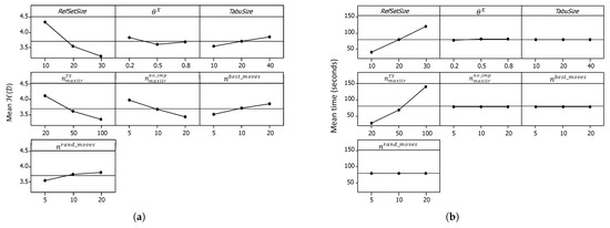
Figure 7.
Main effect plots from the first MOSS-tuning experiments. (a) Main effect plots for . (b) Main effect plots for the computational time.
In the additional tuning experiments, there was no limit on the number of iterations, and the computational time was restricted to 120 s. The values of and were recorded at the end of the initialization phase and every 30 s afterward. The selected levels in the additional tuning experiments focused on the values of 15, 20, 25, 30, 35, and 40 for and the values of 40, 50, 80, 100, 150, and 200 for . Lower values for both parameters were excluded, as their results in the former tuning experiments showed deficient performance. Using the same set of small-sized instances with six values for , and conducting 30 independent runs for each treatment combination, revealed a total of = 6480 independent runs that were conducted in random order.
Figure 8 summarizes the average computational performance for the second MOSS-tuning experiments throughout the improvement phase. It is evident that the quality of the solutions at the end of the initialization phase increased with the increase in both and . However, this characteristic was quickly reversed, as the developed MOSS, after 30 s, produced better results with low values for both parameters. This continued as time proceeded. For the average , the effect of is evident in Figure 8b, while the effect of is apparently lower, as shown in Figure 8a. The same behavior can be noticed for the average , as shown in Figure 8c,d. These results suggest that low values for at 15 or 20 and low values of at 40 or 50 can produce good-quality solutions in short computational times.
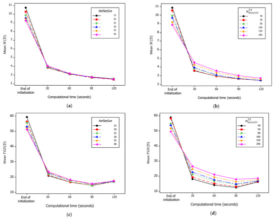
Figure 8.
Progress of average performance over computational time in the second MOSS-tuning experiments. (a) Mean at different values. (b) Mean at different values. (c) Mean at different values. (d) Mean at different values.
In addition to the conclusions about the preferred levels of the MOSS parameters, there was an important phenomenon involving the measure that is worth mentioning here. Figure 8c,d show that, unlike , which is monotone non-increasing with respect to the computational time, the value of can increase despite the improvement in the solutions in set . This increase is apparent in Figure 8c,d after 90 s of computational time. The reason behind this phenomenon is that the evaluation of the performance measures is based only on the found set of non-dominated solutions at any given time. If better non-dominated solutions are found, other solutions that were non-dominated in a previous iteration and become now dominated are removed from set , and therefore, they are no longer used in evaluating the performance measures. When the is evaluated, there could be a non-dominated solution that is close to one of the optimal Pareto front solutions in a previous iteration, which is then dominated by another solution that is far from that Pareto optimal solution. This phenomenon indicates that the gravitational distance measures do not have the consistency of the hypervolume-based measures.
5.2. Results for Small-Sized Instances
In this section, computational experiments on small-sized instances are conducted to compare the performance of the developed MOSS with the best metaheuristic found in the literature for the DMOSP, which is based on NSGA-II [4], along with the comparison with the optimal Pareto front solutions obtained using the -constraint method [3]. These experiments utilized a set of 30 small-sized instances with that ranged from 1 to 23. Based on the results of the tuning experiments in the previous section, the levels of the MOSS parameters were chosen as , , , , , , and . Both NSGA-II and MOSS were run with a computational time limit of 60 s.
For each DMOSP small instance, the average performance metrics, namely the mode of (), its average (), the average total gravitational distance (), and the average percentage hypervolume deviation (), were calculated based on the thirty independent runs conducted using each metaheuristic. Table 5 lists these values. It is important to note that there are minor differences in the NSGA-II results reported here compared to Abdelmaguid [4] since the computational time limit here was 60 s instead of 30 s. Boldface is used in Table 5 to highlight the best value for each metric when both metaheuristics’ results are compared.
Table 5.
Summary of computational results statistics for small benchmark instances of both NSGA-II and MOSS.
When comparing the two measures of the resultant number of non-dominated solutions (), namely the mode and the average , as reported in Table 5, it is evident that the developed MOSS is capable of producing a larger number of non-dominated solutions in 18 instances, versus only 3 for the NSGA-II based on the mode. Meanwhile, for the average, MOSS resulted in better values in 24 instances versus 5 for NSGA-II. Therefore, it can be concluded that the developed MOSS has better search capability that enables it to find more non-dominated solutions compared to NSGA-II.
As illustrated in Table 5, the developed MOSS resulted in better in 25 instances. Similarly, for , MOSS resulted in better values in 25 instances. For both metrics combined, MOSS resulted in better values in 23 instances versus only 3 for NSGA-II. As an overall average performance for the 30 instances, the average TGD of MOSS was 12.84, compared to 18.90 for NSGA-II, and the average percentage hypervolume deviation of MOSS was 1.83, as opposed to 2.74 for NSGA-II. To statistically compare these results, a paired t-test was conducted on and . The paired t-test was suitable for this comparison since the experiments were conducted on the same group of MOSS instances, and the calculated averages were approximately normally distributed due to the central limit theorem. Figure 9 shows the box-and-whisker plots for the mean differences of both metrics, along with the confidence interval at a 95% confidence level of the null hypothesis (). Here, is stated as the difference of the means equaling zero.
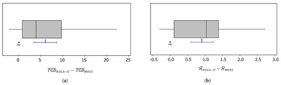
Figure 9.
Box-and-whisker plots and confidence intervals for the average difference in and , based on the results of a paired t-test for the computational experiments on small-sized instances at a 95% confidence level. (a) Results for total gravitational distances. (b) Results for the percentage hypervolume deviations.
Statistical results show that the mean value of was 6.06 with a 95% confidence interval of [3.50,8.62]. Meanwhile, the mean value of was 0.908 with a 95% confidence interval of [0.593, 1.223]. These means (labeled as ) and confidence intervals are presented in Figure 9 using blue-colored lines. Based on these results, it can be concluded that, at a 95% confidence level, the metrics of the developed MOSS are significantly better than those of NSGA-II.
To illustrate detailed results for the small-sized test instances, Figure 10 shows the generated set of non-dominated solutions by both metaheuristics for six selected instances, along with their optimal Pareto front solutions. The Figure 10a–f are ordered in ascending order for the number of optimal Pareto front solutions of the instance, as reported in Table 5. Even though these results were recorded for only one run of each metaheuristic with a computational time limit of 120 s, they reflect the true performance of both metaheuristics that complies with the reported mean results in Table 5 and Figure 9. Based on Figure 10, it is evident that the developed MOSS can generate efficient, non-dominated solutions that are very close to the optimal Pareto front with a better spread and better quality compared to the previously developed NSGA-II.
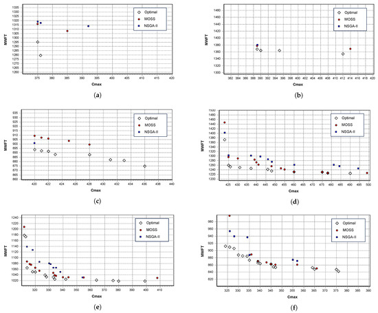
Figure 10.
Pareto fronts and generated non-dominated solutions of both NSGA-II and MOSS for selected small-sized instances. (a) DMOSP-S-7. (b) DMOSP-S-6. (c) DMOSP-S-24. (d) DMOSP-S-17. (e) DMOSP-S-4. (f) DMOSP-S-15.
5.3. Results for Large-Sized Instances
The purpose of the computational experiments conducted using large-sized instances was to compare the performance of both MOSS and NSGA-II at different levels of the problem parameters. The main problem parameters that define its structure include the number of workstations (), the number of jobs (), the loading level (), the percentage of late-arriving jobs (), and the percentage of busy machines (). As defined in [3], is used during the instance generation to determine whether a job requires processing in a workstation randomly. This is done by generating a uniform random number (u) between 0 and 1 and comparing it to the value of . If , the job will require processing in the workstation. During the instance-generation procedure, this process is repeated for all jobs and workstations. The value of is between 0 and 1, and the higher the value of , the more dense the schedule will be.
Since the studied DMOSP is characterized by a subset of jobs with non-zero arrival times, the parameter was used in instance generation to account for this characteristic. The value of was defined as a decimal number between 0 and 100. During the release time generation of an instance, a uniform random number, , was generated, and its value was compared to . Whenever , zero release time was assigned to that job. Otherwise, a non-zero release time was randomly generated. Similarly, a machine can be busy at the beginning of a rescheduling phase and, therefore, have a non-zero available time. This is represented using the parameter, which is used similarly as in the instance-generation process.
The chosen levels for the mentioned problem structural parameters are shown in Table 6. All values of the processing times of jobs on machines, job arrival times, and machines’ available times were randomly generated for each instance using the procedure described in [3].
Table 6.
Selected levels of the structural parameters used in generating large DMOSP instances.
Based on a consideration of five structural parameters with two levels each, a fractional factorial design was used. This experimental design was suitable for the requirements of the current comparison since more than two-factor interactions were not of concern. At each treatment combination, 10 instances were randomly generated. For each instance, there were 30 independent runs conducted using each metaheuristic. This resulted in a total of 4800 independent runs for each metaheuristic. The computational time of a run was limited to seconds. For NSGA-II runs, the best parameters determined in [4] were utilized. The algorithmic parameters used for small instances were used for the developed MOSS, except that the value of was set to 10. As reported earlier in the parameter-tuning experiments, this was not expected to reduce the quality of generated solutions, yet it reduced the computational effort needed.
For each randomly generated instance, the average of the 30 values obtained via a metaheuristic was calculated and denoted . Accordingly, the difference between the MOSS result () and the NSGA-II result () was denoted and evaluated as . The values of at all treatment combinations were used as the response in comparing the results of both metaheuristics. Clearly, positive values of indicate the better performance of MOSS over NSGA-II.
For , Figure 11 shows the main effects plots, while Figure 12 shows the interaction plots. As shown in Figure 11, the mean value of became slightly below 0 at higher and values. Meanwhile, the effect of the other three factors remained in the positive domain despite being significant at 95% confidence, based on the analysis of variance (ANOVA) results. Meanwhile, the interaction plots of Figure 12 show that higher values of combined with higher values of , as well as higher values of combined with higher values of , resulted in larger negative values for the response. Accordingly, it can be concluded that the developed MOSS demonstrated better performance compared to NSGA-II for cases with low and intermediate density, while this situation was reversed for more dense cases.
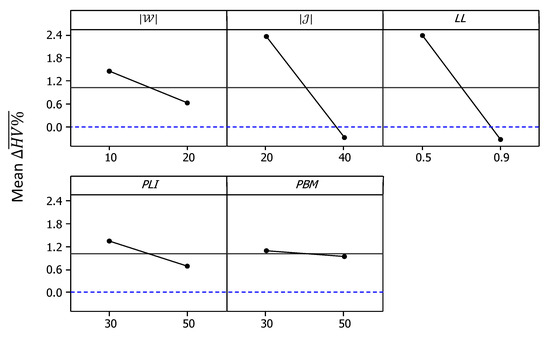
Figure 11.
Main effect plots for .
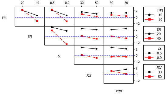
Figure 12.
Interaction plots for .
6. Conclusions and Future Research
In this paper, a novel metaheuristic approach based on scatter search was developed to provide efficient, non-dominated solutions to a bi-objective, dynamic, multi-processor open-shop scheduling problem (Bi-DMOSP). This problem is frequently encountered in maintenance and healthcare diagnostic applications, and therefore, providing efficient solutions is particularly important to effectively manage these systems. The two objectives considered in this paper were the minimization of the makespan and the minimization of the mean weighted flow time (MWFT). The former objective targets maximizing the utilization of the available machines, while the latter aims to improve customer satisfaction.
Since the studied problem is known to be NP-hard for both objectives, their simultaneous consideration represents a challenge in designing efficient algorithmic approaches. This paper adopted a multi-objective scatter-search (MOSS) approach combined with an efficient novel bi-objective tabu search for local improvements. It is intended to reduce the computational burden caused by the large size of the solution set and the redundant local search moves found in a formerly developed metaheuristic based on NSGA-II. The developed metaheuristic in this paper utilizes a small set of reference solutions to generate a new set of test solutions in every iteration, combined with an efficient bi-objective tabu search that targets improving both objectives. With an efficient updating mechanism for the reference and non-dominated solutions throughout iterations, the developed metaheuristic can effectively achieve the stated quest of finding efficient non-dominated solutions.
Computational experiments were conducted on randomly generated small and large instances of the studied Bi-DMOSP. Thirty small-sized benchmark instances were used to fine-tune the metaheuristic parameters and compare their performance against the formerly developed NSGA-II and an exact algorithm based on the -constraint method. Three performance metrics were used in the comparisons: the number of generated non-dominated solutions, the total gravitational distance, and the percentage hypervolume deviation. The last two performance metrics were developed in this paper to represent deviations from the known optimal Pareto front, obtained earlier using the -constraint method. Computational results revealed the superiority of the developed MOSS compared to NSGA-II, resulting in better metrics in 23 instances versus only three instances for NSGA-II. Meanwhile, at a 95% confidence level, the developed MOSS’s overall average performance was significantly better. Furthermore, the average percentage hypervolume deviation of the developed MOSS was found to be only 1.83% versus 2.74% for NSGA-II, which reflects its capability of generating non-dominated solutions that are very close to the optimal Pareto front and its superiority over NSGA-II.
The large-sized instances are randomly generated at different levels of selected problem parameters representing its structure. These parameters include the number of workstations, the number of jobs, the loading level (percentage of workstations needed for a job), and two parameters representing the job release and machine-ready times. Computational results reveal that the difference between the developed MOSS and NSGA-II in terms of their percentage hypervolumes is mainly affected by the first three parameters. It was found that the developed MOSS can produce competitive results in cases of low density, which are measured by the loading level, combined with the number of jobs. Meanwhile, this was reversed in the cases with large densities.
The studied Bi-DMOSP is, undoubtedly, an important problem in maintenance and healthcare applications. Providing efficient Pareto front solutions to this problem is of utmost importance for efficiently managing such systems. The results presented in this paper provide some insights that can guide managerial decisions regarding the solution algorithm to be implemented in a specific situation. If the problem size is small (five jobs and five workstations), obtaining an optimal Pareto front can possibly be done in a reasonable computational time using the exact algorithm presented in [3]. For larger cases, the developed hybrid metaheuristic approach presented in this paper is a competitive candidate that can be used to generate efficient non-dominated solutions that are very close to the unknown optimal Pareto front for medium and large cases with low density. An alternative NSGA-II approach, as presented in [4], can provide efficient solutions for large cases with high density levels.
Since the studied Bi-DMOSP is NP-hard, its future algorithmic development will remain open for more efficient approaches. Some algorithmic techniques developed in this paper, especially the local search mechanism, can be further refined and extended by incorporating more efficient neighborhood search functions. More specifically, the suggested neighborhood search functions used for improving the MWFT are at a different speed than those used for improving the makespan, since they require reconstructing the whole network representation of the problem to evaluate the objective value. Quicker methods for estimating the effect of the neighborhood moves on the MWFT can significantly reduce the computational time. This could improve the results of the developed MOSS for large-sized dense cases. Another direction for future algorithmic development is the consideration of an automated parameter-tuning approach, such as irace [51], which attempts to optimize the algorithm parameters as an integrated part of its execution. They can be compared with the static parameter-tuning approach followed in this paper.
Other future research extensions can include the customization of the developed MOSS approach for more general cases of the studied problem, as well as similar multiprocessor shop-scheduling problems. For instance, the developed MOSS approach can be applied to multi-processor-flow shop-scheduling and flexible-job shop-scheduling problems. The structure of the studied Bi-DMOSP can be extended to include the cases of sequence-dependent setup times, planned maintenance activities, and the scheduling of material handling equipment.
Funding
This research received no external funding.
Data Availability Statement
The dataset is available upon request from the author.
Conflicts of Interest
The author declares no conflicts of interest.
References
- Werner, F. Special Issue “Scheduling: Algorithms and Applications”. Algorithms 2023, 16, 268. [Google Scholar] [CrossRef]
- Uhlmann, I.R.; Frazzon, E.M. Production rescheduling review: Opportunities for industrial integration and practical applications. J. Manuf. Syst. 2018, 49, 186–193. [Google Scholar] [CrossRef]
- Abdelmaguid, T.F. Bi-Objective Dynamic Multiprocessor Open Shop Scheduling: An Exact Algorithm. Algorithms 2020, 13, 74. [Google Scholar] [CrossRef]
- Abdelmaguid, T.F. Bi-objective dynamic multiprocessor open shop scheduling for maintenance and healthcare diagnostics. Expert Syst. Appl. 2021, 186, 115777. [Google Scholar] [CrossRef]
- Hwang, C.L.; Masud, A.S.M. Multiple Objective Decision Making—Methods and Applications: A State-of-the-Art Survey; Springer: Berlin/Heidelberg, Germany, 1979; Volume 164. [Google Scholar] [CrossRef]
- Gonzalez, T.; Sahni, S. Open Shop Scheduling to Minimize Finish Time. J. Assoc. Comput. Mach. 1976, 23, 665–679. [Google Scholar]
- Achugbue, J.O.; Chin, F.Y. Scheduling the open shop to minimize mean flow time. SIAM J. Comput. 1982, 11, 709–720. [Google Scholar] [CrossRef]
- Wang, Y.T.H.; Chou, F.D. A Bi-criterion Simulated Annealing Method to Solve Four-Stage Multiprocessor Open Shops with Dynamic Job Release Time. In Proceedings of the 2017 International Conference on Computing Intelligence and Information System (CIIS), Nanjing, China, 21–23 April 2017; pp. 13–17. [Google Scholar] [CrossRef]
- Deb, K.; Pratap, A.; Agarwal, S.; Meyarivan, T. A fast and elitist multiobjective genetic algorithm: NSGA-II. IEEE Trans. Evol. Comput. 2002, 6, 182–197. [Google Scholar] [CrossRef]
- Mirjalili, S.; Saremi, S.; Mirjalili, S.M.; dos S. Coelho, L. Multi-objective grey wolf optimizer: A novel algorithm for multi-criterion optimization. Expert Syst. Appl. 2016, 47, 106–119. [Google Scholar] [CrossRef]
- Abreu, L.R.; Prata, B.A.; Framinan, J.M.; Nagano, M.S. New efficient heuristics for scheduling open shops with makespan minimization. Comput. Oper. Res. 2022, 142, 105744. [Google Scholar] [CrossRef]
- Ahmadian, M.M.; Khatami, M.; Salehipour, A.; Cheng, T.C. Four decades of research on the open-shop scheduling problem to minimize the makespan. Eur. J. Oper. Res. 2021, 295, 399–426. [Google Scholar] [CrossRef]
- Bräsel, H.; Herms, A.; Mörig, M.; Tautenhahn, T.; Tusch, J.; Werner, F. Heuristic constructive algorithms for open shop scheduling to minimize mean flow time. Eur. J. Oper. Res. 2008, 189, 856–870. [Google Scholar] [CrossRef]
- Tang, L.; Bai, D. A new heuristic for open shop total completion time problem. Appl. Math. Model. 2010, 34, 735–743. [Google Scholar] [CrossRef]
- Andresen, M.; Bräsel, H.; Mörig, M.; Tusch, J.; Werner, F.; Willenius, P. Simulated annealing and genetic algorithms for minimizing mean flow time in an open shop. Math. Comput. Model. 2008, 48, 1279–1293. [Google Scholar] [CrossRef]
- Bai, D.; Zhang, Z.; Zhang, Q.; Tang, M. Open shop scheduling problem to minimize total weighted completion time. Eng. Optimiz. 2017, 49, 98–112. [Google Scholar] [CrossRef]
- Sha, D.Y.; Lin, H.h.; Hsu, C.Y. A Modified Particle Swarm Optimization for Multi-objective Open Shop Scheduling. In Proceedings of the International MultiConference of Engineers and Computer Scientists 2010 (IMECS 2010), Hong Kong, China, 17–19 March 2010; Volume 3, pp. 1844–1848. [Google Scholar]
- Tavakkoli-Moghaddam, R.; Panahi, H.; Heydar, M. Minimization of weighted tardiness and makespan in an open shop environment by a novel hybrid multi-objective meta-heuristic method. In Proceedings of the 2008 IEEE International Conference on Industrial Engineering and Engineering Management, Singapore, 8–11 December 2008; pp. 379–383. [Google Scholar] [CrossRef]
- Panahi, H.; Tavakkoli-Moghaddam, R. Solving a multi-objective open shop scheduling problem by a novel hybrid ant colony optimization. Expert Syst. Appl. 2011, 38, 2817–2822. [Google Scholar] [CrossRef]
- Seraj, O.; Tavakkoli-Moghaddam, R.; Jolai, F. A fuzzy multi-objective tabu-search method for a new bi-objective open shop scheduling problem. In Proceedings of the 2009 International Conference on Computers Industrial Engineering, Troyes, France, 6–9 July 2009; pp. 164–169. [Google Scholar] [CrossRef]
- Naderi, B.; Mousakhani, M.; Khalili, M. Scheduling multi-objective open shop scheduling using a hybrid immune algorithm. Int. J. Adv. Manuf. Technol. 2013, 66, 895–905. [Google Scholar] [CrossRef]
- Adak, Z.; Akan, M.Ö.; Bulkan, S. Multiprocessor open shop problem: Literature review and future directions. J. Comb. Optim. 2020, 40, 547–569. [Google Scholar] [CrossRef]
- Schuurman, P.; Woeginger, G.J. Approximation algorithms for the multiprocessor open shop scheduling problem. Oper. Res. Lett. 1999, 24, 157–163. [Google Scholar]
- Jansen, K.; Sviridenko, M. Polynomial Time Approximation Schemes for the Multiprocessor Open and Flow Shop Scheduling Problem. In STACS 2000; Reichel, H., Tison, S., Eds.; Lecture Notes in Computer Science; Springer: Berlin/Heidelberg, Germany, 2000; Volume 1770, pp. 455–465. [Google Scholar] [CrossRef]
- Sevastianov, S.; Woeginger, G. Linear time approximation scheme for the multiprocessor open shop problem. Discret. Appl. Math. 2001, 114, 273–288. [Google Scholar] [CrossRef][Green Version]
- Naderi, B.; Fatemi Ghomi, S.; Aminnayeri, M.; Zandieh, M. Scheduling open shops with parallel machines to minimize total completion time. J. Comput. Appl. Math. 2011, 235, 1275–1287. [Google Scholar] [CrossRef]
- Fu, Y.; Li, H.; Huang, M.; Xiao, H. Bi-Objective Modeling and Optimization for Stochastic Two-Stage Open Shop Scheduling Problems in the Sharing Economy. IEEE Trans. Eng. Manag. 2023, 70, 3395–3409. [Google Scholar] [CrossRef]
- Fu, Y.; Zhou, M.; Guo, X.; Qi, L.; Gao, K.; Albeshri, A. Multiobjective Scheduling of Energy-Efficient Stochastic Hybrid Open Shop With Brain Storm Optimization and Simulation Evaluation. IEEE Trans. Syst. Man Cybern. Syst. 2024, 54, 4260–4272. [Google Scholar] [CrossRef]
- Abdelmaguid, T.F. Scatter Search with Path Relinking for Multiprocessor Open Shop Scheduling. Comput. Ind. Eng. 2020, 141, 106292. [Google Scholar] [CrossRef]
- Behnamian, J.; Memar Dezfooli, S.; Asgari, H. A scatter search algorithm with a novel solution representation for flexible open shop scheduling: A multi-objective optimization. J. Supercomput. 2021, 77, 13115–13138. [Google Scholar] [CrossRef]
- Matta, M.E. A genetic algorithm for the proportionate multiprocessor open shop. Comput. Oper. Res. 2009, 36, 2601–2618. [Google Scholar] [CrossRef]
- Abdelmaguid, T.F.; Shalaby, M.A.; Awwad, M.A. A tabu search approach for proportionate multiprocessor open shop scheduling. Comput. Optim. Appl. 2014, 58, 187–203. [Google Scholar] [CrossRef]
- Abdelmaguid, T.F. A Hybrid PSO-TS Approach for Proportionate Multiprocessor Open Shop Scheduling. In Proceedings of the 2014 IEEE International Conference on Industrial Engineering and Engineering Management (IEEM), Kuala Lumpur, Malaysia, 9–12 December 2014; pp. 107–111. [Google Scholar]
- Zhang, J.; Wang, L.; Xing, L. Large-scale medical examination scheduling technology based on intelligent optimization. J. Comb. Optim. 2019, 37, 385–404. [Google Scholar] [CrossRef]
- Adak, Z.; Övül, M.; Bulkan, S. An ant colony optimization approach for the proportionate multiprocessor open shop. J. Comb. Optim. 2021, 43, 785–817. [Google Scholar] [CrossRef]
- Bai, D.; Zhang, Z.H.; Zhang, Q. Flexible open shop scheduling problem to minimize makespan. Comput. Oper. Res. 2016, 67, 207–215. [Google Scholar] [CrossRef]
- Ma, X.; Fu, Y.; Gao, K.; Zhu, L.; Sadollah, A. A Multi-Objective Scheduling and Routing Problem for Home Health Care Services via Brain Storm Optimization. Complex Syst. Model. Simul. 2023, 3, 32–46. [Google Scholar] [CrossRef]
- Fu, Y.; Ma, X.; Gao, K.; Li, Z.; Dong, H. Multi-Objective Home Health Care Routing and Scheduling With Sharing Service via a Problem-Specific Knowledge-Based Artificial Bee Colony Algorithm. IEEE Trans. Intell. Transp. Syst. 2024, 25, 1706–1719. [Google Scholar] [CrossRef]
- Glover, F. A template for scatter search and path relinking. Lect. Notes Comput. Sci. 1998, 1363, 3–51. [Google Scholar] [CrossRef]
- Martí, R.; Lourenço, H.; Laguna, M. Assigning Proctors to Exams with Scatter Search. In Computing Tools for Modeling, Optimization and Simulation; Laguna, M., Velarde Gonzales, J.L., Eds.; Kluwer Academic Publishers: Dordrecht, The Netherlands, 2000; pp. 215–228. [Google Scholar]
- Nebro, A.J.; Luna, F.; Alba, E. New Ideas in Applying Scatter Search to Multiobjective Optimization. In Evolutionary Multi-Criterion Optimization; Coello Coello, C.A., Hernández Aguirre, A., Zitzler, E., Eds.; Springer: Berlin/Heidelberg, Germany, 2005; pp. 443–458. [Google Scholar] [CrossRef]
- Beausoleil, R.P. “MOSS” Multiobjective scatter search applied to non-linear multiple criteria optimization. Eur. J. Oper. Res. 2006, 169, 426–449. [Google Scholar] [CrossRef]
- Rahimi-Vahed, A.R.; Javadi, B.; Rabbani, M.; Tavakkoli-Moghaddam, R. A multi-objective scatter search for a bi-criteria no-wait flow shop scheduling problem. Eng. Optimiz. 2008, 40, 331–346. [Google Scholar] [CrossRef]
- Engin, O.; Kahraman, C.; Yilmaz, M.K. A scatter search method for multiobjective fuzzy permutation flow shop scheduling problem: A real world application. In Studies in Computational Intelligence; Springer: Berlin/Heidelberg, Germany, 2009; Volume 230, pp. 169–189. [Google Scholar] [CrossRef]
- Low, C.; Yeh, Y. Genetic algorithm-based heuristics for an open shop scheduling problem with setup, processing, and removal times separated. Robot. Cim. Int. Manuf. 2009, 25, 314–322. [Google Scholar] [CrossRef]
- Pinedo, M. Scheduling: Theory, Algorithms, and Systems, 5th ed.; Springer: Cham, Switzerland, 2016. [Google Scholar]
- Gen, M.; Cheng, R. Genetic Algorithms and Engineering Optimization; John Wiley & Sons, Inc.: Cambridge, MA, USA, 2000. [Google Scholar] [CrossRef]
- Kennedy, J.; Eberhart, R. Particle swarm optimization. In Proceedings of the ICNN’95—International Conference on Neural Networks, Perth, WA, Australia, 27 November–1 December 1995; Volume 4, pp. 1942–1948. [Google Scholar] [CrossRef]
- Li, M.; Yao, X. Quality evaluation of solution sets in multiobjective optimisation: A survey. ACM Comput. Surv. 2019, 52, 26. [Google Scholar] [CrossRef]
- Zitzler, E.; Thiele, L. Multiobjective evolutionary algorithms: A comparative case study and the strength Pareto approach. IEEE Trans. Evol. Comput. 1999, 3, 257–271. [Google Scholar] [CrossRef]
- López-Ibáñez, M.; Dubois-Lacoste, J.; Pérez Cáceres, L.; Birattari, M.; Stützle, T. The irace package: Iterated racing for automatic algorithm configuration. Oper. Res. Perspect. 2016, 3, 43–58. [Google Scholar] [CrossRef]


Disclaimer/Publisher’s Note: The statements, opinions and data contained in all publications are solely those of the individual author(s) and contributor(s) and not of MDPI and/or the editor(s). MDPI and/or the editor(s) disclaim responsibility for any injury to people or property resulting from any ideas, methods, instructions or products referred to in the content. |
© 2024 by the author. Licensee MDPI, Basel, Switzerland. This article is an open access article distributed under the terms and conditions of the Creative Commons Attribution (CC BY) license (https://creativecommons.org/licenses/by/4.0/).