Multithreading-Based Algorithm for High-Performance Tchebichef Polynomials with Higher Orders

Abstract

Tchebichef polynomials (TPs) play a crucial role in various fields of mathematics and applied sciences, including numerical analysis, image and signal processing, and computer vision. This is due to the unique properties of the TPs and their remarkable performance. Nowadays, the demand for high-quality images (2D signals) is increasing and is expected to continue growing. The processing of these signals requires the generation of accurate and fast polynomials. The existing algorithms generate the TPs sequentially, and this is considered as computationally costly for high-order and larger-sized polynomials. To this end, we present a new efficient solution to overcome the limitation of sequential algorithms. The presented algorithm uses the parallel processing paradigm to leverage the computation cost. This is performed by utilizing the multicore and multithreading features of a CPU. The implementation of multithreaded algorithms for computing TP coefficients segments the computations into sub-tasks. These sub-tasks are executed concurrently on several threads across the available cores. The performance of the multithreaded algorithm is evaluated on various TP sizes, which demonstrates a significant improvement in computation time. Furthermore, a selection for the appropriate number of threads for the proposed algorithm is introduced. The results reveal that the proposed algorithm enhances the computation performance to provide a quick, steady, and accurate computation of the TP coefficients, making it a practical solution for different applications.

1. Introduction

Orthogonal polynomials (OPs) and their moments substantially contribute to diverse domains due to their unique properties and broad applications. For example, the orthogonality of the OPs simplifies the mathematical computations, particularly in solving equations and approximation theory [1]. Moreover, OPs are essential in numerical analysis for exact integration schemes like Gaussian quadrature [2]. In statistics, OPs are vital for polynomial regression [3]. Additionally, OPs are considered crucial in quantum mechanics for solving the Schrödinger equation [4]. Furthermore, OPs are important tools in signal and image processing for their efficient signal representation, filter design, signal reconstruction, and feature extraction [5,6,7,8,9]. Examples of OPs are Krawtchouk [10], Charlier [11], Hahn [12,13], Racah [14,15], Legendre [16], Meixner [17], Hermite [18], Laguerre [19], and Tchebichef polynomials [20]. There are several types of moments that have been introduced in the literature. These types are geometric moments, continuous moments, and discrete moments. Geometric moments are used to find objects’ properties in an image. For example, the zero- and first-order moments discover the area and coordinate of the object. The geometric moments can be found in several applications, such as image retrieval and motion analysis [21]. It is noteworthy that the geometric moments are considered unstable for noise when high-order moments are computed. Continuous moments, presented by Teague [22], have been utilized to tackle this issue. These moments have been used for classification and reconstruction [23]. However, this type of moment suffers from the error in discrete approximation and computational complexity. Currently, researchers are devoted to employing discrete orthogonal polynomials, which rely on a discrete set of points, summation over discrete points, and integer polynomial orders. It is noteworthy that the discrete orthogonal polynomials were first presented by Mukundan in [20].

Several discrete orthogonal polynomials have been developed and presented, such as Krawtchouk [24], Hahn [25], Racah [26], Meixner [27], Charlier [28], and Tchebichef polynomials [29]. Generally, polynomials are classified based on their properties, and these properties are energy compaction and localization. The localization property represents the ability to extract specific ROI, while energy compaction refers to the polynomials’ capability to represent the signal with some numbers of moments. Tchebichef has the highest energy compaction compared to other polynomials, which, in some cases, is better than DCT. This leads the researcher to focus on Tchebichef polynomials in their work. Mukundan in [20] presented the first three-term recurrence relation (TTRR). In [20], the coefficients are computed using the TTRR in the n-direction, which can generate polynomials with a maximum size of 80 samples. To overcome this issue, a TTRR in the x-direction is presented in [30] that improves the performance and extends the size of the polynomials to handle signal with a size of up to 1096. To extend the size of the generated polynomial to handle a size larger than 1096, an algorithm is presented in [31] by combining both the n- and x-direction TTRRs with a new mathematical model of the location of the required coefficients to be computed. Although this algorithm extends the size up to  4000 samples, it suffers from errors due to the noncomputed coefficients. This problem is solved by Lopez [32] through implementing the Gram–Schmidt orthogonalization process. This algorithm increases the computed size to up to 8000 samples; however, its computation complexity is very high as depicted in [33]. Thus, the algorithm presented in [31] is extended to handle signal sizes larger than 8100 samples as proposed in [33] without increasing the computation complexity.

Advances in hardware technology have led to the integration of multiple processor cores on a single chip [34]. Therefore, the challenge of maximizing hardware utilization to accelerate algorithm execution has become a crucial consideration in the pursuit of efficient, stable, and accurate results. Different researchers across various fields have adopted multithreading techniques to significantly enhance performance in their respective domains [35,36,37,38,39]. In addition, in the era of exponentially growing signal sizes, practical problems tend to pose potential challenges [40]. Therefore, it is of practical importance to develop effective solutions for dealing with large-scale signals, which can serve as a solution for addressing related issues. For a small signal size, Tchebichef polynomials (TPs) are considered an ideal solution, but their application to larger-scale problems is slow in practice and somehow inaccurate.

Although the literature is rich with algorithms that develop the computation of the TPs, all the presented algorithms are computed sequentially. This makes the computation of the Tchebichef polynomials very slow, especially for large-sized signals, and incurs additional processing costs. To this end, this paper presents a new algorithm that is capable of handling large-sized signals with high orders efficiently without suffering from the computation overhead and enhancing both stability and performance. We leverage multithreading to distribute the computation load evenly among multiple threads, thereby optimizing the use of available processing capabilities as efficiently as possible. Our method integrates both n- and x-direction recurrence algorithms with a refined inspection of coefficient stability to mitigate numerical instability and maintain integrity effectively, with a new inspection process to identify where the Tchebichef polynomials coefficients become stable. By splitting up individual calculations across several threads, we make an efficient use of the computing power that is available. In addition, we design a distribution strategy that guarantees a uniform workload across threads in order to attain a balanced processing load. Our study evaluates the proposed approach for discrete Tchebichef polynomials with different sizes, thread counts, and parameters. This approach aims to enhance numerical stability and reduce computational complexity, providing a more balanced and efficient solution for large-sized signals and high-order Tchebichef polynomial computation. Therefore, the proposed work computes high-order TPs coefficients quickly, steadily, and accurately, opening the door for their use in complex image processing and computer vision applications.

The details of this manuscript can be summarized as follows: Section 2 provides a summary of the significance of moments in signal processing and computer vision, highlighting the importance of discrete Tchebichef polynomials. In addition, we discuss the mathematical foundations of discrete Tchebichef polynomials and Tchebichef moments, explaining their main aspects of mathematical formulation. A detailed explanation of the proposed algorithm is presented in Section 3. The performance evaluation of the proposed approach is provided in Section 4 along with details of the experimental setup. Finally, this paper is concluded in Section 5.

2. Background and Literature Review

This section presents the preliminary background, including the mathematical definition of the TPs as well as the Tchebichef moments. In addition, the literature is reviewed and introduced.

2.1. Background of the Tchebichef Polynomials

In this section, the fundamentals background of the TPs and their moments are presented. We first provide the definition of the TPs. Then, the moments’ computation for multidimensional signals is provided.

The Tchebichef polynomials, which refer to ${\mathcal{T}}_n^N\left(x\right)$ of the nth order and size N, are given by [20]:

$$\begin{array}{cc}\hfill & {\mathcal{T}}_n^N\left(x\right)={\displaystyle \frac{\mathcal{A}}{\sqrt{\mathcal{B}}}}{}_{3}F_2\left(\begin{array}{c}\hfill -n,-x,1+n\\ \hfill 1,1-N\end{array}|1\right)\hfill \\ \hfill & \mathcal{A}={(1-N)}_n\hfill \\ \hfill & \mathcal{B}=\left(2n\right)!\left({\displaystyle \genfrac{}{}{0pt}{}{N+n}{2n+1}}\right)\hfill \\ \hfill & n,x=0,1,\dots ,N-1\hfill \end{array}$$

(1)

where n represents the moment order, x is the signal index, N represents the polynomial size, and ${\left(a\right)}_b$ denotes the Pochhammer symbol as defined in [41,42]:

$${\left(a\right)}_b=a(a+1)(a+2)\dots (a+b-1)={\displaystyle \frac{\Gamma (a+b)}{\Gamma \left(a\right)}},$$

(2)

$\left({\displaystyle \genfrac{}{}{0pt}{}{c}{d}}\right)$ represents the binomial coefficients and ${}_{3}F_2$(·) denotes a special function that is represented by the hypergeometric series as follows:

$$\begin{array}{c}\hfill {}_{3}F_2\left(\begin{array}{c}\hfill -n,-x,1+n\\ \hfill 1,1-N\end{array}|1\right)=\sum _{k=0}^{\infty }{\displaystyle \frac{{(-n)}_k{(-x)}_k{(1+n)}_k}{{(1-N)}_k{\left(1\right)}_{k}k!}}\end{array}$$

(3)

The TPs satisfy the orthogonality conditions [20]:

$$\begin{array}{c}\hfill \sum _{n=0}^{N-1}{\mathcal{T}}_n^N\left(x\right){\mathcal{T}}_m^N\left(x\right)={\delta }_{mn}\end{array}$$

(4)

where ${\delta }_{mn}$ denotes the Kronecker delta and is given by

$$\begin{array}{c}\hfill {\delta }_{mn}=\left\{\begin{array}{cc}1,& n=m\\ 0,& n\ne m\end{array}\right.\end{array}$$

(5)

To obtain the Tchebichef moments of a multidimensional signal and support a signal with l dimensions, the following formula can be used:

$$\mathbb{T}\left(n_1,n_2,\dots ,n_l\right)=\sum _{x_1=0}^{N_1-1}\sum _{x_2=0}^{N_2-1}\dots \sum _{x_l=0}^{N_l-1}f(x_1,x_2,\dots ,x_l){\mathcal{T}}_{n_1}^{N_1}\left(x_1\right){\mathcal{T}}_{n_2}^{N_2}\left(x_2\right)\dots {\mathcal{T}}_{n_l}^{N_l}\left(x_l\right)$$

(6)

where $\mathbb{T}$ represents the multidimensional Tchebichef transform. Reconstructing the signal from the Tchebichef domain to the signal domain can be performed by employing the following formula:

$$\widehat{f}(x_1,x_2,\dots ,x_l)=\sum _{n_1=0}^{Or{d}_1-1}\sum _{n_2=0}^{Or{d}_2-1}\dots \sum _{n_l=0}^{Or{d}_l-1}\mathbb{T}\left(n_1,n_2,\dots ,n_l\right){\mathcal{T}}_{n_1}^{N_1}\left(x_1\right){\mathcal{T}}_{n_2}^{N_2}\left(x_2\right)\dots {\mathcal{T}}_{n_l}^{N_l}\left(x_l\right)$$

(7)

where $\widehat{f}$ denotes the reconstructed signal and $Or{d}_i$ signifies the ith order used for signal reconstruction.

2.2. Literature Review

The challenge in the computation of the Tchebichef polynomials emerged from the utilization of the hypergeometric series. This has led to two main issues, which are numerical instability and computational cost. This is because the hypergeometric series shows fluctuations, which lead to significant numerical instability in the results, especially for high-order polynomials. Moreover, the computational complexity of the hypergeometric series is high because of the gamma functions, and this surely results in an increase in the computation time as well as the resources. Toward this end, the three-term recurrence relation (TTRR) has been presented as a solution [43,44]. The TTRR is considered as an efficient solution that is able to mitigate the computation complexity and to some extent the instability issue, which, in turn, makes the utilization of the Tchebichef polynomials more practical in different applications and fields. Therefore, the recurrence relations in the literature are presented together with a discussion of their limitations.

Mukundan et al. [20] were the first researchers to introduce the set of moment features derived from discrete Tchebichef polynomials for analyzing images. In [20], a new method for the Tchebichef polynomials that eliminates the need for numerical approximation is proposed. The proposed method shows superior development to conventional orthogonal moments like Legendre and Zernike moments. In addition, the Tchebichef moments have been proved to have better feature representation capability. To this end, the TTRR with respect to the variable n is presented; for the sake of simplicity, we use TTRRn for the TTRR with respect to the variable n. The mathematical steps for computing the TPs coefficients using the TTRRn are shown in Figure 1.

The TTRRn computes the higher-order coefficients using the lower-order ones recursively as follows:

$$\begin{array}{cc}& {\mathcal{T}}_n^N\left(x\right)=A_1{\mathcal{T}}_{n-1}^N\left(x\right)+A_2{\mathcal{T}}_{n-2}^N\left(x\right)\\ & n=2,3,\dots ,N-1\\ & x=0,1,\dots ,K\end{array}$$

(8)

where $K={\displaystyle \frac{N}{2}}-1$ and the values of the coefficients $A_1$ and $A_2$ are given by

$$\begin{array}{cc}& A_1={\displaystyle \frac{1-N+2x}{n}}\sqrt{{\displaystyle \frac{4n^2-1}{N^2-n^2}}}\end{array}$$

(9)

$$\begin{array}{cc}& A_2=-{\displaystyle \frac{n-1}{n}}\sqrt{{\displaystyle \frac{(2n+1)(N^2-{(n-1)}^2)}{(2n-3)(N^2-n^2)}}}\end{array}$$

(10)

The TTRRn requires initial values as depicted in Figure 1, which are ${\mathcal{T}}_0^N\left(x\right)$ and ${\mathcal{T}}_1^N\left(x\right)$. These initial values are defined as follows:

$$\begin{array}{cc}& {\mathcal{T}}_0^N\left(x\right)={\displaystyle \frac{1}{\sqrt{N}}}\end{array}$$

(11)

$$\begin{array}{cc}& {\mathcal{T}}_1^N\left(x\right)=(2x+1-N)\sqrt{{\displaystyle \frac{3}{N(N^2-1)}}}\end{array}$$

(12)

where the initials are computed for $x=0,1,\dots ,K$. As illustrated from the TTRRn, 50% of the coefficients are computed. By leveraging the symmetry relation, the rest of the coefficient values are computed by

$${\mathcal{T}}_n^N(N-1-x)={(-1)}^n{\mathcal{T}}_n^N\left(x\right)$$

(13)

where the symmetry relation is exploited over the range $n=0,1,\dots ,N-1$ and $x=L,L+1,\dots ,N-1$. Note that $L={\displaystyle \frac{N}{2}}$.

The TTRRn computes polynomial coefficients for the nth order by exploiting the previous two orders ($n-1$ and $n-2$). However, this algorithm becomes impractical when dealing with a signal size greater than 81 samples because the value of ${\mathcal{T}}_n^N\left(x\right)$ grows rapidly with N. As a result, this algorithm is very limited and impractical.

To overcome the issue in the TTRRn, the x-direction recurrence relation (TTRRx) is proposed in [30]. The TTRRx improved the computational efficiency of Tchebichef polynomial coefficients. The TTRRx is defined as

$$\begin{array}{cc}& {\mathcal{T}}_n^N\left(x\right)=B_1{\mathcal{T}}_n^N(x-1)+B_2{\mathcal{T}}_n^N(x-2)\\ & n=0,1,\dots ,N-1\\ & x=2,3,\dots ,K\end{array}$$

(14)

where the coefficients $B_1$ and $B_2$ are defined as follows:

$$\begin{array}{cc}& B_1={\displaystyle \frac{-x-n(n+1)+(2x-1)(1-N-x)}{x(N-x)}}\end{array}$$

(15)

$$\begin{array}{cc}& B_2={\displaystyle \frac{-(x-1)(1-N-x)}{x(N-x)}}\end{array}$$

(16)

The TTRRx requires initial sets to be computed. These initial sets are

$$\begin{array}{cc}& {\mathcal{T}}_0^N\left(0\right)={\displaystyle \frac{1}{\sqrt{N}}}\end{array}$$

(17)

$$\begin{array}{cc}& {\mathcal{T}}_n^N\left(0\right)=-\sqrt{{\displaystyle \frac{N-n}{N+n}}}\sqrt{{\displaystyle \frac{2n+1}{2n-1}}}{\mathcal{T}}_{n-1}^N\left(0\right)\\ & n=1,2,\dots ,N-1\end{array}$$

(18)

$$\begin{array}{cc}& {\mathcal{T}}_n^N\left(1\right)=\left(1+{\displaystyle \frac{n(1+n)}{1-N}}\right){\mathcal{T}}_n^N\left(0\right)\\ & n=0,1,\dots ,N-1\end{array}$$

(19)

Figure 2 depicts the steps used to compute the TP coefficients using the TTRRx. As depicted in Figure 2, only 50% of the coefficients are computed. The values defined in the range $n=0,1,\dots ,N-1$ and $x=L,L+1,\dots ,N-1$ are computed by exploiting the symmetry relation defined in (13).

The TTRRx is limited to handling signals with up to approximately 1095 samples. However, in many real-world applications, signal lengths can be much higher. To address this limitation, a developed approach is presented in [31]. The approach presented in [31] combines two algorithms, which are TTRRn and TTRRx, to compute the Tchebichef polynomials coefficients, namely TTRRnx.

The TTRRnx computes the Tchebichef polynomial coefficients in two stages. First, it uses the x-direction recurrence relation to calculate the coefficients for $n=0$ to K and $x=0$ to K. Then, it employs the n-direction recurrence algorithm to calculate the coefficient values for $n=L$ to $N-1$ and $x=L_x$ to K, where $L_x$ is determined at the oval-shaped boundary, which is defined by

$$L_x={\displaystyle \frac{N}{2}}-\sqrt{{\left({\displaystyle \frac{N}{2}}\right)}^2-{\left({\displaystyle \frac{n}{2}}\right)}^2}$$

(20)

Finally, the algorithm uses backward recurrence in the x- direction to compute the remaining coefficients. Although this approach is efficient, it unfortunately loses the orthogonality property for signal lengths greater than 4000. The steps of the TTRRnx are presented in Figure 3.

To increase the size of the generated Tchechibef polynomial to greater than 4000 samples, Camacho-Bello and Rivera-Lopez [32] introduced a TTR using the Gram–Schmidt orthonormalization process (GSOP), which leverages the Gram–Schmidt algorithm to improve the orthogonality of the Tchebichef polynomial coefficients. Although the GSOP algorithm successfully maintains the orthogonality condition, it has two significant limitations. Firstly, it is computationally expensive due to the utilization of the Gram–Schmidt algorithm. Secondly, the computed coefficients using the Gram–Schmidt algorithm show minor deviation from their exact values, particularly for high-order polynomials, which affects the accuracy of computed moments and results in a slight distortion of the acquired signal details from their true values.

To develop an effective and stable algorithm for computing high-order Tchebichef polynomials and their moments, the TTRRnx is developed by including an adaptive threshold to ensure the robust generation of Tchebichef polynomial coefficients (TTRRnxa). This algorithm is designed to overcome the limitations of existing methods, which are prone to numerical instabilities and high computational costs. The process steps of sequential TTRRnxa used to compute the TPs coefficients are depicted in Figure 4.

It is clear that there is huge attention paid to the computation of TPs due to their features. However, high-speed computation is still demanded. To the best of our knowledge, there is no published algorithm in the literature that utilizes a multithreaded approach for computing Tchebichef polynomials.

3. The Proposed Multithreaded Algorithm

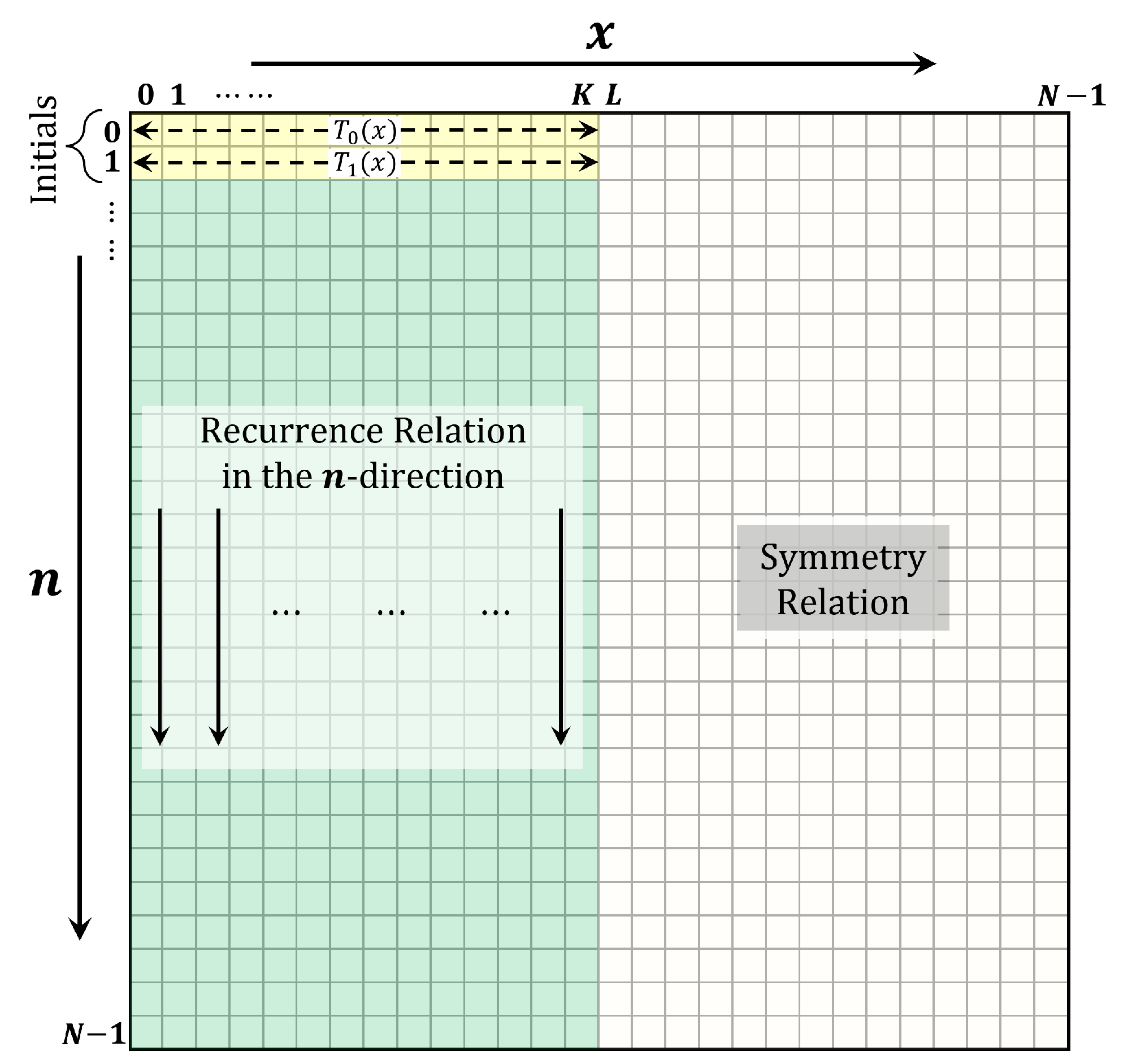
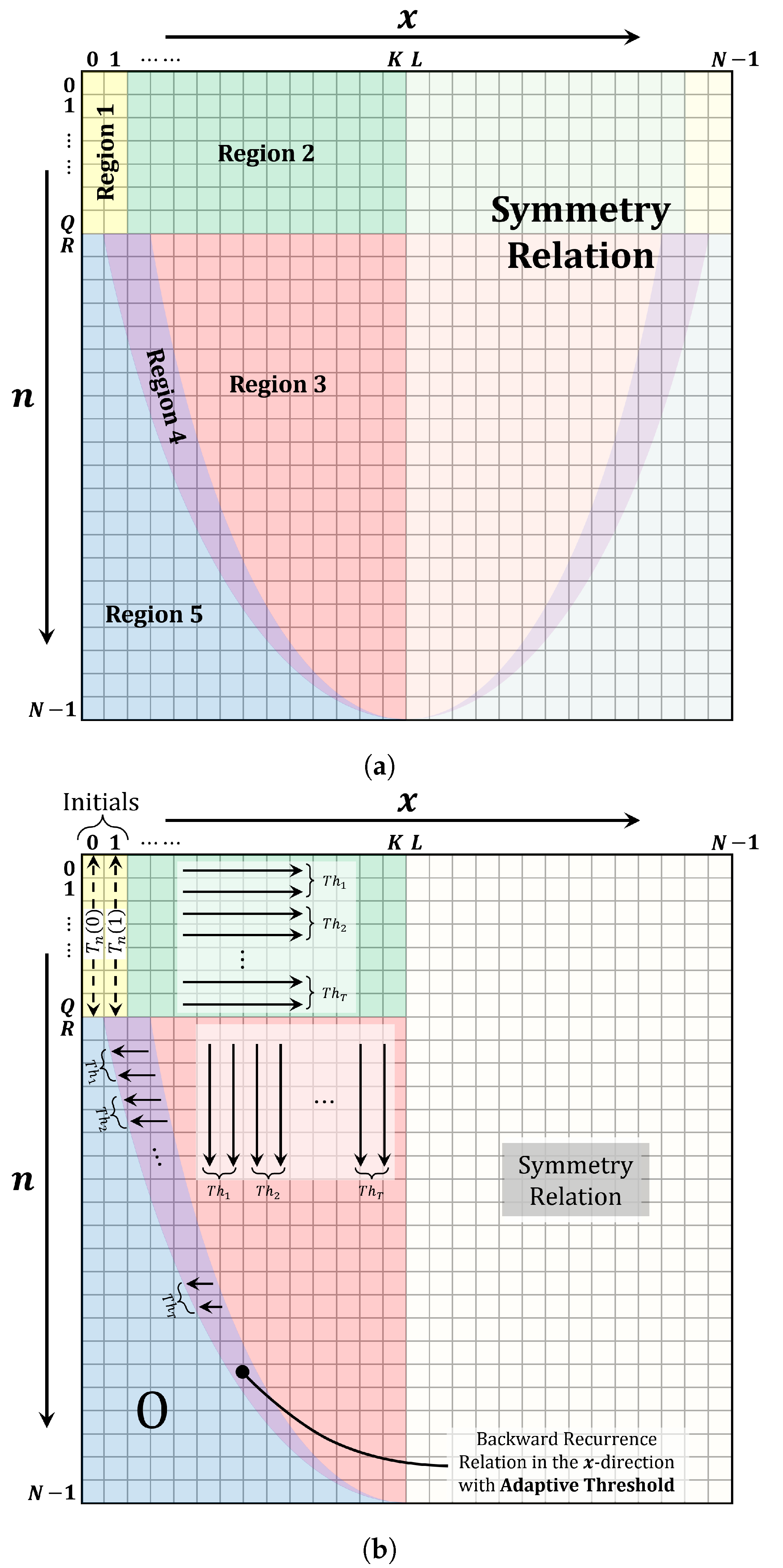
This section provides a detailed explanation of the proposed algorithm, which efficiently computes Tchebichef polynomials by leveraging multithreading and a recurrence approach.

By migrating single-thread processing to multithreading processing, we adopt parallel execution and multithread-based fast TP coefficient calculation for the large-scale dimensional problem. We are able to achieve parallelization, where multiple threads execute distinct tasks concurrently, utilizing multiple processing cores or resources. We have identified the independence of the recurrence relation in coefficient computation, enabling parallelism. This allows threads to be distributed across cores, resulting in accelerated computations through simultaneous execution.

The algorithm begins with Region 1 (see Figure 5), where the aim is to compute the initial sets for the rest of the algorithm. The initial sets are computed over the range $x=0,1$ and $n=0,1,\dots ,Q$. This region is processed in a single thread. To compute these values, the following steps are followed:

• Compute the value of ${\mathcal{T}}_0^N\left(0\right)$ using (17).
• Compute the coefficient values of ${\mathcal{T}}_n^N\left(0\right)$ over the range $x=0$ and $n=1,2,\dots ,Q$ using (18), where $Q={\displaystyle \frac{N}{4}}-1$.
• Compute the value of ${\mathcal{T}}_n^N\left(1\right)$ over the range $x=1$ and $n=0,1,\dots ,Q$ using (19).

Once the computation of the initial sets is carried out, the rest of the polynomials can be computed. In Region 2, the algorithm applies multithreading to process the data in parallel. The number of threads (T) is set, and each thread is assigned a portion of the rows to be processed, which are $T{h}_1$, $T{h}_2$, up to $T{h}_T$. Each thread processes a number of rows, referred to as the bunch size $BS1$, which is calculated as $BS1=(Q+1)/T$. The algorithm uses a recurrence relation in the x-direction for the computation of the values in this region. This means that the computation in this region depends on the previous values of x. By using multithreading, the algorithm can process multiple rows (bunch size) simultaneously, which means speeding up the computation.

In Region 3, the algorithm computes the coefficients using T threads using the TTRR in the x-direction. Each thread is assigned a portion of the columns (bunch size $BS2$) to be processed, the number of columns processed by each thread $BS2=(N/2-L_x)/T$, where $L_x$ is computed using (20). The algorithm uses a recurrence relation in the x-direction for computing the coefficients in this region. This means that the computation in this region depends on the previous coefficient values of x.

In Region 4, the algorithm computes the parameters using multithreading, a recurrence relation in the n-direction, and an adaptive threshold. Each thread is assigned a portion of the rows (bunch size $BS3$) to be processed, with the number of rows processed by each thread $BS3=(N-1-L)/T$, where $L=N/4+1$. The algorithm uses a recurrence relation in the n-direction, but this time in reverse order. This means that the computation in this region depends on the previous values of n, but in a reverse manner. The algorithm also employs an adaptive threshold, which ensures stability of computing the coefficients and detects the first occurrence of instability in the coefficient value at the nth order. The adaptive threshold condition is

$$|{\mathcal{T}}_{n+1}^N(x-1){\displaystyle |}>{\mathcal{T}}_{n+1}^N\left(x\right)$$

(21)

When this condition is true, the coefficients are set to 0 (region 5) and the recurrence relation is stopped at this row. This means that the algorithm effectively prunes the computation. For more elucidation and interpretation, Algorithm 1 provides the pseudo code.

Algorithm 1: The code framework for the proposed multithreaded algorithm.

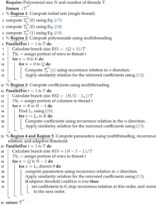
4. Results and Discussion

In this section, we report the results of our experiment, which aimed to improve the speed of generating the Tchebichef polynomials and test the proposed multithreaded algorithm. Specifically, we present the performance metrics and comparative analysis of our approach against existing methods, highlighting the effectiveness of our algorithm in reducing computational time.

The experimental setup consisted of a PC with an eight-core CPU equipped with 16 GB of RAM, utilizing the MS Windows runtime library for multithreading. To thoroughly investigate the impact of thread parallelism on performance, we systematically analyzed the proposed multithreaded algorithms by varying the number of threads in the range {2, 4, 8, 10, 16, 20, 24, 32, 48, 64, 96, 128, 160, 192, 200, 256}. This involves the execution of the proposed algorithm with different threads to take into account how the performance metrics vary in response to increased thread concurrency. Furthermore, we tested the algorithm’s scalability by applying it to a wide range of polynomial sizes, specifically 500, 1000, 2000, 4000, 6000, and 8000, to assess its performance under varying computational loads. It should be noted that each test was repeated 10 times and the average value is reported; this reduces the deviation that may result due to the environment conditions. The evaluation metric involved in this experiment is the improvement ratio in time, i.e., the proposed algorithm execution time to the unthreaded algorithm [33]. The formula of the improvement ratio in time is

$$ImprovementRatio={\displaystyle \frac{UnthreadedTime}{ThreadedTime}}$$

(22)

For a polynomials size of 500 (see Figure 6), the experiment reveals that the algorithm performs best at threads equal to 8, where a speedup improvement of ∼4.2 is achieved. However, as the thread count increases beyond 8, the improvement in speed begins to decrease, indicating diminishing returns due to increased contention for shared resources, synchronization overhead, and scheduling overhead. Moreover, for thread counts above 128, the speedup is less than 1, indicating suboptimal performance due to the indication that the threading management overhead exceeds the timing savings achieved through parallelism. To optimize the algorithm, it is recommended to use 8 threads for a polynomials size of 500.

For a polynomials size of 1000 (see Figure 7), the results indicate that multithreading yields significant performance improvements, with the highest improvement factor of ∼5, which is observed between 8 and 24 threads. This shows that the algorithm is highly parallelizable and that the addition of multiple threads can effectively utilize the available processing resources. However, as the number of threads increases beyond 20, the improvement factor begins to decrease. This is due to the overhead of thread management and synchronization, which becomes more pronounced at higher thread counts. Notably, the improvement factor starts to drop significantly at 128 threads and beyond, showing that the algorithm is no longer able to effectively utilize the additional processing resources. This limitation is likely caused by the hardware’s inability to handle the increased thread count, or the task’s inherent sequential nature, which is also evident in the results for the case where the size was 500.

For a polynomials size of 2000, the multithreading performance analysis depicts a significant improvement in execution time as the number of threads increases, with a peak improvement ratio of 5.73, which is observed at 24 threads (see Figure 8). This demonstrates that the multithreading algorithm is highly parallelizable, effectively utilizing available processing resources. However, as thread count exceeds 48, the improvement factor decreases, which is due to thread management and synchronization overhead. The optimal thread count lies between 16 and 48, where the improvement factor is highest. Notably, the improvement factor drops to 3.19 at 256 threads, indicating that excessive threading leads to decreased performance.

This stable improvement at a high number of threads is due to the fact that the computational loads are high, leading to diminishing threading overheads. This is clear from the improvement achieved at 256 threads, where it drops to 17.9% and 27.4% from the optimal improvement at size of 500 and 1000, respectively. At a size of 2000, the improvement in 256 threads decreases to 55.7% with respect to the maximum improvement.

The results for a size of 4000 and 6000 are depicted in Figure 9 and Figure 10. The experiment shows that the thread-scaling results exhibit a nonlinear relationship between thread count and improvement. This is characterized by a rapid increase in improvement up to 16 threads, where a plateau is reached. The improvement then continues to increase, reaching the peak at ∼20 threads, before a subsequent decline.

This behavior is attributed to the interplay between parallelism and overhead, where the benefits of parallelism are initially dominant. The optimal thread count corresponds to an inflection point where the parallelism benefits are maximized and the overhead is minimized, with the maximum improvement occurring in the region between 16 and 64 threads for a size of 4000 and between 16 and 96 threads for a size of 6000. However, eventually, the benefits of parallelism give way to the increasing overhead of thread creation, synchronization, and communication, leading to diminishing returns after 64 threads for a size of 4000 and after 96 threads for a size of 6000.

For a size of 8000, the results shown in Figure 11 reveal that the improvement in performance increases and reaches the optimal thread with a maximum improvement of 7.22 at 32 threads. Beyond this point, the improvement values start to decline, indicating that the overhead costs of thread creation, synchronization, and communication begin to dominate, leading to diminishing returns. The optimal number for this case occurs at thread count 16 to 96.

Based on the observed results of the conducted experiments, the number of threads that achieves the maximum improvement is different for each size and does not follow a linear relation. The highest improvements are observed in a range of threads, especially in the sizes 4000 to 8000, with a very slight difference between them. For example, at size = 4000, the highest improvement was achieved in the range of 16 to 64 threads. It should be noted that the results represent the average of 10 executions to reduce the deviations; despite that, the environment conditions, namely the other tasks running in the background, have some effect on the experimental results, leading to this non-linearity.

The experimental results for the sizes of 4000, 6000, and 8000 show that the improvement at 256 threads drops to only 87.4%, 89.9%, and 90.3% from the peak improvement value at a size of 4000, 6000, and 8000, respectively.

The improvement through threading is dependent on the available computing resources, represented by the number of cores. Figure 12 shows the calculation improvement as a function of the number of threads for different numbers of cores, namely one, two, three, and four cores. In general, the improvement increases with an increase in the number of cores. The one-core case shows small improvement at a small number of threads for sizes 500, 1000, and 2000, and this improvement falls below 1 at higher numbers of threads, which indicates a degradation. A high number of threads at small sizes (500 and 1000) leads to diminishing returns due to the threading overhead, and this applies to all of the numbers of cores considered. At larger sizes of 2000 and above, the results achieved by two or more cores show more improvement stability. The maximum improvement achieved by the two-core case is 4.4 at 32 threads at the 8000 size. On the other hand, the three-core case achieved an up to 5.79 improvement at 24 threads at the 8000 size. Clearly, the proposed algorithm, using multicore and multithreaded parallel TPs calculations, addresses the issue of long calculation times for large-scale dimensions. Not only does it solve this problem but it also improves the stability and accuracy of the solution, resulting in enhanced overall performance.

5. Conclusions

The computation of TPs represents a time-consuming operation, especially in high-order signals. This work proposed an approach to handle large-sized signals with performance enhancement while maintaining numerical stability. The proposed approach distributed the calculation workload among independent threads, thus taking advantage of the available parallel computing resources represented by the multicores. This approach divides the coefficients into four regions, where the first region represents an initialization. Parallelism within each of the three other regions is exploited and the workload is divided between a set of threads that run on the different cores. The proposed approach showed a clear improvement in performance, achieving an improvement of 7.2 times with respect to the unthreaded case. This maximum improvement was obtained at the highest size considered (8000) when the number of threads is set to 32 with 8 cores. It was noticed that increasing the number of threads does not necessarily result in performance improvement. A high number of threads introduces management overheads that, at some point, diminish the speedup of parallel execution. This was clear in all sizes considered, but it was especially prominent at small sizes, namely 500 and 1000, where the improvement drops to 17.9% and 24.7% of the maximum improvement achieved. Multithreading-based TPs computation provides faster and more accurate calculations and brings new opportunities to algorithm designers. Moreover, implementing multithreaded-strategy-based orthogonal polynomial computations will be one of the important future directions in accelerating the computations in the field of signal processing.

References

1. Abd-Elhameed, W.M.; Al-Harbi, M.S. Some formulas and recurrences of certain orthogonal polynomials generalizing Chebyshev polynomials of the third-kind. Symmetry 2022, 14, 2309. [Google Scholar] [CrossRef]
2. Sun, L.; Chen, Y. Numerical analysis of variable fractional viscoelastic column based on two-dimensional Legendre wavelets algorithm. Chaos Solitons Fractals 2021, 152, 111372. [Google Scholar] [CrossRef]
3. AbdelFattah, H.; Al-Johani, A.; El-Beltagy, M. Analysis of the stochastic quarter-five spot problem using polynomial chaos. Molecules 2020, 25, 3370. [Google Scholar] [CrossRef]
4. Alhaidari, A.D.; Taiwo, T. Energy spectrum design and potential function engineering. Theor. Math. Phys. 2023, 216, 1024–1035. [Google Scholar] [CrossRef]
5. Yang, J.; Zeng, Z.; Kwong, T.; Tang, Y.Y.; Wang, Y. Local Orthogonal Moments for Local Features. IEEE Trans. Image Process. 2023, 32, 3266–3280. [Google Scholar] [CrossRef]
6. Markel, J.; Gray, A. Roundoff noise characteristics of a class of orthogonal polynomial structures. IEEE Trans. Acoust. Speech Signal Process. 1975, 23, 473–486. [Google Scholar] [CrossRef]
7. Ma, R.; Shi, L.; Huang, Z.; Zhou, Y. EMP signal reconstruction using associated-Hermite orthogonal functions. IEEE Trans. Electromagn. Compat. 2014, 56, 1242–1245. [Google Scholar] [CrossRef]
8. Abdulhussain, S.H.; Mahmmod, B.M.; Flusser, J.; AL-Utaibi, K.A.; Sait, S.M. Fast overlapping block processing algorithm for feature extraction. Symmetry 2022, 14, 715. [Google Scholar] [CrossRef]
9. Abdulqader, D.A.; Hathal, M.S.; Mahmmod, B.M.; Abdulhussain, S.H.; Al-Jumeily, D. Plain, edge, and texture detection based on orthogonal moment. IEEE Access 2022, 10, 114455–114468. [Google Scholar] [CrossRef]
10. Levenshtein, V.I. Krawtchouk polynomials and universal bounds for codes and designs in Hamming spaces. IEEE Trans. Inf. Theory 1995, 41, 1303–1321. [Google Scholar] [CrossRef]
11. Zeng, J. Linearization of Meixner, Krawtchouk, and Charlier polynomial products. SIAM J. Math. Anal. 1990, 21, 1349–1368. [Google Scholar] [CrossRef]
12. Karakasis, E.G.; Papakostas, G.A.; Koulouriotis, D.E.; Tourassis, V.D. Generalized dual Hahn moment invariants. Pattern Recognit. 2013, 46, 1998–2014. [Google Scholar] [CrossRef]
13. Mahmmod, B.M.; Flayyih, W.N.; Fakhri, Z.H.; Abdulhussain, S.H.; Khan, W.; Hussain, A. Performance enhancement of high order Hahn polynomials using multithreading. PLoS ONE 2023, 18, e0286878. [Google Scholar] [CrossRef]
14. Zhu, H.; Shu, H.; Liang, J.; Luo, L.; Coatrieux, J.L. Image analysis by discrete orthogonal Racah moments. Signal Process. 2007, 87, 687–708. [Google Scholar] [CrossRef]
15. Mahmmod, B.M.; Abdulhussain, S.H.; Suk, T.; Alsabah, M.; Hussain, A. Accelerated and improved stabilization for high order moments of Racah polynomials. IEEE Access 2023, 11, 110502–110521. [Google Scholar] [CrossRef]
16. Veerasamy, M.; Jaganathan, S.C.B.; Dhasarathan, C.; Mubarakali, A.; Ramasamy, V.; Kalpana, R.; Marina, N. Legendre Neural Network Method for Solving Nonlinear Singular Systems. In Intelligent Technologies for Sensors; Apple Academic Press: Palm Bay, FL, USA, 2023; pp. 25–37. [Google Scholar]
17. Boelen, L.; Filipuk, G.; Van Assche, W. Recurrence coefficients of generalized Meixner polynomials and Painlevé equations. J. Phys. A Math. Theor. 2010, 44, 035202. [Google Scholar] [CrossRef]
18. Vasileva, M.; Kyurkchiev, V.; Iliev, A.; Rahnev, A.; Kyurkchiev, N. Associated Hermite Polynomials. Some Applications. Int. J. Differ. Equ. Appl. 2023, 22, 1–17. [Google Scholar]
19. Schweizer, W.; Schweizer, W. Laguerre Polynomials. In Special Functions in Physics with MATLAB; Springer: Cham, Switzerland, 2021; pp. 211–214. [Google Scholar]
20. Mukundan, R.; Ong, S.; Lee, P. Image analysis by Tchebichef moments. IEEE Trans. Image Process. 2001, 10, 1357–1364. [Google Scholar] [CrossRef]
21. Li, J.; Wang, P.; Ni, C.; Zhang, D.; Hao, W. Loop Closure Detection for Mobile Robot based on Multidimensional Image Feature Fusion. Machines 2022, 11, 16. [Google Scholar] [CrossRef]
22. Teague, M.R. Image analysis via the general theory of moments. J. Opt. Soc. Am. 1980, 70, 920–930. [Google Scholar] [CrossRef]
23. Jahid, T.; Karmouni, H.; Hmimid, A.; Sayyouri, M.; Qjidaa, H. Fast computation of Charlier moments and its inverses using Clenshaw’s recurrence formula for image analysis. Multimed. Tools Appl. 2019, 78, 12183–12201. [Google Scholar] [CrossRef]
24. den Brinker, A.C. Stable calculation of Krawtchouk functions from triplet relations. Mathematics 2021, 9, 1972. [Google Scholar] [CrossRef]
25. den Brinker, A.C. Stable Calculation of Discrete Hahn Functions. Symmetry 2022, 14, 437. [Google Scholar] [CrossRef]
26. Aldakheel, E.A.; Khafaga, D.S.; Fathi, I.S.; Hosny, K.M.; Hassan, G. Efficient Analysis of Large-Size Bio-Signals Based on Orthogonal Generalized Laguerre Moments of Fractional Orders and Schwarz–Rutishauser Algorithm. Fractal Fract. 2023, 7, 826. [Google Scholar] [CrossRef]
27. Costas-Santos, R.S.; Soria-Lorente, A.; Vilaire, J.M. On Polynomials Orthogonal with Respect to an Inner Product Involving Higher-Order Differences: The Meixner Case. Mathematics 2022, 10, 1952. [Google Scholar] [CrossRef]
28. Fernández-Irisarri, I.; Mañas, M. Pearson equations for discrete orthogonal polynomials: II. Generalized Charlier, Meixner and Hahn of type I cases. arXiv 2021, arXiv:2107.02177. [Google Scholar]
29. Bourzik, A.; Bouikhalen, B.; El-Mekkaoui, J.; Hjouji, A. A comparative study and performance evaluation of discrete Tchebichef moments for image analysis. In Proceedings of the 6th International Conference on Networking, Intelligent Systems & Security, Larache, Morocco, 24–26 May 2023; pp. 1–7. [Google Scholar]
30. Mukundan, R. Some Computational Aspects of Discrete Orthonormal Moments. IEEE Trans. Image Process. 2004, 13, 1055–1059. [Google Scholar] [CrossRef]
31. Abdulhussain, S.H.; Ramli, A.R.; Al-Haddad, S.A.R.; Mahmmod, B.M.; Jassim, W.A. On Computational Aspects of Tchebichef Polynomials for Higher Polynomial Order. IEEE Access 2017, 5, 2470–2478. [Google Scholar] [CrossRef]
32. Camacho-Bello, C.; Rivera-Lopez, J.S. Some computational aspects of Tchebichef moments for higher orders. Pattern Recognit. Lett. 2018, 112, 332–339. [Google Scholar] [CrossRef]
33. Abdulhussain, S.H.; Mahmmod, B.M.; Baker, T.; Al-Jumeily, D. Fast and accurate computation of high-order Tchebichef polynomials. Concurr. Comput. Pract. Exp. 2022, 34, e7311. [Google Scholar] [CrossRef]
34. Kumar, R.; Tullsen, D.M.; Jouppi, N.P. Core architecture optimization for heterogeneous chip multiprocessors. In Proceedings of the 15th International Conference on Parallel Architectures and Compilation Techniques, Seattle, WA, USA, 16–20 September 2006; pp. 23–32. [Google Scholar]
35. Schildermans, S.; Shan, J.; Aerts, K.; Jackrel, J.; Ding, X. Virtualization overhead of multithreading in X86 state-of-the-art & remaining challenges. IEEE Trans. Parallel Distrib. Syst. 2021, 32, 2557–2570. [Google Scholar]
36. Thomadakis, P.; Tsolakis, C.; Chrisochoides, N. Multithreaded runtime framework for parallel and adaptive applications. Eng. Comput. 2022, 38, 4675–4695. [Google Scholar] [CrossRef]
37. Kim, E.; Choi, S.; Kim, C.G.; Park, W.C. Multi-Threaded Sound Propagation Algorithm to Improve Performance on Mobile Devices. Sensors 2023, 23, 973. [Google Scholar] [CrossRef] [PubMed]
38. Wei, X.; Ma, L.; Zhang, H.; Liu, Y. Multi-core-, multi-thread-based optimization algorithm for large-scale traveling salesman problem. Alex. Eng. J. 2021, 60, 189–197. [Google Scholar] [CrossRef]
39. Luan, G.; Pang, P.; Chen, Q.; Xue, S.; Song, Z.; Guo, M. Online thread auto-tuning for performance improvement and resource saving. IEEE Trans. Parallel Distrib. Syst. 2022, 33, 3746–3759. [Google Scholar] [CrossRef]
40. Donoho, D.L. Compressed sensing. IEEE Trans. Inf. Theory 2006, 52, 1289–1306. [Google Scholar] [CrossRef]
41. Abramowitz, M.; Stegun, I.A. Handbook of Mathematical Functions: With Formulas, Graphs, and Mathematical Tables; Dover Publications: New York, NY, USA, 1964. [Google Scholar]
42. Foncannon, J.J. Irresistible integrals: Symbolics, analysis and experiments in the evaluation of integrals. Math. Intell. 2006, 28, 65–68. [Google Scholar] [CrossRef]
43. Gautschi, W. Computational aspects of three-term recurrence relations. SIAM Rev. 1967, 9, 24–82. [Google Scholar] [CrossRef]
44. Lewanowicz, S. Recurrence relations for hypergeometric functions of unit argument. Math. Comput. 1985, 45, 521–535. [Google Scholar] [CrossRef]
Figure 1. The steps used to compute the TPs coefficients using TTRRn.
Algorithms 17 00381 g001
Figure 2. The steps used to compute the TPs coefficients using TTRRx.
Algorithms 17 00381 g002
Figure 3. The steps of the TTRRnx algorithm.
Algorithms 17 00381 g003
Figure 4. The steps of the sequential TTRRnxa algorithm.
Algorithms 17 00381 g004
Figure 5. Multithreading-based algorithm for fast TTRRnxa calculation. (a) Regions of the multithreaded algorithm, and (b) distribution of the threads in the multithreaded algorithm.
Algorithms 17 00381 g005
Figure 6. The computation time and speedup of the proposed algorithm for size of 500.
Algorithms 17 00381 g006
Figure 7. Computation time and performance gain of the proposed algorithm for size 1000.
Algorithms 17 00381 g007
Figure 8. The computation time and speedup of the proposed algorithm for size of 2000.
Algorithms 17 00381 g008
Figure 9. Computation time and performance gain of the proposed algorithm for size 4000.
Algorithms 17 00381 g009
Figure 10. The computation time and speedup of the proposed algorithm for size of 6000.
Algorithms 17 00381 g010
Figure 11. Computation time and performance gain of the proposed algorithm for size 8000.
Algorithms 17 00381 g011
Figure 12. Improvement of the Multithreaded algorithm as a function of the number of threads for different numbers of cores and for sizes: (a) 500, (b) 1000, (c) 2000, (d) 4000, (e) 6000, and (f) 8000.
Algorithms 17 00381 g012
Disclaimer/Publisher’s Note: The statements, opinions and data contained in all publications are solely those of the individual author(s) and contributor(s) and not of MDPI and/or the editor(s). MDPI and/or the editor(s) disclaim responsibility for any injury to people or property resulting from any ideas, methods, instructions or products referred to in the content.