Abstract
Parallel optimization enables faster and more efficient problem-solving by reducing computational resource consumption and time. By simultaneously combining multiple methods, such as evolutionary algorithms and swarm-based optimization, effective exploration of the search space and achievement of optimal solutions in shorter time frames are realized. In this study, a combination of termination criteria is proposed, utilizing three different criteria to end the algorithmic process. These criteria include measuring the difference between optimal values in successive iterations, calculating the mean value of the cost function in each iteration, and the so-called “DoubleBox” criterion, which is based on the relative variance of the best value of the objective cost function over a specific number of iterations. The problem is addressed through the parallel execution of three different optimization methods (PSO, Differential Evolution, and Multistart). Each method operates independently on separate computational units with the goal of faster discovery of the optimal solution and more efficient use of computational resources. The optimal solution identified in each iteration is transferred to the other computational units. The proposed enhancements were tested on a series of well-known optimization problems from the relevant literature, demonstrating significant improvements in convergence speed and solution quality compared to traditional approaches.
1. Introduction
The problem of finding the global minimum of a multidimensional function occurs in various scientific areas and has wide applications. In this context, the programmer seeks the absolute minimum of a function subject to some assumptions or constraints. The objective function is defined as and the mathematical formulation of the global optimization problem is as follows:
where the set S is as follows:
Such problems frequently arise in sciences like physics, where genetic algorithms prove effective in locating positions in magnetic plasmas and in developing optimization tools [1]. Additionally, the combined use of various optimization techniques enhances performance and stability in complex problems [2]. Furthermore, the hybrid approach that combines artificial physics techniques with particle swarm optimization has proven to be particularly effective in solving energy allocation problems [3]. In the field of chemistry, minimizing potential energy functions is crucial for understanding the ground states of molecular clusters and proteins [4]. Optimizing these functions has been used for accurate protein structure prediction, with results closely matching crystal structures [5]. Moreover, a new computational framework combining variance-based methods with artificial neural networks has significantly improved accuracy and reduced computational cost in sensitivity analyses [6]. Even in the field of economics, optimization plays a crucial role. The particle swarm optimization (PSO) method is shown to be highly effective in solving the economic dispatch problem in power systems, providing higher quality solutions with greater efficiency compared to genetic algorithms [7]. Additionally, a multi-objective optimization approach for economic load dispatch and emission reduction in hydroelectric and thermal plants achieves optimal solutions that align with the user’s preferences and goals [8]. Finally, optimization is also applied in biological process models [9] and medical data classification, achieving high accuracy in diagnosing diseases and analyzing genomes [10]. A series of methods have been proposed in the recent literature to handle problems described by Equation (1). Methods used to handle problems described by Equation (1) are usually divided into two categories: deterministic and stochastic methods. In the first category, the most common method is the interval method [11,12], where the set S is divided through a series of steps into subregions and some subregions that do not contain the global solution can be removed using some pre-defined criteria. The second category contains stochastic techniques that do not guarantee finding the total minimum, and they are easier to program since they do not rely on some assumptions about the objective function. In addition, they also constitute the vast majority of global optimization methods. Among them, there are methods based on considerations derived from Physics, such as the Simulated Annealing method [13], the Henry’s Gas Solubility Optimization (HGSO) [14], the Gravitational Search Algorithm (GSA) [15], the Small World Optimization Algorithm (SWOA) [16], etc. Also, a series of evolutionary-based techniques have also been suggested for Global Optimization problems, such as Genetic Algorithms [17], the Differential Evolution method [18,19], Particle Swarm Optimization (PSO) [20,21], Ant Colony Optimization (ACO) [22], Bat Algorithm (BA) [23], Whale Optimization Algorithm (WOA) [24], Grasshopper Optimization Algorithm (GOA) [25], etc.
However, the above optimization methods require significant computational power and time. Therefore, parallel processing of these methods is essential. Recently, various methods have been proposed to leverage parallel processing. Specifically, one study details the parallel implementation of the Particle Swarm Optimization (PSO) algorithm, which improves performance for load-balanced problems but shows reduced efficiency for load-imbalanced ones. The study suggests using larger particle populations and implementing asynchronous processing to enhance performance [26]. Another review provides a comprehensive overview of derivative-free optimization methods, useful for problems where objective and constraint functions come only from a black-box or simulator interface. The review focuses on recent developments and categorizes methods based on assumptions about functions and their characteristics [27]. Lastly, the PDoublePop version 1.0 software is presented, which implements parallel genetic algorithms with advanced features, such as an enhanced stopping rule and advanced mutation schemes. The software allows for coding the objective function in C++ or Fortran77 and has been tested on well-known benchmark functions, showing promising results [28]. Moreover, there are methods that utilize GPU architectures for solving complex optimization problems. In the case of the Traveling Salesman Problem (TSP), a parallel GPU implementation has been developed to achieve high performance on large scales, solving problems of up to 6000 cities with great efficiency [29]. Additionally, the use of the multi-start model in local search algorithms has proven to be particularly effective when combined with GPUs, reducing computation time and improving solution quality for large and time-intensive problems [30]. Finally, a parallel algorithm using Peano curves for dimension reduction has demonstrated significant improvements in speed and efficiency when run on GPUs, compared to CPU-only implementations, for multidimensional problems with multiple local minima [31]. Parallel optimization represents a significant approach in the field of optimization problem-solving and is applied across a broad range of applications, including the optimization of machine learning model parameters. In the case of GraphLab, a platform is presented that enhances existing abstract methods, such as MapReduce, for parallel execution of machine learning algorithms with high performance and accuracy [32]. Additionally, the new MARSAOP method for hyperparameter optimization uses multidimensional spirals as surrogates and dynamic coordinate search to achieve high-quality solutions with limited computational costs [33]. Lastly, the study proposes a processing time-estimation system using machine learning models to adapt to complex distributions and improve production scheduling, achieving significant reduction in completion time [34].
The use of parallel optimization has brought significant advancements in solving complex control and design problems [35]. In one case, the parallel application of the Genetic Algorithm with a Fair Competitive Strategy (HFCGA) has been used for the design of an optimized cascade controller for ball and beam systems. This approach allows for the automation of controller parameter tuning, improving performance compared to traditional methods, with parallel computations helping to avoid premature convergence to suboptimal solutions [36]. In another case, the advanced Teaching–Learning-Based Optimization (TLBO) method has been applied to optimize the design of propulsion control systems with hydrogen peroxide. This method, which includes improvements in the teaching and learning phases as well as in the search process, has proven highly effective in addressing uncertainties in real-world design problems, enhancing both accuracy and convergence speed of the optimization process [37].
Similarly, parallel optimization has significant applications in energy and resource management. In the case of pump and cooling system management, a two-stage method based on an innovative multidimensional optimization algorithm has been proposed, which reduces overall energy consumption and discrepancies between pump and cooling system flow rates, achieving significant improvements in energy efficiency [38]. In energy network management, a coordinated scheduled optimization method has been proposed, which simultaneously considers various energy sources and uncertainty conditions. This method, using the Competitive Swarm Optimization (CSO) algorithm and adjusted based on chaos theory, has proven 50% faster than other methods and effective in managing uncertainties and energy [39]. In topological optimization, parallel processing through CPUs and GPUs has drastically improved speed and energy consumption for complex problems, achieving up to 25-times faster processing and reducing energy consumption by up to 93% [40]. Lastly, in building energy retrofitting, a multi-objective platform was used for evaluating and optimizing upgrade strategies, demonstrating that removing subsidies and providing incentives for energy upgrades yield promising results [41].
In conclusion, parallel optimization has provided significant solutions to problems related to sustainable development and enhancing sustainability. In the field of increasing the resilience of energy systems, the development of strategies for managing severe risks, such as extreme weather conditions and supplier disruptions, has been improved through parallel optimization, enabling safer and more cost-effective energy system operations [42]. In addressing groundwater contamination, the use of parallel optimization has highlighted the potential for faster and more effective design of remediation methods, significantly reducing computational budgets and ensuring better results compared to other methods [43]. Finally, in the field of sustainable production, metaheuristic optimization algorithms have proven useful for improving production scheduling, promoting resource efficiency, and reducing environmental impacts, while contributing to the achievement of sustainable development goals [44].
By harnessing multiple computational resources, parallel optimization allows for the simultaneous execution of multiple algorithms, leading to faster convergence and improved performance. These computational resources can communicate with each other to exchange information and synchronize processes, thereby contributing to faster convergence towards common solutions. Additionally, leveraging multiple resources enables more effective handling of exceptions and errors, while increased computational power for conducting more trials or utilizing more complex models leads to enhanced performance [45]. Of course, this process requires the development of suitable algorithms and techniques to effectively manage and exploit available resources. Each parallel optimization algorithm requires a coherent strategy for workload distribution among the available resources, as well as an efficient method for collecting and evaluating results.
Various researchers have developed parallel techniques, such as the development and evaluation of five different parallel Simulated Annealing (SA) algorithms for solving global optimization problems. The paper compares the performance of these algorithms across an extensive set of tests, focusing on various synchronization and information exchange approaches, and highlights their particularly noteworthy performance on functions with large search spaces where other methods have failed [46]. Additionally, other research focuses on the parallel application of the Particle Swarm Optimization (PSO) method, analyzing the performance of the parallel PSO algorithm on two categories of problems: analytical problems with low computational costs and industrial problems with high computational costs [47]. This research demonstrates that the parallel PSO method performs exceptionally well on problems with evenly distributed loads, while in cases of uneven loads, the use of asynchronous approaches and larger particle populations proves more effective. Another study develops a parallel implementation of a stochastic Radial Basis Function (RBF) algorithm for global optimization, which does not require derivatives and is suitable for computationally intensive functions. The paper compares the performance of the proposed method with other parallel optimization methods, noting that the RBF method achieves good results with one, four, or eight processors across various optimization problems [48]. Parallel techniques are also applied in real-time image processing, which is critical for applications such as video surveillance, diagnostic medicine, and autonomous vehicles. A related article examines parallel architectures and algorithms, identifying effective applications and evaluating the challenges and limitations of their practical implementation, aiming to develop more efficient solutions [49]. Another study reviews parallel computing strategies for computational fluid dynamics (CFD), focusing on tools like OpenMP, MPI, and CUDA to reduce computational time [50]. Finally, a significant study explores parallel programming technologies for processing genetic sequences, presenting three main parallel computing models and analyzing applications such as sequence alignment, single nucleotide polymorphism calling, sequence preprocessing, and pattern detection [51].
Genetic Algorithms (GAs) are methods that can be easily parallelized, and several researchers have thoroughly examined them in the literature. For example, a universal parallel execution method for Genetic Algorithms, known as IIP (Parallel, Independent, and Identical Processing), is presented. This method achieves acceleration with the use of m processors. The technique calculates execution speed and compares results on small-size problems and the non-parametric Inverse Fractal Problem [52]. Similarly, another paper presents a distributed mechanism for improving resource protection in a digital ecosystem. This mechanism can be used not only for secure and reliable transactions but also to enhance collaboration among digital ecosystem community members to secure the environment, and also employs Public Key Infrastructure to provide strong protection for access workflows [53]. Genetic Algorithms have also been used as a strategy for optimizing large and complex problems, specifically in wavelength selection for multi-component analysis. The study examines the effectiveness of the genetic algorithm in finding acceptable solutions in a reasonable time and notes that the algorithm incorporates prior information to improve performance, based on mathematically grounded frameworks such as the schema theorem [54]. Additionally, another paper develops two genetic algorithm-based algorithms to improve the lifetime and energy consumption in mobile wireless sensor networks (MWSNs). The first algorithm is an improvement of the Unequal Clustering Genetic Algorithm, while the second algorithm combines the K-means Clustering Algorithm with Genetic Algorithms. These algorithms aim to better adapt to dynamic changes in network topology, thereby enhancing network lifetime and energy consumption [55]. Lastly, the use of Genetic Algorithms has promising applications across various medical specialties, including radiology, radiotherapy, oncology, pediatrics, cardiology, endocrinology, surgery, obstetrics and gynecology, pulmonology, infectious diseases, orthopedics, rehabilitation medicine, neurology, pharmacotherapy, and health care management. A related paper reviews and introduces applications of Genetic Algorithms in disease screening, diagnosis, treatment planning, pharmacovigilance, prognosis, and health care management, enabling physicians to envision potential applications of this metaheuristic method in their medical careers [56].
In this paper, a new optimization method is proposed which is a mixture of existing global optimization techniques running in parallel on a number of available computing units. Each technique is executed independently of the others and periodically the optimal values retrieved from them are distributed to the rest of the computing units using the propagation techniques presented here. In addition, for the most efficient termination of the overall algorithm, intelligent termination techniques based on stochastic observations are used, which are suitably modified to adapt to the parallel computing environment. The contributions of this work as summarized as follows:
- Periodic local search was integrated into the Differential Evolution (DE) and Particle Swarm Optimization (PSO) methods.
- A mechanism for disseminating the optimal solution to all PUs was added in each iteration of the methods.
- The overall algorithm terminates based on the proposed termination criterion.
The following sections are organized as follows: In Section 2, the three main algorithms participating in the overall algorithm are described. In Section 3 the algorithm for parallelizing the three methods is described, along with the proposed mechanism for propagating the optimal solution to the remaining methods. In Section 4, experimental models and experimental results are described. Finally, in Section 5, the conclusions from the application of the current work are discussed.
2. Adopted Algorithms
The methods executed in each processing unit are fully described in this section.
2.1. The Method PSO
PSO is an optimization method inspired by the behavior of swarms in nature. In PSO, a set of particles moves in the search space seeking the optimal solution. Each particle has a current position and velocity, and it moves based on its past performance and that of its neighboring particles. PSO continuously adjusts the movement of particles, aiming for convergence to the optimal solution [57,58,59]. This method can be programmed easily and the set of the parameters to be set is limited. Hence, it has been used in a series of practical problems, such as problems that arise in physics [60,61], chemistry [62,63], medicine [64,65], economics [66], etc. The main steps of the PSO method are presented in Algorithm 1.
| Algorithm 1 The main steps of the PSO method |
|
2.2. The Method Differential Evolution
The DE method relies on differential operators and is particularly effective in optimization problems that involve searching through a continuous search space. By employing differential operators, DE generates new solutions that are then evaluated and adjusted until the optimal solution is achieved [67,68]. The method was used in a series of problems, such as electromagnetics [69], energy consumption problems [70], job shop scheduling [71], image segmentation [72], etc. The Differential Evolution operates through the following steps: Initially, initialization takes place with a random population of solutions in the search space. Then, each solution is evaluated based on the objective function. Subsequently, a process is iterated involving the generation of new solutions through modifications, evaluation of these new solutions, and selection of the best ones for the next generation. The algorithm terminates when a termination criterion is met, such as achieving sufficient improvement in performance or exhausting the number of iterations. The main steps of the DE method are presented in Algorithm 2.
| Algorithm 2 The main steps of the DE method |
|
2.3. The Method Multistart
In contrast, the Multistart method follows a different approach than previous methods. Instead of focusing on a single initial point, it repeats the search from various initial points in the search space. This allows for a broader exploration of the search space and increases the chances of finding the optimal solution. The Multistart method is particularly useful when optimization algorithms may get trapped in local minima [73,74,75]. The approach of multiple starts belongs to the simplest techniques for global optimization. At the outset of the process, an initial distribution of points is made in Euclidean space. Subsequently, local optimization begins simultaneously from these points. The discovered minima are compared, and the best one is retained as the global minimum. Local optimizations rely on the Broyden Fletcher Goldfarb Shanno (BFGS) method [76]. The main steps of the multistart method are presented in Algorithm 3.
| Algorithm 3 The main steps of the Multistart method |
|
3. The Proposed Method
In the present work, a mixture of termination rules is proposed as a novel technique, which can be used without partitioning in any stochastic global optimization technique. Also, a new parallel global optimization technique is proposed that utilizes the new termination rule.
The existing method that was presented in Section 2, employs Particle Swarm Optimization (PSO), Differential Evolution (DE), and Multistart techniques, each with its own independent termination criteria. In contrast, the proposed method that will be presented in this section integrates an innovative combination of termination rules, including Best-Fitness, Mean-Fitness, and DoubleBox, enhancing the termination process of the search. By incorporating these advanced termination strategies into a parallel algorithm, the new method achieves faster convergence and improved solution quality. This approach combines the efficiency of parallel execution with the flexibility of advanced termination criteria, representing a significant advancement over traditional methods. In the following subsections, the new termination rule is fully described, followed by the new optimization method.
3.1. The New Termination Rule
The proposed termination rule is a mixture of several stochastic termination rules proposed in the recent literature. The first algorithm will be called best—fitness and in this termination technique, at each iteration k, the difference between the current best value and the previous best value is calculated [77], i.e., the absolute difference:
If this difference is zero for a series of predefined consecutive iterations , then the method terminates. In the second termination rule, which will be called mean—fitness, the average function value for each iteration is computed. If this value remains relatively unchanged over a certain number of consecutive iterations, it indicates that the method may not be making significant progress towards discovering a new global minimum. Therefore, termination is warranted [19]. Hence, in every iteration k, we compute:
The value denotes the number of particles or chromosomes that participate in the algorithm. The termination rule is defined as follows: terminate if for a predefined number of iterations. The third stopping rule is the so-called DoubleBox stopping rule, which was initially proposed in the work of Tsoulos [78]. In this criterion, the search process is terminated once sufficient coverage of the search space has been achieved. The estimation of the coverage is based on the asymptotic approximation of the relative proportion of points that lead to local minima. Since the exact coverage cannot be directly calculated, sampling is conducted over a larger region. The search is stopped when the variance of the sample distribution falls below a predefined threshold, which is adjusted based on the most recent discovery of a new local minimum. According to this criterion, the algorithm terminates when one of the following conditions is met:
- The iteration k count exceeds a predefined limit of iterations ;
- The relative variance falls below half of the variance of the last iteration where a new optimal functional value was found.
3.2. The Proposed Algorithm
In the scientific literature, parallelization typically involves distributing the population among parallel computing units to save computational power and time [77,79]. In the present study, we concurrently compute the optimal solutions of three different stochastic optimization methods originating from different classification categories. The proposed algorithm is shown in Algorithm 4.
| Algorithm 4 The proposed overall algorithm |
|
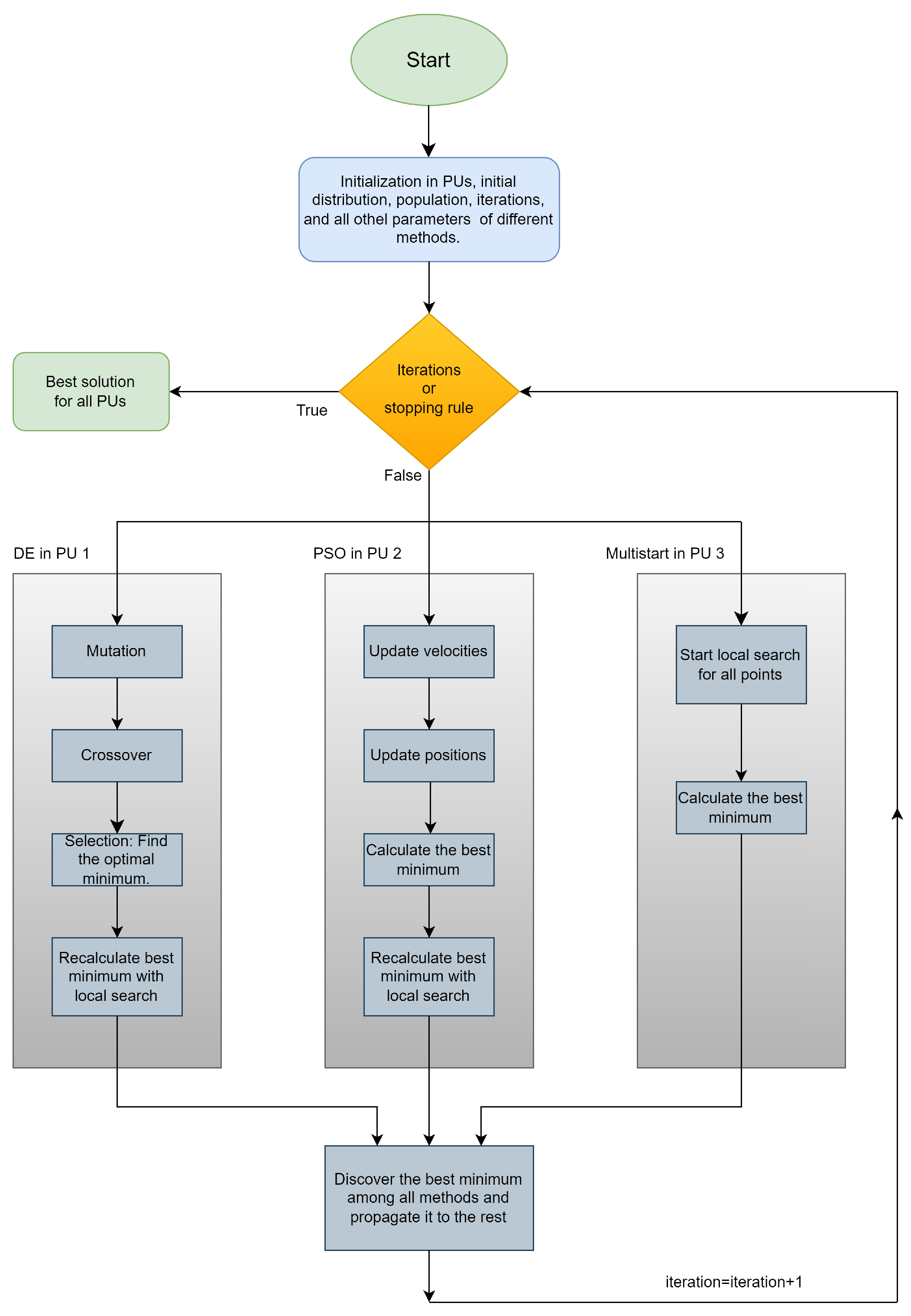
The proposed algorithm is graphically outlined in Figure 1. The methods that are used in each processing unit may include Particle Swarm Optimization, the Multistart method, and Differential Evolution (DE). These techniques have been adopted since they have been widely used in the relevant literature and provide the possibility to be parallelized relatively easily. Initially the algorithm distributes the three methodologies across threads, where . The first thread executes the DE method, the next executes PSO, and the third runs the Multistart method. As shown in Figure 1, at each iteration, every computational unit that uses this specific optimization method calculates the best solution and replaces the worst solutions of the other computational units. This process is repeated to ensure an equivalent distribution of the methods across all threads, optimizing the utilization of available computational resources. When the number of threads is equal to or a multiple of the number of methods, the distribution is 100% equivalent. In other cases, the degree of equivalence increases with the number of threads.

Figure 1.
Flowchart of the overall process. The DE acronym stands for the Differential Evolution method, the PU acronym represents the Parallel Unit that executes the algorithm.
As presented in this subsection, the proposed algorithm exploits the parallel execution of three distinct optimization methods, with its efficiency in termination procedures incorporated through the criteria described in Section 3.1. The algorithm uses three termination criteria: the difference between the best values in successive iterations, the stability of the mean fitness value, and the relative variance of the cost function values. Each criterion contributes to the evaluation of the algorithm’s progress, dynamically switching between these criteria based on the current state of the search. Specifically, when any of the criteria meets its predefined conditions, the algorithm terminates the search, thus adapting the process to the continuous search conditions. This strategy ensures the flexibility and efficiency of the algorithm, minimizing computational resources and time wastage.
4. Experiments
All experiments conducted were repeated 30 times to ensure the reliability of the algorithm producing the results. In experimental research, the number of repetitions required to ensure reliable results depends on the nature of the experiment, the variability of the data, and the precision requirements. There is no universal answer that applies to all experiments, but general guidelines and best practices have been established in the literature. In many scientific studies, at least 30 repetitions are recommended to achieve satisfactory statistical power. This is based on statistical theories such as the Law of Large Numbers and theorems for estimating sample distributions. The initial sample distribution is the same across all optimization methods, and the other parameters have been kept constant, as shown in Table 1. Specifically, in the parallel algorithm, the total number of initial samples remains as constant as possible, regardless of the number of threads used. The parallelization was achieved using the OpenMP library [80], while the implementation of the method was done in ANSI C++ within the optimization package OPTIMUS, available at https://github.com/itsoulos/OPTIMUS (accessed on 24 July 2024). The experiments were executed on a Debian Linux system that runs on an AMD Ryzen 5950X processor with 128 GB of RAM. The parameters used here are either suggested in the original publications of the methods (e.g., Differential Evolution, Particle Swarm Optimization) or have been chosen so that there is a compromise between the execution time of the method and its efficiency.

Table 1.
The following parameters were considered for conducting the experiments.
4.1. Test Functions
The test functions [81,82] presented below exhibit varying levels of difficulty in solving them; hence, a periodic local optimization mechanism has been incorporated. Periodic local optimization plays a crucial role in increasing the success rate in locating the minimum of functions. This addition appears to lead to a success rate approaching 100% for all functions, regardless of their characteristics such as dimensionality, minima, scalability, and symmetry. A study by Z.-M. Gao and colleagues [83] specifically examines the issue of symmetry and asymmetry in the test functions. The test functions used in the conducted experiments are shown in Table 2. Generally, the region of attraction of a local minimum is defined as:
where is a local search procedure, such as BFGS. Global optimization methods usually find points which are in the region of attraction of a local minimum but not necessarily the local minimum itself. For this reason, at the end of their execution, a local minimization method is applied in order to ensure the exact finding of a local minimum. Of course, this does not imply that the minimum that will be located will be the total minimum of the function, since a function can contain tens or even hundreds of local minima.
Table 2.
The test functions used in the conducted experiments.
4.2. Experimental Results
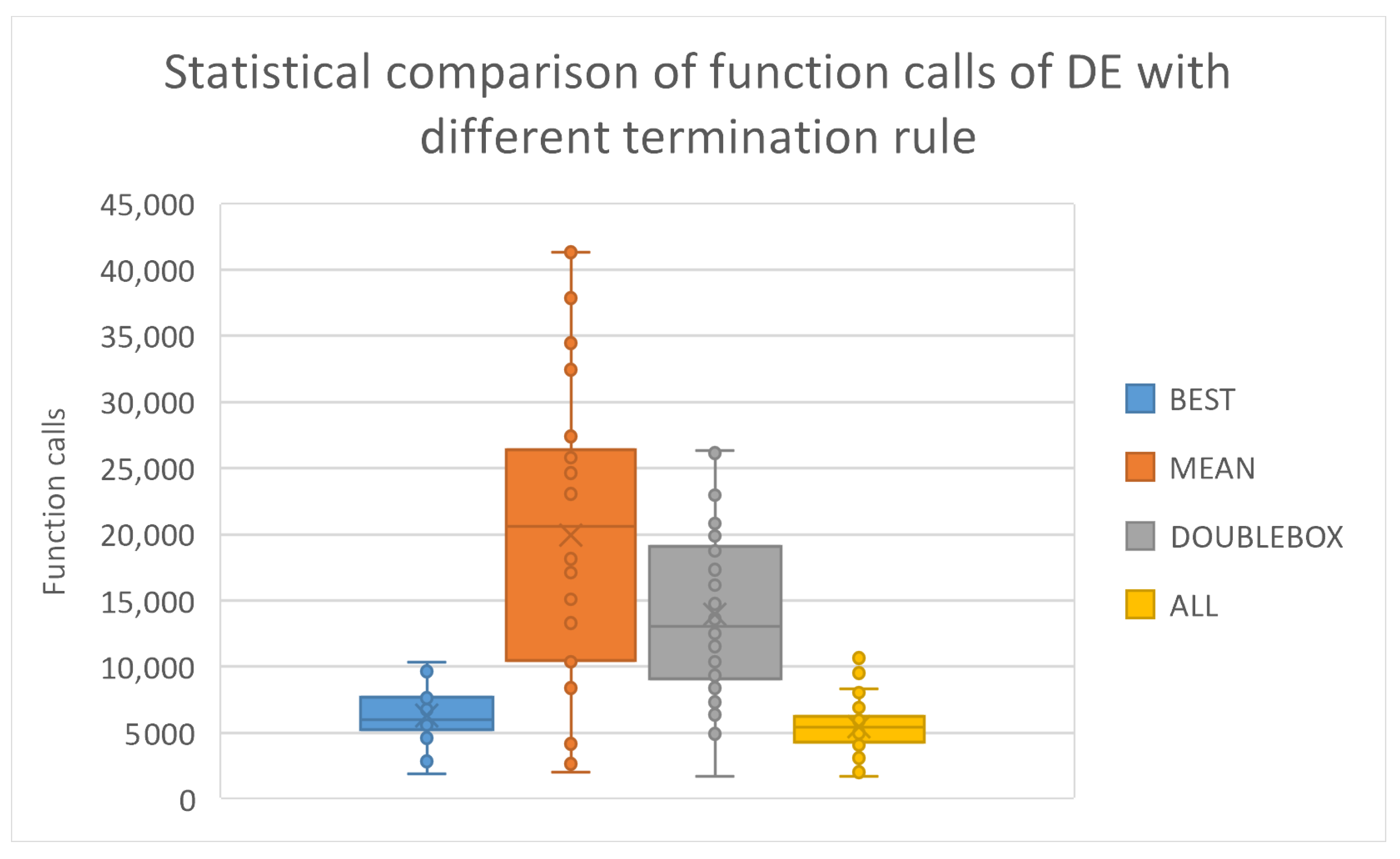
All tables presented here demonstrate the average function calls obtained for each test problem. The average function can be considered as a measure of the speed of each method, since each function has a different complexity and therefore, the average execution time would not be a good indication of the computational time required. In the first set of experiments we examined if the presence of the suggested stopping rule, which is the combination of a series of stopping rules, affects the optimization techniques without parallelization. During parallel execution, the total sum of calls is computed across all computing units nodes, ensuring efficient load distribution and resource utilization. However, the algorithm terminates at the computing unit that identifies the optimal solution, signaling the achievement of the desired convergence criterion. In Table 3, we observe the performance of all termination rules for the DE method. From these, both statistical and quantitative comparisons arise, depicted in Figure 2.
Table 3.
Average function calls for the Differential evolution method, using different termination rules.
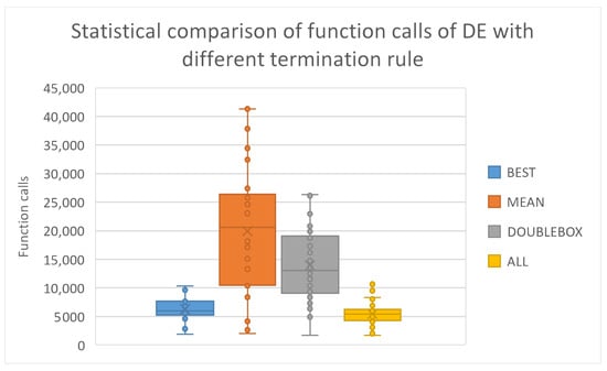
Figure 2.
Statistical comparison of function calls with different termination rules of differential evolutions.
As it is evident, the combination of the stopping rules reduces the required number of function calls that are required to obtain the global minimum by the DE method. The proposed termination scheme outperforms by a percentage that varies from 13% to 73% the other termination rules used here. In addition, in order to ascertain which of the three termination rules has the greatest effect on the termination with the mixed rule, the rule responsible for the termination of the DE optimization technique was recorded for all functions of the test set. The results from this recording are shown in Table 4. The two techniques that seem to be the most decisive for terminating each function are the Best and the DoubleBox methods, and in fact the Best method appears to significantly outperform the DoubleBox termination scheme on average.
Table 4.
Percentage of the rule which is responsible for termination in the mixed stopping rule.
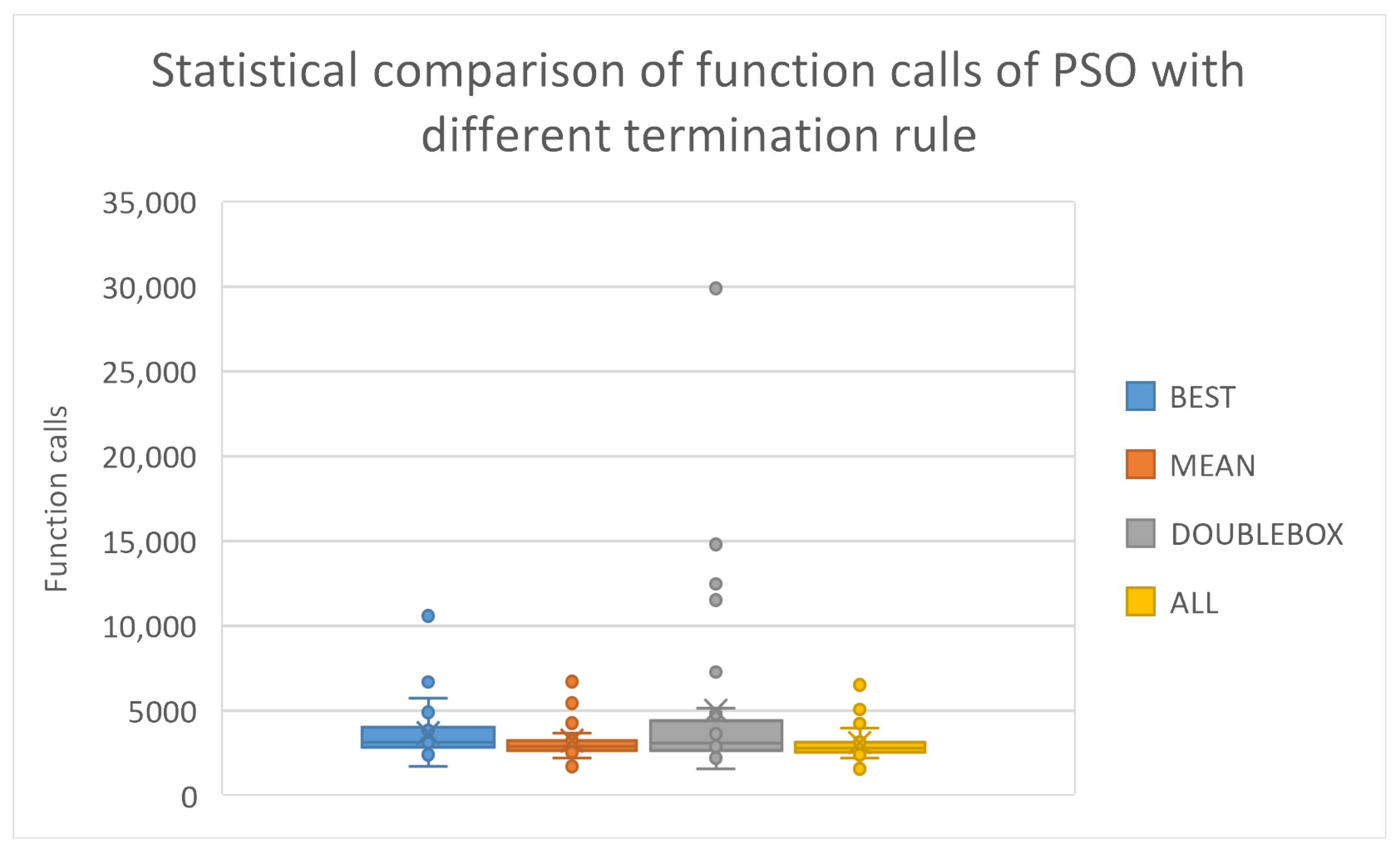
Subsequently, the same experiment was conducted for the PSO method and the results are shown in Table 5 and the statistical comparison is outlined graphically in Figure 3.
Table 5.
Average function calls for the PSO method, with different termination rules.
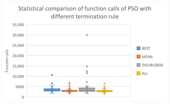
Figure 3.
Statistical comparison of function calls with different termination rule of PSO method.
Once more, the proposed termination scheme outperforms the other stopping rules in almost every test function. Likewise, the same experiment was carried out for the Multistart method and the results are depicted in Table 6 and the statistical comparison is shown in Figure 4.
Table 6.
Multistart function calls with different termination rules.
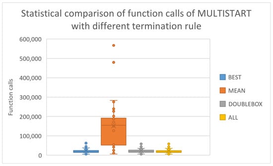
Figure 4.
Statistical comparison of function calls with different termination rule of multistart.
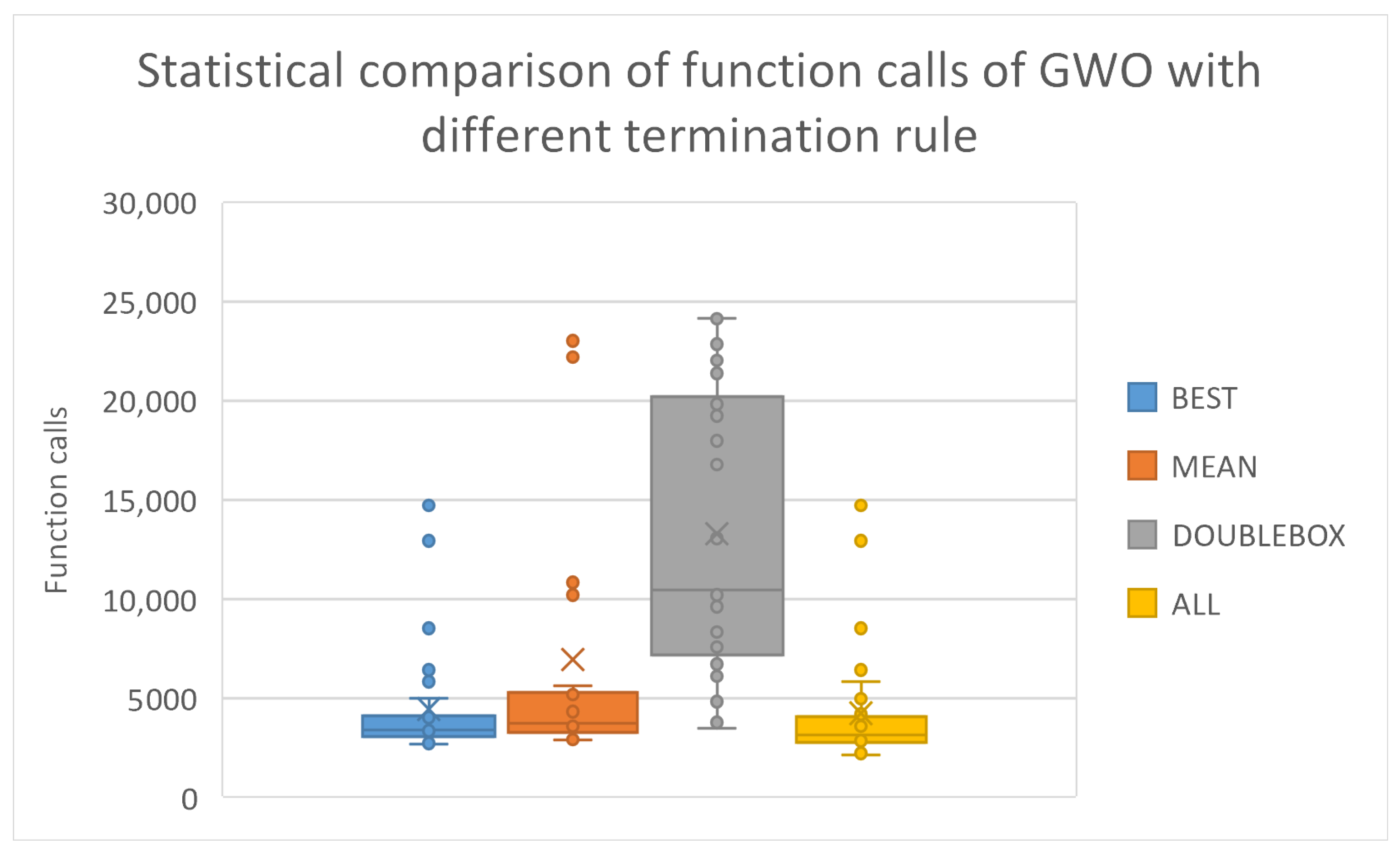
Observing the tables with the corresponding statistical and quantitative comparisons, it is evident that the calls to the objective function for the proposed termination rule are fewer than any other rule in any method. Also, the proposed termination rule was applied to a recent global optimization method named Grey Wolf Optimizer [87] and the results are shown in Table 7 and the corresponding statistical comparison in Figure 5.
Table 7.
Experiments using the variety of termination rules and the GWO optimization method.
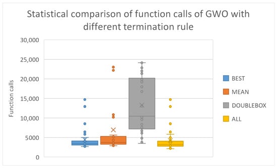
Figure 5.
Statistical comparison for the GWO optimizer using different termination rules.
Once again the combinatorial termination technique achieves the lowest number of function calls of all available techniques. Each optimization method and termination criterion function differently and yield varying results. This variation is further influenced by the differing nature of the cost functions involved. When integrated into the overall algorithm, each method, in combination with the termination criterion that best suits it, can converge to optimal solutions more quickly, thereby enhancing the algorithm’s overall performance.
The proposed termination rule was also applied to the current parallel optimization technique for the test functions described previously. The experimental results for the so-called DoubleBox stopping rule and the given parallel method are shown in Table 8. The columns in the table stand for the following:
Table 8.
Experiments using the proposed optimization technique and the DoubleBox stopping rule. The experiment was performed on the test functions described previously. Numbers in cells denote average function calls.
- Column Problem denotes the test function used.
- Column 1 × 500 denotes the application of the proposed technique with one processing unit and 500 particles.
- Column 2 × 250 stands for the usage of two processing units. In each unit, the number of particles was set to 250.
- Column 5 × 100 denotes the incorporation of 5 processing units into the proposed method. In each processing unit the number of particles was set to 100.
- Column 10 × 50 stands for the usage of 10 processing units. In each processing unit, the number of particles was set to 50.
In this experiment, the total number of particles was set to 500, in order to have credibility in the values recorded. The results indicate that the increase in processing units may reduce the required number of function calls. The same series of experiments was also conducted using the so-called mean fitness termination rule, which has been described in Equations (2) and (3). The obtained results are presented in Table 9 and Table 10.
Table 9.
Experiments using the proposed optimization technique and the mean—fitness stopping rule. Numbers in cells denote average function calls.
Table 10.
Experiments using the proposed optimization technique and the best—fitness stopping rule. Numbers in cells denote average function calls.
And, in this series of experiments, the columns of the table retain the same meaning as in Table 8. Furthermore, once again, it is observed that the increase in the number of computing units significantly reduces the required number of function calls to find the global minimum. Additionally, there is a significant reduction in the number of function calls required to be compared to the previous termination rule. Finally, the proposed termination rule is utilized in the parallel optimization technique and the experimental results are outlined in Table 11.
Table 11.
Experiments using the proposed optimization technique and proposed stopping rule. Numbers in cells denote average function calls.
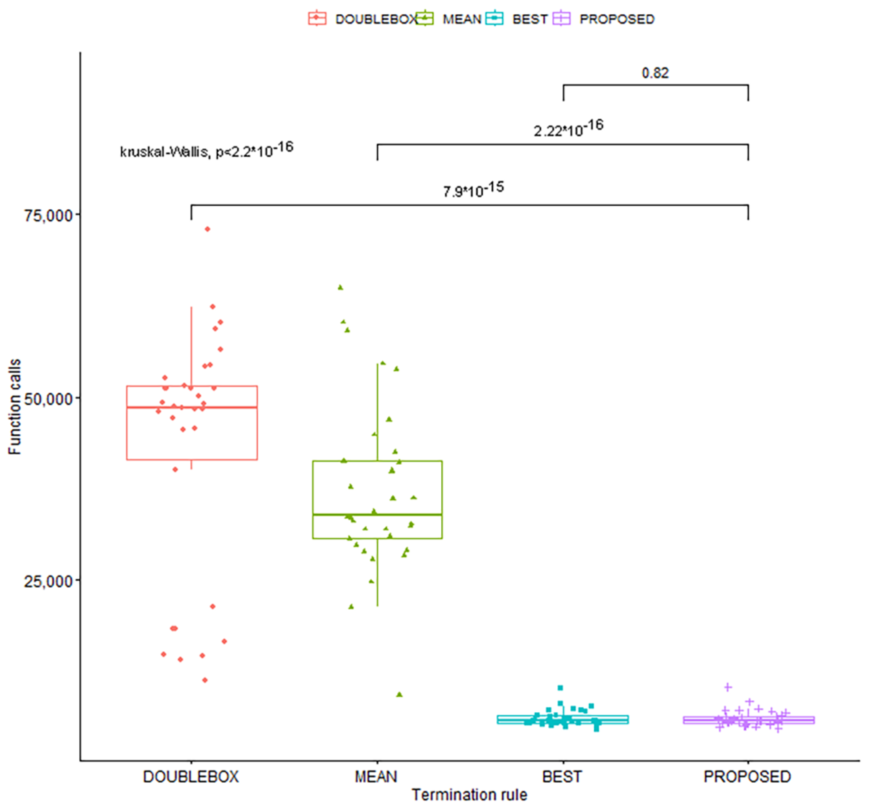
And, in this case, it is observed that the increase in parallel processing units significantly reduces the required number of function calls, as in the two previous termination rules. However, the proposed termination rule dramatically reduces the number of required function calls and consequently the computation time compared to previous termination rules. This reduction in fact intensifies as the number of computing nodes increases. Also, for the same set of experiments, a statistical test (Wilcoxon test) was conducted and it is graphically presented in Figure 6.
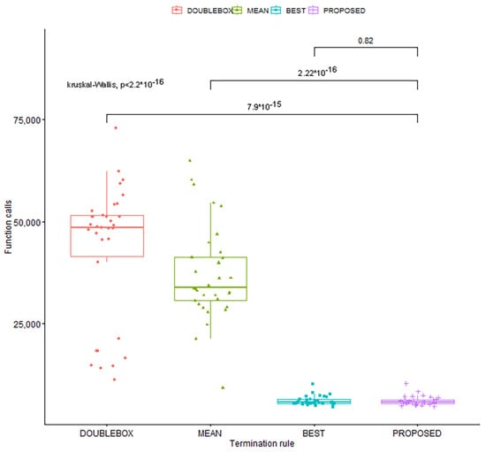
Figure 6.
Wilcoxon rank–sum test results for the comparison of different termination rules as used in the proposed parallel optimization technique and for five processing units.
A p-value of less than 0.05 (two-tailed) was used to determine statistical significance and is indicated in bold.
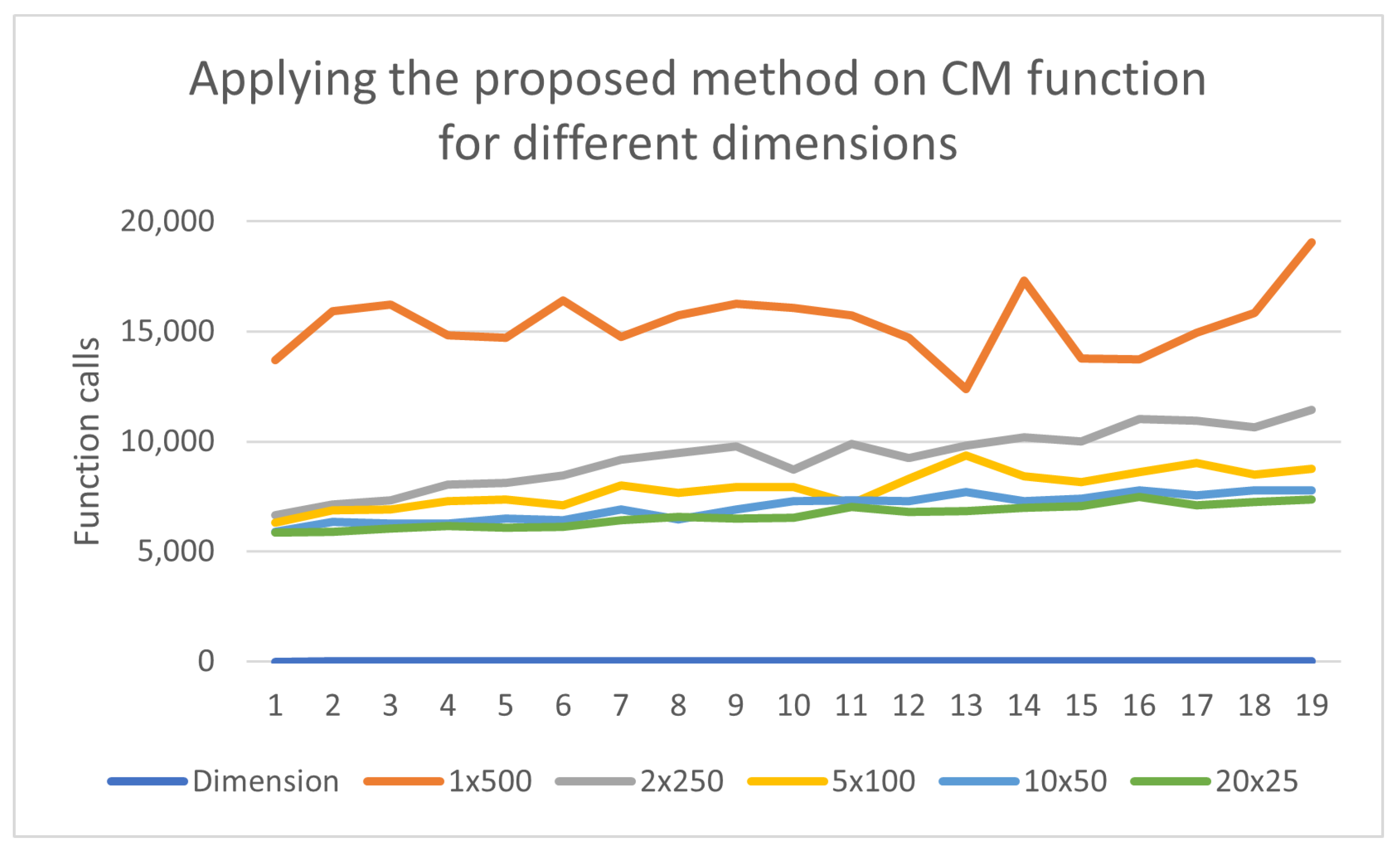
An additional experiment was performed to assess the capabilities of the parallel technique using the CM function for various values of the dimension. This function is defined as:
The proposed method was tested on this function for different values of the dimension n and for a variety of processing units and the results are graphically illustrated in Figure 7.
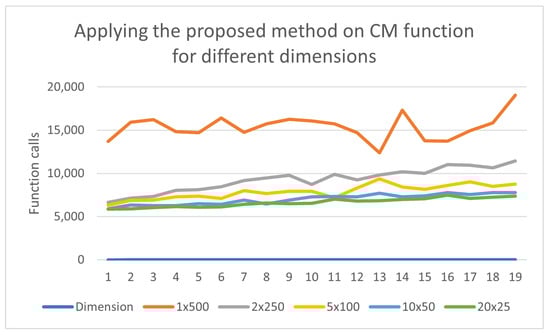
Figure 7.
Experiments using the proposed parallel technique and the CM function. The dimension of the function n varies from 1 to 20 and the number of processing units changes from 1 to 20.
From the experimental results, it is obvious that the required number of function calls is drastically reduced with the increase in computing units from 1 to 2 or to 5.
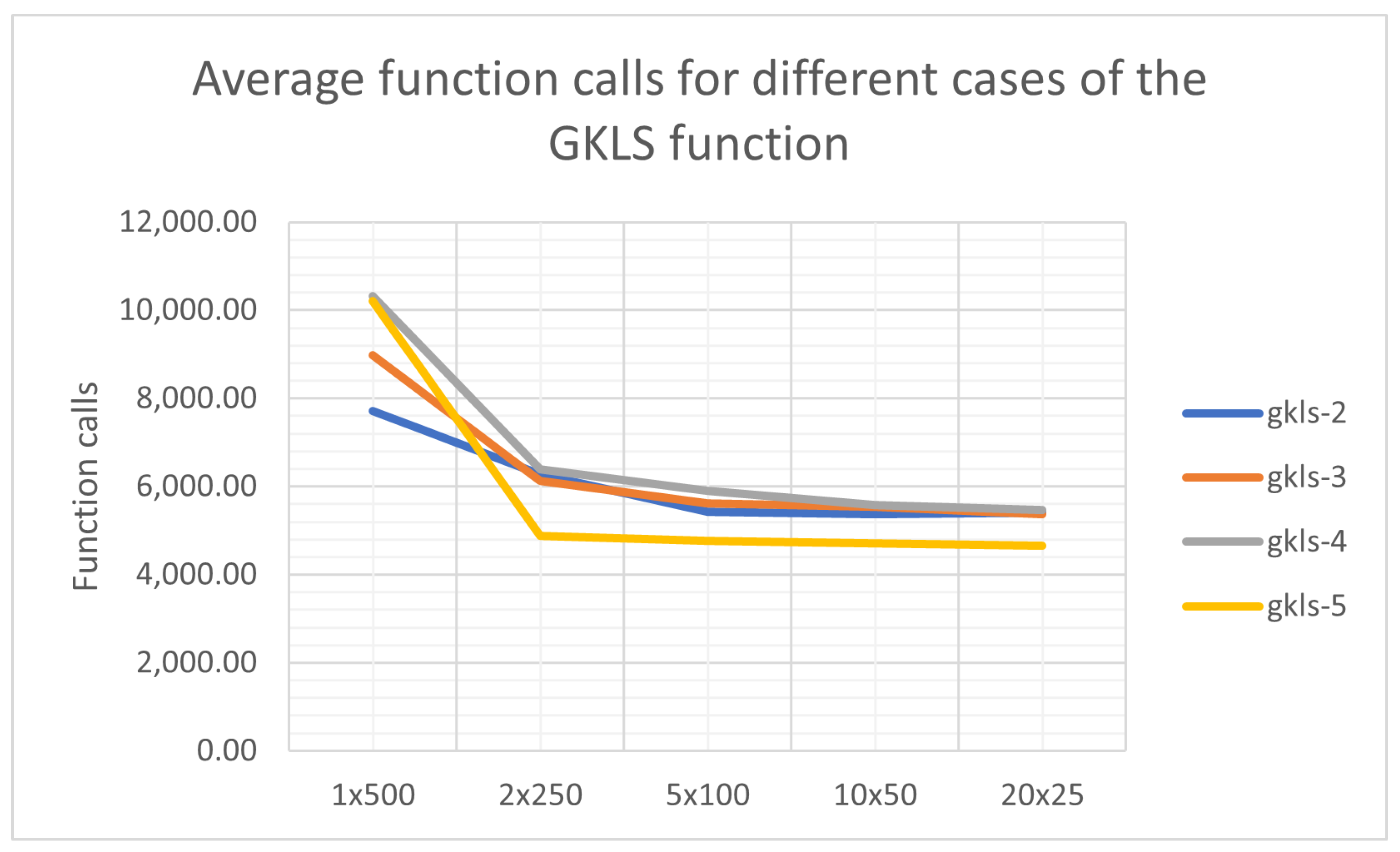
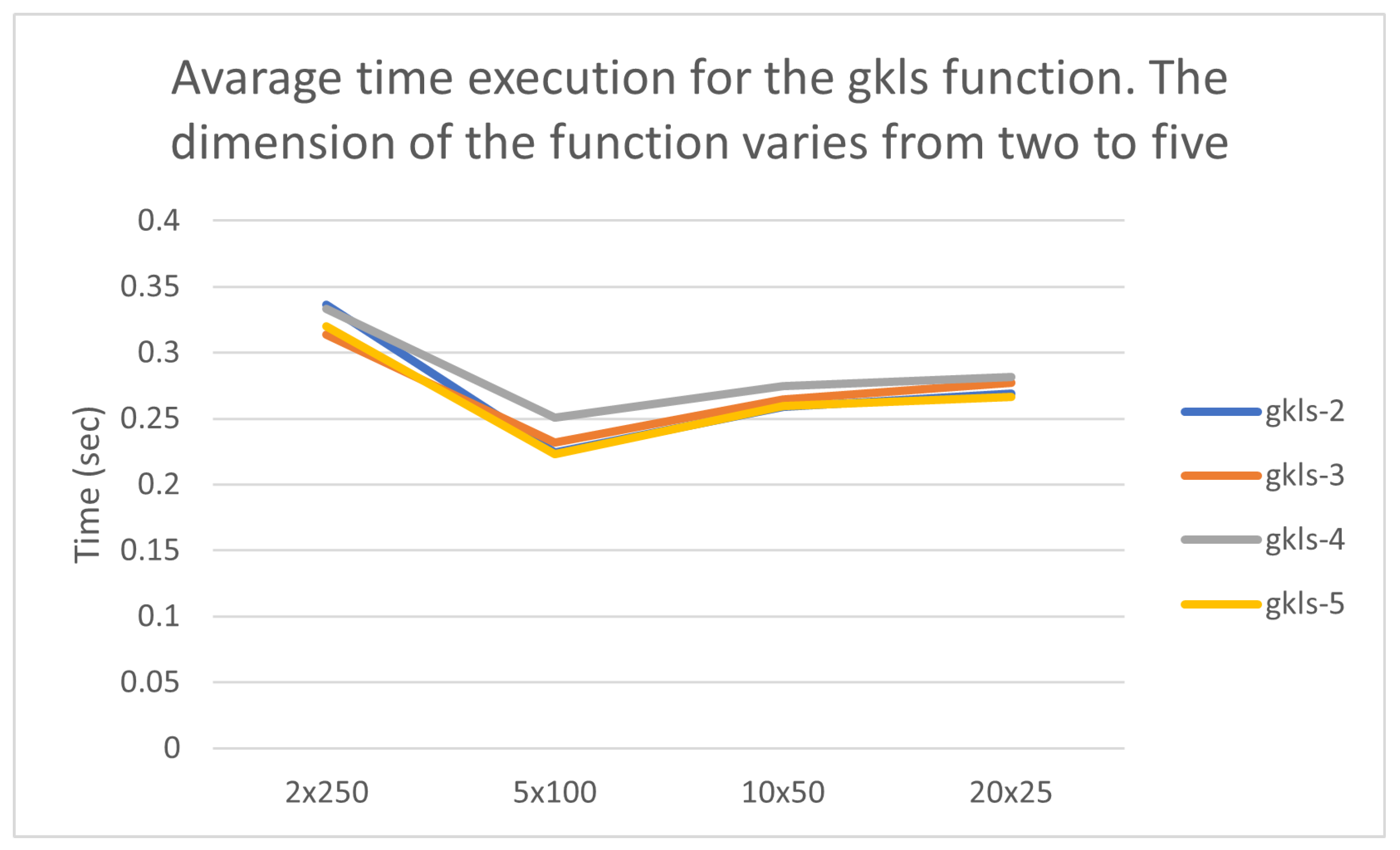
Also, the proposed method was applied on the GKLS function for different versions of the function. The dimension of the function was in the range . In each dimension, 10 different versions of the functions were used and average execution times and function calls were recorded. Also, the proposed method was applied on the GKLS function using different numbers of processing units. The average function calls from this experiment are show graphically in Figure 8 and the average execution times in Figure 9.
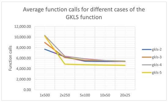
Figure 8.
Average function calls for the proposed method and different dimensions of the GKLS function.
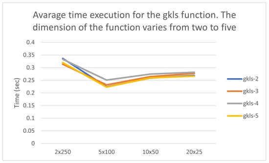
Figure 9.
Average execution time for the GKLS function and the proposed method.
The graphs above show once again that adding processing units to the proposed technique can reduce not only the execution time, as expected, but also the required number of function calls. In the specific scheme, the execution time increases slightly for a certain number of execution units and above, as this time also includes the time spent by the execution engine for the synchronization of the processing units as well as for the exchange of information between them.
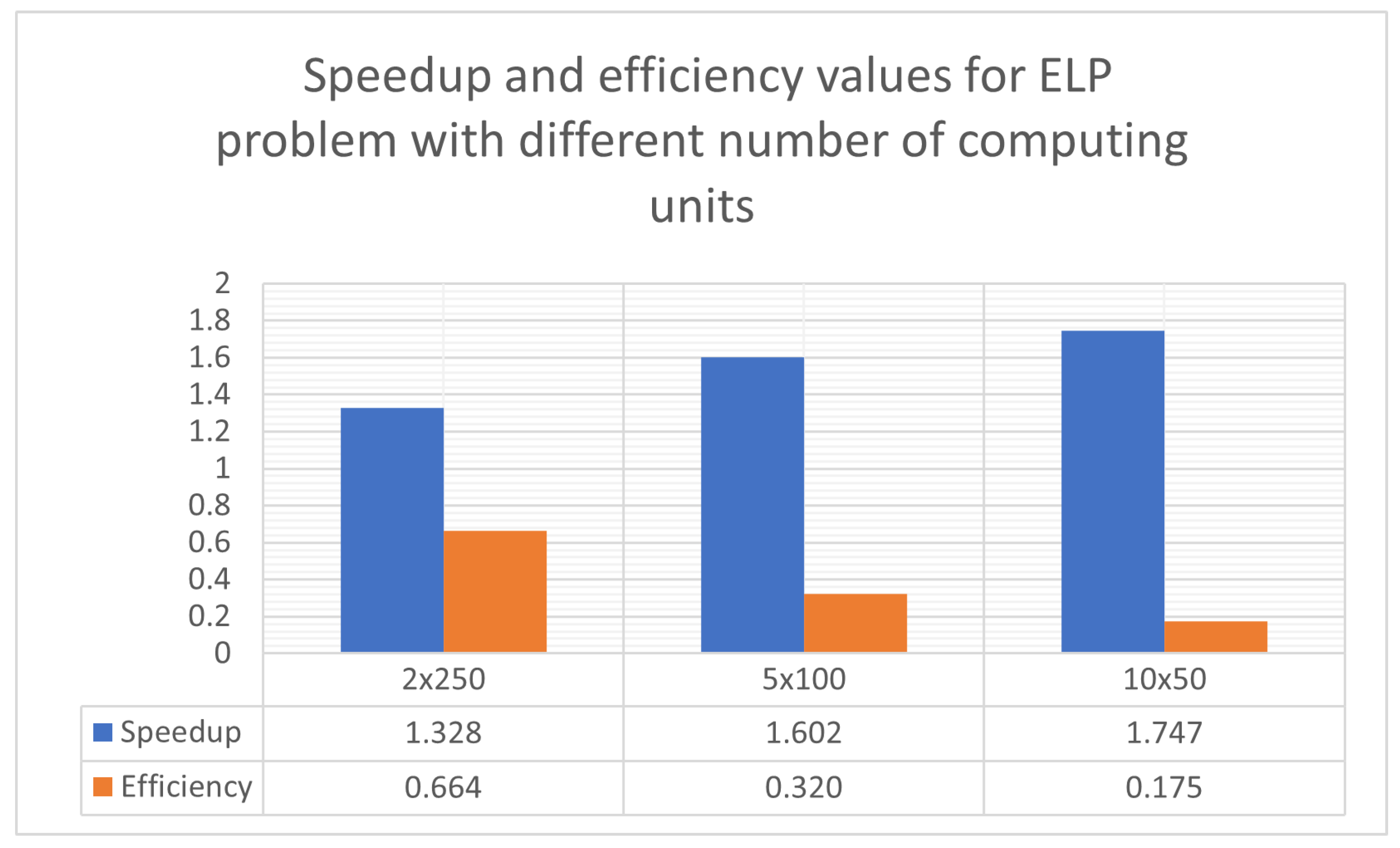
Furthermore, in Figure 10, the behavior of speedup and efficiency is depicted as a function of the number of PUs. The execution of the algorithm with a single processing unit, where the speedup is 1, serves as the reference point. As the number of PUs increases, a corresponding increase in speedup is observed, though it is often less than the ideal (equal to the number of PUs) due to communication delays and overhead. Conversely, efficiency decreases with the increase in PUs, a common phenomenon in parallel computing, caused by non-linear scaling and uneven workload distribution.

Figure 10.
Speedup and efficiency of the parallel approach.
5. Conclusions
In this paper, the use of mixed termination rules for global optimization methods was thoroughly presented, and a new global optimization method that takes full advantage of parallel computing structures was afterward proposed. The use of mixed termination rules leads a series of computational global optimization techniques to find the global minimum of the objective function faster, as was also shown by the experimental results. The termination rules exploited are based on asymptotic criteria and are general enough to be applicable to any global optimization problem and stochastic global optimization technique.
Furthermore, the new stopping rule is utilized in a novel stochastic global optimization technique that involves some basic global optimization techniques. This method is designed to be executed in parallel computation environments. At each step of the method, a different global optimization method is also executed on each parallel computing unit, and these different techniques exchange optimal solutions with each other. In current work, the global optimization techniques of Differential Evolution, Multistart and PSO were used in the processing units, but the method can be generalized to use other stochastic optimization techniques, such as genetic algorithms or simulated annealing. Also, the overall method terminates with the combined termination rule proposed here, and the experimental results performed on a series of well-known test problems from the relevant literature seem to be very promising.
However, the present work is limited to a specific set of optimization methods and termination criteria. Therefore, future extensions of this work may include the integration of additional and more advanced termination criteria, as well as the implementation of alternative global optimization methods in the processing units, such as genetic algorithms or variations of simulated annealing.
Author Contributions
V.C., I.G.T. and A.M.G. conceived the idea and methodology and supervised the technical part regarding the software. V.C. conducted the experiments. A.M.G. performed the statistical analysis. I.G.T. and all other authors prepared the manuscript. All authors have read and agreed to the published version of the manuscript.
Funding
This research received no external funding.
Institutional Review Board Statement
Not applicable.
Informed Consent Statement
Not applicable.
Data Availability Statement
Data are contained within the article.
Acknowledgments
This research has been financed by the European Union: Next Generation EU through the Program Greece 2.0 National Recovery and Resilience Plan, under the call RESEARCH—CREATE—INNOVATE, project name “iCREW: Intelligent small craft simulator for advanced crew training using Virtual Reality techniques” (project code: TAEDK-06195).
Conflicts of Interest
The authors have no conflicts of interest to declare.
References
- Honda, M. Application of genetic algorithms to modelings of fusion plasma physics. Comput. Phys. Commun. 2018, 231, 94–106. [Google Scholar] [CrossRef]
- Luo, X.L.; Feng, J.; Zhang, H.H. A genetic algorithm for astroparticle physics studies. Comput. Phys. Commun. 2020, 250, 106818. [Google Scholar] [CrossRef]
- Aljohani, T.M.; Ebrahim, A.F.; Mohammed, O. Single and Multiobjective Optimal Reactive Power Dispatch Based on Hybrid Artificial Physics–Particle Swarm Optimization. Energies 2019, 12, 2333. [Google Scholar] [CrossRef]
- Pardalos, P.M.; Shalloway, D.; Xue, G. Optimization methods for computing global minima of nonconvex potential energy functions. J. Glob. Optim. 1994, 4, 117–133. [Google Scholar] [CrossRef]
- Liwo, A.; Lee, J.; Ripoll, D.R.; Pillardy, J.; Scheraga, H.A. Protein structure prediction by global optimization of a potential energy function. Biophysics 1999, 96, 5482–5485. [Google Scholar] [CrossRef]
- An, J.; He, G.; Qin, F.; Li, R.; Huang, Z. A new framework of global sensitivity analysis for the chemical kinetic model using PSO-BPNN. Comput. Chem. Eng. 2018, 112, 154–164. [Google Scholar] [CrossRef]
- Gaing, Z.L. Particle swarm optimization to solving the economic dispatch considering the generator constraints. IEEE Trans. Power Syst. 2003, 18, 1187–1195. [Google Scholar] [CrossRef]
- Basu, M. A simulated annealing-based goal-attainment method for economic emission load dispatch of fixed head hydrothermal power systems. Int. J. Electr. Power Energy Systems 2005, 27, 147–153. [Google Scholar] [CrossRef]
- Cherruault, Y. Global optimization in biology and medicine. Math. Comput. Model. 1994, 20, 119–132. [Google Scholar] [CrossRef]
- Lee, E.K. Large-Scale Optimization-Based Classification Models in Medicine and Biology. Ann. Biomed. Eng. 2007, 35, 1095–1109. [Google Scholar] [CrossRef]
- Wolfe, M.A. Interval methods for global optimization. Appl. Math. Comput. 1996, 75, 179–206. [Google Scholar]
- Csendes, T.; Ratz, D. Subdivision Direction Selection in Interval Methods for Global Optimization. SIAM J. Numer. Anal. 1997, 34, 922–938. [Google Scholar] [CrossRef]
- Kirkpatrick, S.; Gelatt, C.D.; Vecchi, M.P. Optimization by simulated annealing. Science 1983, 220, 671–680. [Google Scholar] [CrossRef]
- Hashim, F.A.; Houssein, E.H.; Mabrouk, M.S.; Al-Atabany, W.; Mirjalili, S. Henry gas solubility optimization: A novel physics based algorithm. Future Gener. Comput. Syst. 2019, 101, 646–667. [Google Scholar] [CrossRef]
- Rashedi, E.; Nezamabadi-Pour, H.; Saryazdi, S. GSA: A gravitational search algorithm. Inf. Sci. 2009, 179, 2232–2248. [Google Scholar] [CrossRef]
- Du, H.; Wu, X.; Zhuang, J. Small-World Optimization Algorithm for Function Optimization. In Proceedings of the International Conference on Natural Computation, Xi’an, China, 24–28 September 2006; pp. 264–273. [Google Scholar] [CrossRef]
- Goldberg, D.E.; Holland, J.H. Genetic Algorithms and Machine Learning. Mach. Learn. 1988, 3, 95–99. [Google Scholar] [CrossRef]
- Das, S.; Suganthan, P.N. Differential evolution: A survey of the state-of-the-art. IEEE Trans. Evol. Comput. 2011, 15, 4–31. [Google Scholar] [CrossRef]
- Charilogis, V.; Tsoulos, I.G.; Tzallas, A.; Karvounis, E. Modifications for the Differential Evolution Algorithm. Symmetry 2022, 14, 447. [Google Scholar] [CrossRef]
- Kennedy, J.; Eberhart, R. Particle Swarm Optimization. In Proceedings of the ICNN’95—International Conference on Neural Networks, Perth, WA, Australia, 27 November–1 December 1995; Volume 4, pp. 1942–1948. [Google Scholar] [CrossRef]
- Charilogis, V.; Tsoulos, I.G. Toward an Ideal Particle Swarm Optimizer for Multidimensional Functions. Information 2022, 13, 217. [Google Scholar] [CrossRef]
- Dorigo, M.; Maniezzo, V.; Colorni, A. Ant system: Optimization by a colony of cooperating agents. IEEE Trans. Syst. Man Cybern. Part B (Cybern.) 1996, 26, 29–41. [Google Scholar] [CrossRef]
- Yang, X.S.; Gandomi, A.H. Bat algorithm: A novel approach for global engineering optimization. Eng. Comput. 2012, 29, 464–483. [Google Scholar] [CrossRef]
- Mirjalili, S.; Lewis, A. The whale optimization algorithm. Adv. Eng. Softw. 2016, 95, 51–67. [Google Scholar] [CrossRef]
- Saremi, S.; Mirjalili, S.; Lewis, A. Grasshopper optimisation algorithm: Theory and application. Adv. Eng. Softw. 2017, 105, 30–47. [Google Scholar] [CrossRef]
- Chu, S.C.; Roddick, J.F.; Pan, J.S. A parallel particle swarm optimization algorithm with communication strategies. J. Inf. Sci. Eng. 2005, 21, 809–818. [Google Scholar]
- Larson, J.; Wild, S.M. Asynchronously parallel optimization solver for finding multiple minima. Math. Program. Comput. 2018, 10, 303–332. [Google Scholar] [CrossRef]
- Tsoulos, I.G.; Tzallas, A.; Tsalikakis, D. PDoublePop: An implementation of parallel genetic algorithm for function optimization. Comput. Phys. Commun. 2016, 209, 183–189. [Google Scholar] [CrossRef]
- Kamil, R.; Reiji, S. An Efficient GPU Implementation of a Multi-Start TSP Solver for Large Problem Instances. In Proceedings of the 14th Annual Conference Companion on Genetic and Evolutionary Computation, Philadelphia, PA, USA, 7–11 July 2012; pp. 1441–1442. [Google Scholar]
- Van Luong, T.; Melab, N.; Talbi, E.G. GPU-Based Multi-start Local Search Algorithms. In Learning and Intelligent Optimization. LION 2011; Coello, C.A.C., Ed.; Lecture Notes in Computer Science; Springer: Berlin/Heidelberg, Germany, 2011; Volume 6683. [Google Scholar]
- Barkalov, K.; Gergel, V. Parallel global optimization on GPU. J. Glob. Optim. 2016, 66, 3–20. [Google Scholar] [CrossRef]
- Low, Y.; Gonzalez, J.; Kyrola, A.; Bickson, D.; Guestrin, C.; Hellerstein, J. GraphLab: A New Framework for Parallel Machine Learning. arXiv 2014, arXiv:1408.2041. [Google Scholar]
- Yangyang, L.; Liu, G.; Lu, G.; Jiao, L.; Marturi, N.; Shang, R. Hyper-Parameter Optimization Using MARS Surrogate for Machine-Learning Algorithms. IEEE Trans. Emerg. Top. Comput. 2019, 99, 1–11. [Google Scholar]
- Yamashiro, H.; Nonaka, H. Estimation of processing time using machine learning and real factory data for optimization of parallel machine scheduling problem. Oper. Res. Perspect. 2021, 8, 100196. [Google Scholar] [CrossRef]
- Kim, H.S.; Tsai, L. Design Optimization of a Cartesian Parallel Manipulator. J. Mech. Des. 2003, 125, 43–51. [Google Scholar] [CrossRef]
- Oh, S.; Jang, H.J.; Pedrycz, W. The design of a fuzzy cascade controller for ball and beam system: A study in optimization with the use of parallel genetic algorithms. ScienceDirect Eng. Artif. Intell. 2009, 22, 261–271. [Google Scholar] [CrossRef]
- Fatehi, M.; Toloei, A.; Zio, E.; Niaki, S.T.A.; Kesh, B. Robust optimization of the design of monopropellant propulsion control systems using an advanced teaching-learning-based optimization method. Eng. Appl. Artif. Intell. 2023, 126, 106778. [Google Scholar] [CrossRef]
- Cai, J.; Yang, H.; Lai, T.; Xu, K. Parallel pump and chiller system optimization method for minimizing energy consumption based on a novel multi-objective gorilla troops optimizer. J. Build. Eng. 2023, 76, 107366. [Google Scholar] [CrossRef]
- Yu, Y.; Shahabi, L. Optimal infrastructure in microgrids with diverse uncertainties based on demand response, renewable energy sources and two-stage parallel optimization algorithm. Eng. Artif. Intell. 2023, 123, 106233. [Google Scholar] [CrossRef]
- Ramirez-Gil, F.J.; Pere-Madrid, C.M.; Silva, E.C.N.; Montealerge-Rubio, W. Sustainable Parallel computing for the topology optimization method: Performance metrics and energy consumption analysis in multiphysics problems. Comput. Inform. Syst. 2021, 30, 100481. [Google Scholar]
- Tavakolan, M.; Mostafazadeh, F.; Eirdmousa, S.J.; Safari, A.; Mirzai, K. A parallel computing simulation-based multi-objective optimization framework for economic analysis of building energy retrofit: A case study in Iran. J. Build. Eng. 2022, 45, 103485. [Google Scholar] [CrossRef]
- Lin, G. Parallel Optimization n Based Operational Planning to Enhance the Resilience of Large-Scale Power Systems. Mississippi State University, Scholars Junction. 2020. Available online: https://scholarsjunction.msstate.edu/td/3436/ (accessed on 24 July 2024).
- Pang, M.; Shoemaker, C.A. Comparison of parallel optimization algorithms on computationally expensive groundwater remediation designs. Sci. Total Environ. 2023, 857, 159544. [Google Scholar] [CrossRef] [PubMed]
- Ezugwu, A. A general Framework for Utilizing Metaheuristic Optimization for Sustainable Unrelated Parallel Machine Scheduling: A concise overview. arXiv 2023, arXiv:2311.12802. [Google Scholar]
- Censor, Y.; Zenios, S. Parallel Optimization: Theory, Algorithms and Applications; Oxford University Press: Oxford, UK, 1998; ISBN 13: 978-0195100624. [Google Scholar] [CrossRef]
- Onbaşoğlu, E.; Özdamar, L. Parallel simulated annealing algorithms in global optimization. J. Glob. Optim. 2001, 19, 27–50. [Google Scholar] [CrossRef]
- Schutte, J.F.; Reinbolt, J.A.; Fregly, B.J.; Haftka, R.T.; George, A.D. Parallel global optimization with the particle swarm algorithm. Int. J. Numer. Methods Eng. 2004, 61, 2296–2315. [Google Scholar] [CrossRef] [PubMed]
- Regis, R.G.; Shoemaker, C.A. Parallel stochastic global optimization using radial basis functions. Informs J. Comput. 2009, 21, 411–426. [Google Scholar] [CrossRef]
- Gallegos Lizárraga, R.A. Parallel Computing for Real-Time Image Processing. Preprints 2024, 2024080040. [Google Scholar] [CrossRef]
- Afzal, A.; Ansari, Z.; Faizabadi, A.R.; Ramis, M. Parallelization Strategies for Computational Fluid Dynamics Software: State of the Art Review. Arch. Comput. Methods Eng. 2017, 24, 337–363. [Google Scholar] [CrossRef]
- Zou, Y.; Zhu, Y.; Li, Y.; Wu, F.X.; Wang, J. Parallel computing for genome sequence processing. Briefings Bioinform. 2021, 22, bbab070. [Google Scholar] [CrossRef] [PubMed]
- Gutiérrez, J.M.; Cofiño, A.S.; Ivanissevich, M.L. An hybrid evolutive-genetic strategy for the inverse fractal problem of IFS models. In Ibero-American Conference on Artificial Intelligence; Springer: Berlin/Heidelberg, Germany, 2000; pp. 467–476. [Google Scholar]
- Tahir, M.; Sardaraz, M.; Mehmood, Z.; Muhammad, S. CryptoGA: A cryptosystem based on genetic algorithm for cloud data security. Clust. Comput. 2021, 24, 739–752. [Google Scholar] [CrossRef]
- Lucasius, C.B.; Kateman, G. Genetic algorithms for large-scale optimization in chemometrics: An application. TrAC Trends Anal. Chem. 1991, 10, 254–261. [Google Scholar] [CrossRef]
- Sangeetha, M.; Sabari, A. Genetic optimization of hybrid clustering algorithm in mobile wireless sensor networks. Sens. Rev. 2018, 38, 526–533. [Google Scholar]
- Ghaheri, A.; Shoar, S.; Naderan, M.; Shahabuddin Hoseini, S. The Applications of Genetic Algorithms in Medicine. J. List Oman Med. J. 2015, 30, 406–416. [Google Scholar] [CrossRef] [PubMed]
- Marini, F.; Walczak, B. Particle swarm optimization (PSO). A tutorial. Chemom. Intell. Lab. Syst. 2015, 149, 153–165. [Google Scholar] [CrossRef]
- García-Gonzalo, E.; Fernández-Martínez, J.L. A Brief Historical Review of Particle Swarm Optimization (PSO). J. Bioinform. Intell. Control 2012, 1, 3–16. [Google Scholar] [CrossRef]
- Jain, M.; Saihjpal, V.; Singh, N.; Singh, S.B. An Overview of Variants and Advancements of PSO Algorithm. Appl. Sci. 2022, 12, 8392. [Google Scholar] [CrossRef]
- de Moura Meneses, A.A.; Dornellas, M.; Schirru, M.R. Particle Swarm Optimization applied to the nuclear reload problem of a Pressurized Water Reactor. Prog. Nucl. Energy 2009, 51, 319–326. [Google Scholar] [CrossRef]
- Shaw, R.; Srivastava, S. Particle swarm optimization: A new tool to invert geophysical data. Geophysics 2007, 72, F75–F83. [Google Scholar] [CrossRef]
- Ourique, C.O.; Biscaia, E.C.; Pinto, J.C. The use of particle swarm optimization for dynamical analysis in chemical processes. Comput. Chem. Eng. 2002, 26, 1783–1793. [Google Scholar] [CrossRef]
- Fang, H.; Zhou, J.; Wang, Z.; Qiu, Z.; Sun, Y.; Lin, Y.; Chen, K.; Zhou, X.; Pan, M. Hybrid method integrating machine learning and particle swarm optimization for smart chemical process operations. Front. Chem. Sci. Eng. 2022, 16, 274–287. [Google Scholar] [CrossRef]
- Wachowiak, M.P.; Smolikova, R.; Zheng, Y.; Zurada, J.M.; Elmaghraby, A.S. An approach to multimodal biomedical image registration utilizing particle swarm optimization. IEEE Trans. Evol. Comput. 2004, 8, 289–301. [Google Scholar] [CrossRef]
- Marinakis, Y.; Marinaki, M.; Dounias, G. Particle swarm optimization for pap-smear diagnosis. Expert Syst. Appl. 2008, 35, 1645–1656. [Google Scholar] [CrossRef]
- Park, J.B.; Jeong, Y.W.; Shin, J.R.; Lee, K.Y. An Improved Particle Swarm Optimization for Nonconvex Economic Dispatch Problems. IEEE Trans. Power Syst. 2010, 25, 156–166. [Google Scholar] [CrossRef]
- Feoktistov, V. Differential Evolution. In Search of Solutions. Optimization and Its Applications; Springer: Berlin/Heidelberg, Germany, 2006. [Google Scholar] [CrossRef]
- Bilal, M.P.; Zaheer, H.; Garcia-Hernandez, L.; Abraham, A. Differential Evolution: A review of more than two decades of research. Eng. Appl. Artif. Intell. 2020, 90, 103479. [Google Scholar] [CrossRef]
- Rocca, P.; Oliveri, G.; Massa, A. Differential Evolution as Applied to Electromagnetics. IEEE Antennas Propag. Mag. 2011, 53, 38–49. [Google Scholar] [CrossRef]
- Lee, W.S.; Chen, Y.T.; Kao, Y. Optimal chiller loading by differential evolution algorithm for reducing energy consumption. Energy Build. 2011, 43, 599–604. [Google Scholar] [CrossRef]
- Yuan, Y.; Xu, H. Flexible job shop scheduling using hybrid differential evolution algorithms. Comput. Ind. Eng. 2013, 65, 246–260. [Google Scholar] [CrossRef]
- Xu, L.; Jia, H.; Lang, C.; Peng, X.; Sun, K. A Novel Method for Multilevel Color Image Segmentation Based on Dragonfly Algorithm and Differential Evolution. IEEE Access 2019, 7, 19502–19538. [Google Scholar] [CrossRef]
- Marti, R.; Resende, M.G.C.; Ribeiro, C. Multi-start methods for combinatorial optimization. Eur. J. Oper. 2013, 226, 1–8. [Google Scholar] [CrossRef]
- Marti, R.; Moreno-Vega, J.; Duarte, A. Advanced Multi-start Methods. In Handbook of Metaheuristics; Springer: Boston, MA, USA, 2010; pp. 265–281. [Google Scholar]
- Tu, W.; Mayne, R.W. Studies of multi-start clustering for global optimization. Int. J. Numer. Methods In Eng. 2002, 53, 2239–2252. [Google Scholar] [CrossRef]
- Dai, Y.H. Convergence properties of the BFGS algoritm. SIAM J. Optim. 2002, 13, 693–701. [Google Scholar] [CrossRef]
- Charilogis, V.; Tsoulos, I.G. A Parallel Implementation of the Differential Evolution Method. Analytics 2023, 2, 17–30. [Google Scholar] [CrossRef]
- Tsoulos, I.G. Modifications of real code genetic algorithm for global optimization. Appl. Math. Comput. 2008, 203, 598–607. [Google Scholar] [CrossRef]
- Charilogis, V.; Tsoulos, I.G.; Tzallas, A. An Improved Parallel Particle Swarm Optimization. SN Comput. Sci. 2023, 4, 766. [Google Scholar] [CrossRef]
- Chandra, R.; Dagum, L.; Kohr, D.; Maydan, D.; McDonald, J.; Menon, R. Parallel Programming in OpenMP; Morgan Kaufmann Publishers Inc.: San Mateo, CA, USA, 2001. [Google Scholar]
- Floudas, C.A.; Pardalos, P.M.; Adjiman, C.; Esposoto, W.; Gümüs, Z.; Harding, S.; Klepeis, J.; Meyer, C.; Schweiger, C. Handbook of Test Problems in Local and Global Optimization; Kluwer Academic Publishers: Dordrecht, The Netherlands, 1999. [Google Scholar]
- Ali, M.M.; Khompatraporn, C.; Zabinsky, Z.B. A Numerical Evaluation of Several Stochastic Algorithms on Selected Continuous Global Optimization Test Problems. J. Glob. Optim. 2005, 31, 635–672. [Google Scholar] [CrossRef]
- Gao, Z.M.; Zhao, J.; Hu, Y.R.; Chen, H.F. The Challenge for the Nature—Inspired Global Optimization Algorithms: Non-Symmetric Benchmark Functions. IEEE Access 2021, 9, 106317–106339. [Google Scholar] [CrossRef]
- Gaviano, M.; Ksasov, D.E.; Lera, D.; Sergeyev, Y.D. Software for generation of classes of test functions with known local and global minima for global optimization. ACM Trans. Math. Softw. 2003, 29, 469–480. [Google Scholar] [CrossRef]
- Lennard-Jones, J.E. On the Determination of Molecular Fields. Proc. R. Soc. Lond. A 1924, 106, 463–477. [Google Scholar]
- Zabinsky, Z.B.; Graesser, D.L.; Tuttle, M.E.; Kim, G.I. Global optimization of composite laminates using improving hit and run. In Recent Advances in Global Optimization; ACM: New York, NY, USA, 1992; pp. 343–368. [Google Scholar]
- Mirjalili, S.; Mirjalili, S.M.; Lewis, A. Grey wolf optimizer. Adv. Eng. Softw. 2014, 69, 46–61. [Google Scholar] [CrossRef]

Disclaimer/Publisher’s Note: The statements, opinions and data contained in all publications are solely those of the individual author(s) and contributor(s) and not of MDPI and/or the editor(s). MDPI and/or the editor(s) disclaim responsibility for any injury to people or property resulting from any ideas, methods, instructions or products referred to in the content. |
© 2024 by the authors. Licensee MDPI, Basel, Switzerland. This article is an open access article distributed under the terms and conditions of the Creative Commons Attribution (CC BY) license (https://creativecommons.org/licenses/by/4.0/).