Abstract
Defect detection in textile manufacturing is critically hampered by the inefficiency of manual inspection and the dual constraints of deep learning (DL) approaches. Specifically, DL models suffer from poor generalization, as the rapid iteration of fabric types makes acquiring sufficient training data impractical. Furthermore, their high computational costs impede real-time industrial deployment. To address these challenges, this paper proposes a texture-adaptive fabric defect detection method. Our approach begins with a Dynamic Subspace Feature Extraction (DSFE) technique to extract spatial luminance features of the fabric. Subsequently, a Light Field Offset-Aware Reconstruction Model (LFOA) is introduced to reconstruct the luminance distribution, effectively compensating for environmental lighting variations. Finally, we develop a texture-adaptive defect detection system to identify potential defective regions, alongside a probabilistic ‘OutlierIndex’ to quantify their likelihood of being true defects. This system is engineered to rapidly adapt to new fabric types with a small number of labeled samples, demonstrating strong generalization and suitability for dynamic industrial conditions. Experimental validation confirms that our method achieves 70.74% accuracy, decisively outperforming existing models by over 30%.
1. Introduction
Fabrics, composed of textile fibers, are extensively utilized in daily life. Fabric defects, defined as surface imperfections arising during the industrial manufacturing process, are typically attributed to factors such as machinery malfunctions, yarn inconsistencies, suboptimal processing conditions, and excessive mechanical stretching [1]. Identifying these defects is a cornerstone of quality assurance in the textile industry and is crucial for safeguarding fabric integrity. Effective defect detection is essential for maintaining product standards and controlling production costs. If the detection process is inaccurate, defective fabrics might enter the market. This can damage a manufacturer’s reputation and lead to substantial financial losses [2].
Traditional fabric defect detection has primarily relied on manual visual inspection. However, this process is susceptible to limitations such as operator fatigue, subjectivity, and low efficiency [3]. These constraints render traditional approaches inadequate for meeting the high-speed and precision demands of modern textile production. Consequently, the integration of computer vision technology has emerged as a major research and industrial trend, with numerous scholars undertaking extensive research to advance the field significantly [4,5].
Automated defect detection algorithms are broadly classified into conventional and deep learning-based approaches [6]. Conventional methods leverage handcrafted features derived from spatial or frequency domains—such as statistical models, spectral analysis, and morphological filtering—to identify anomalies [7,8]. While these algorithms exhibit computational efficiency, they suffer from key limitations. Specifically, they are highly sensitive to variations in lighting and fabric texture. Furthermore, their dependence on handcrafted features constrains their robustness and generalization capabilities in complex industrial environments. Deep learning methods, particularly those using Convolutional Neural Networks (CNNs) [9], have demonstrated superior accuracy by automatically learning hierarchical features from data [10,11]. However, their effectiveness is limited by a critical weakness: a heavy dependency on vast, meticulously annotated datasets. This dependency creates a significant bottleneck for practical applications, as the process of collecting and labeling tens of thousands of images is prohibitively labor-intensive and time-consuming.
Fabric defect detection remains a critical challenge in industrial applications due to several key factors. First, fabric defects are often slender and fine-grained, allowing them to blend easily into the fabric’s natural texture. This makes them exceptionally difficult to distinguish from normal variations, which in turn renders many detection algorithms insensitive to such fine structures. Compounding this issue, the complex and variable conditions of industrial environments can interfere with effective feature extraction, thereby reducing detection accuracy. Second, the data scarcity problem is particularly acute in the textile industry. Modern manufacturing is characterized by small-batch production and rapid product turnover. This production dynamic, combined with low defect rates, makes it nearly impossible to accumulate a large and diverse dataset of defective samples for each new fabric type. Consequently, data-hungry deep learning models often fail to generalize to new product lines. This failure necessitates costly and time-consuming retraining. Finally, real-time industrial inspection typically relies on low-power embedded systems, yet the high computational demands of deep learning models hinder timely inference on such platforms [12]. Although model compression and lightweight architectures can reduce complexity, they often compromise accuracy. In cloud-based settings, latency and instability further limit real-time performance. Additionally, the opaque nature of deep models impedes interpretability and explainability in defect classification [13].
This paper proposes a data-efficient fabric defect detection method to address the critical challenges of data scarcity, performance robustness, and deployment limitations. Our main contributions include:
- A Dynamic Subspace Feature Extraction (DSFE) method to extract global features from fabric images. DSFE is designed to capture key information along the primary directions of the fabric’s weave, which aligns well with the structural characteristics of fabric defects.
- A Light Field Offset-Aware Reconstruction Model (LFOA) to reconstruct the luminance distribution, which effectively mitigates the non-uniformity introduced by environmental lighting inconsistencies.
- A computationally efficient, texture-adaptive defect detection system. This system introduces a probabilistic ‘Outlier Index’ to characterize defects and features an embedded optimization model to autonomously tune its parameters, ensuring rapid generalization and suitability for real-time deployment.
2. Related Works
Driven by advances in computer vision, object detection has become a key task in artificial intelligence [14]. The goal of image defect detection is to automatically identify defect locations through computer algorithms. Currently, improvements in defect detection technologies primarily focus on enhancing model performance by incorporating auxiliary information, such as image content and annotation labels. Nevertheless, several key challenges persist, including effective feature integration, similarity measurement, multimodal discrepancies, and label imbalance [15].
In the field of feature extraction research, a variety of methods have made innovative breakthroughs from different directions. Khan Umer Ali proposed the Descriptor-Second-order Local Tetra-pattern (LTAP), which combines RGB color features with genetic algorithm-based feature selection and an SVM optimized by a genetic algorithm (GA) to achieve efficient classification of natural images [16]. J. Yang combined covariance matrices with SIFT to enhance scene classification performance [17]. T. Zhu improved wireless capsule endoscope image classification by reorganizing codebooks learned through Locality-constrained Linear Coding (LLC), thereby better representing private features [18]. J. Yu simplified and parallelized the SURF algorithm using FPGA to meet the real-time processing demands of large-scale spatial targets [19]. P. Maharjan proposed the “Fast LoG” method to accelerate Gaussian operations in SIFT, reducing computational complexity [20]. In the medical imaging domain, S. Gavkare utilized HOG features combined with XGBoost to achieve efficient brain tumor recognition in MRI images [21]. These methods are centered around solving domain-specific problems, optimizing feature extraction through algorithmic improvements or technological fusion. The application scenarios cover natural images, medical imaging, and spatial targets, with technical implementation and evaluation metrics varying according to domain requirements. For example, the medical field emphasizes classification accuracy, while spatial targets prioritize computational efficiency and real-time processing.
In the field of object detection, methods can generally be divided into deep learning-based approaches and traditional methods. Inspired by the successful application of deep convolutional neural networks (DCNN) in the industrial sector, researchers have begun exploring the use of deep learning algorithms for detecting fabric surface defects. In 2016, Liu et al. introduced the Single Shot MultiBox Detector (SSD) [22], which uses Convolutional Neural Networks (CNNs) as the backbone for feature extraction. By utilizing multi-layered feature maps of different scales, the SSD predicts object classes and bounding box offsets through anchor boxes, followed by non-maximum suppression for precise defect localization. Tan and Le’s EfficientDet [23] introduced a compound scaling method that increases network depth, width, and resolution while maintaining computational efficiency. This design achieves state-of-the-art object detection results while reducing computational complexity, making it highly suitable for resource-constrained applications. One of the significant breakthroughs in deep learning is the YOLO framework. Developed by Joseph Redmon, the YOLO framework revolutionized real-time object detection by introducing a grid-based approach to predict both bounding boxes and class probabilities simultaneously [24]. This pioneering single-stage object detection algorithm has greatly enhanced the efficiency of the detection process.
Neural networks have proven effective for object detection across various domains. However, applying these deep learning methods to fabric defect detection requires a large dataset of high-quality training samples. Acquiring such data is often a significant challenge.
In traditional defect detection algorithms, various methods have their own unique characteristics. Liu [25] proposed an algorithm based on multi-channel feature extraction and joint low-rank decomposition. This approach first simulates biological vision to extract robust multi-channel features, then applies joint low-rank decomposition to process the feature matrix, and finally uses threshold segmentation to locate the defect areas. This method is suitable for fabrics with complex textures and multiple types of defects. Guan [26] introduced a dynamic hierarchical detection method that simulates the human visual system in the HSV color space. By enhancing the saliency of defects through a data-driven approach, this method uses task-driven factors to define detection regions and set hierarchical thresholds for detecting different types of defects. Zhang [27] proposed an approach based on frequency domain filtering and similarity measurement, first separating fabric patterns from yarn textures and segmenting the pattern’s periodic units, followed by automatic defect detection in color-woven fabrics based on similarity measures.
3. Methods
The fundamental principle of this work is that fabric defects manifest as localized disruptions to the inherent periodicity and textural regularity of the textile weave. Based on this insight, our method is designed to first model this expected regularity and then precisely identify and characterize anomalous deviations. The specific workflow is outlined below.
The proposed method, illustrated in Figure 1, systematically implements this principle through three key stages. First, a Dynamic Subspace Feature Extraction (DSFE) method is employed to capture the key textural and structural features from the fabric images. Second, to mitigate the influence of environmental variations, a Light Field Offset-Aware (LFOA) module is then used to correct for visual inconsistencies. Finally, a texture-adaptive defect system analyzes the corrected features to quantify potential defects. This is achieved by initially using Locally Weighted Regression (LOWESS) to localize luminance outliers. A multidimensional analysis is then performed on these outliers, integrating both saliency and dispersion metrics to form a comprehensive, probabilistic OutlierIndex. Crucially, this stage is made adaptive by an embedded optimization model, which automatically tunes the outlier scaling factor —a critical parameter in the detection process—a mechanism that allows for automatic adaptation to different fabric textures during defect detection.
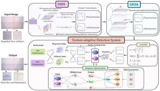
Figure 1.
Detection System Diagram.
3.1. Spatial-Domain Luminance Feature Extraction of Fabric
Fabric defects are typically slender and narrow. This characteristic makes many existing feature extraction methods insensitive to such fine structures. In contrast to prior work, this study focuses on the brightness characteristics of fabric defects. We specifically analyze how defective regions disrupt the periodicity of the spatial brightness.
The acquired textile images are converted to the HSV color space, and the V channel is extracted as the brightness feature. This study proposes a Dynamic Subspace Feature Extraction (DSFE) method, where the brightness values within each subspace are summed and averaged to obtain the V feature value of that subspace. By traversing these subspaces across the fabric image, a complete V feature sequence for the entire fabric is generated. The DSFE visualization process is shown in Figure 2.
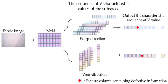
Figure 2.
Dynamic Subspace Feature Extraction Method.
Let the image brightness be denoted as , where represents the number of rows and the number of columns. For the j-th subspace, , define a subspace of size . For the x-th column, the brightness value of the sub-column space is obtained by averaging the summed brightness values within the sub-regions contained in this column, as shown in Equation (1).
The sub-column space slides along the longitudinal direction to generate the V feature sequence corresponding to the warp-direction (the lengthwise threads of the fabric) of the image, as shown in Equation (2).
Similarly, when extracting fabric information along the latitudinal direction, the subspace size is defined as , and the sub-row space dynamically covers the image along the weft direction to obtain the weft-direction (the crosswise threads) V feature sequence.
Processing near image boundaries can generate anomalous data as the subspace crosses the edge. While padding the edges with fixed values is a common approach, it can compromise feature integrity and introduce analytical bias. Therefore, our method preserves data validity by discarding data from the outermost edge regions.
This approach does not lead to a loss of critical defect information for two reasons. First, the discarded region is minimal. Its width is less than that of the sub-column space. Second, the images are captured by an array camera system that ensures significant overlap between consecutive frames. This overlapping area is substantially larger than the discarded edge region. Consequently, any defect located on the discarded edge of one image will appear in a non-edge area of the subsequent image, ensuring it is available for detection and analysis.
3.2. Reconstruction of Fabric Luminance Distribution
The distance between the overhead light source and the fabric varies from the center to the edges. This variation causes significant differences in brightness attenuation, resulting in non-uniform illumination. The backlight, used here as an auxiliary source, has a uniform intensity distribution. Therefore, it does not interfere with the fabric’s brightness distribution. In contrast, the overhead light source is fixed in position during image capture. Besides distance-related attenuation from the fixed overhead light source, ambient lighting conditions also affect the captured image. The industrial environment introduces extraneous ambient light. This ambient light combines with the fixed overhead source, disrupting the original light field balance. This disruption causes a shift in the overall light field, further contributing to uneven brightness across the image.
To mitigate the effects of environmental lighting, this study proposed a Light Field Offset-Aware Reconstruction Model (LFOA) to reconstruct the luminance distribution. Specifically, the model integrates both environmental and overhead light sources into a unified light field. This process couples them to a single, equivalent light field center.
Let the luminance of the overhead light source be P1, and that of the equivalent environmental light source be P2. The center of the fabric is designated as , and its distance to the overhead light is . For any given point on the fabric, its distance to center is . The distance between the overhead light and the equivalent environmental light is . The distance from this point to the final, unified light source is denoted by .
The distances d and L are significantly greater than the coordinates of the fabric center. Therefore, the governing equation can be simplified as follows:
Through this method, the coordinates of a single, equivalent light field center can be determined. The derivation, detailed in Equations (3)–(6), validates the feasibility of coupling the environmental and overhead light sources into a unified light field.
The combined illumination is simulated by shifting the light field’s center coordinates within the same plane. The model then calculates the distance from each fabric pixel to this center. Based on light attenuation formula, corresponding brightness compensation value is calculated for each pixel. This model effectively eliminates the combined influence of illumination during fabric image acquisition, thereby reconstructing the distribution matrix of the V feature values (Figure 3).
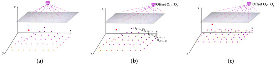
Figure 3.
Schematic diagram of LFOA, darker colors indicate higher brightness values. (a) Schematic diagram of brightness distribution with only top light source illumination; (b) Schematic diagram of unified light field and compensation; (c) Schematic diagram of the reconstructed brightness distribution.
Let denote the brightness of the light; represent the total brightness of the light source; represent the distance from the light source to the center point of the fabric, and be the actual distance from the light source to the fabric. Since the brightness at the fabric center and the distance are known, the brightness of the light source can be determined (Equation (3)). Through Equations (7) and (8), the skewness of the data calculated, and the offset distance is determined using Equations (9) and (10). Similarly, the same applies to the y-direction. By adding these offsets to the pixel coordinates, we calculate the distance from the pixel to the center of the light source.
Given the known brightness of the light source, the theoretical brightness reaching the fabric is calculated using Equations (11)–(14). Light attenuation is then determined by subtracting this theoretical brightness from the source brightness (Equation (15)). Finally, the corrected brightness value is obtained by adding times the attenuation to the measured brightness, as shown in Equation (16).
3.3. Fabric Texture-Adaptive Defect Detection System
Analysis of the reconstructed brightness distribution shows that disturbance patterns from defects differ significantly from those caused by interfering factors like wrinkles and stains [28,29,30]. Defects typically cause abrupt and transient disruptions to the periodic brightness [31]. Based on this observation, we propose a texture-adaptive defect detection method. Specifically, LOWESS is used to fit the raw brightness data. The resulting residuals are then analyzed to capture defect-related deviations. A multidimensional analysis is then conducted to represent periodic brightness anomalies. This process allows each detected defect to be graded and assigned a likelihood of being genuine. This approach effectively suppresses interference from non-defect factors.
3.3.1. Localization of Potential Defects
In some fabric images, the brightness distribution is highly scattered. Consequently, Light Field Correction alone is insufficient for effective feature extraction. To address this issue, we use LOWESS to compute a fitted curve for the V feature values. The fitting effect is shown in Figure 4a. The formula for LOWESS is as Equations (17)–(20).
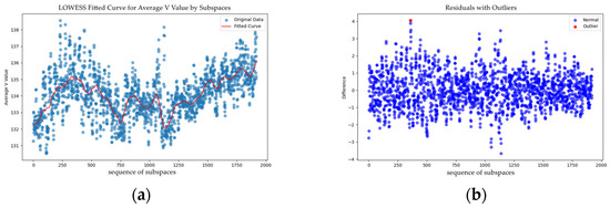
Figure 4.
(a) LOWESS Fitted Curve for Average V feature values by Subspaces; (b) Residual graph obtained after fitting.
The residual between the original V feature values and the fitted data is then calculated. For each fabric image, we calculate the mean residual value . This mean serves as the reference center for the V feature value distribution (Figure 4a). This value is then weighted with an outlier scaling factor to create an outlier discrimination coefficient. This coefficient is used to identify outliers within the dataset. Figure 4b shows the residual graph after fitting. The red dots in the figure represent the detected outliers. This LOWESS-based process effectively mitigates the influence of wrinkles, stains, and similar factors. As a result, the method achieves higher sensitivity to fabric defects and can precisely capture their subtle brightness variations.
Fabric defects are often elongated. Therefore, a small step size is used during dynamic subspace coverage to capture more detailed information. This approach ensures comprehensive data acquisition. However, it can also cause a single defect to be covered by multiple subspaces. This process generates similar outlier values in neighboring regions, creating outlier redundancy. To address this issue, this study proposes a Nearby Non-Maximum Suppression (NNMS) technique. NNMS ensures that each detected outlier is the most prominent value in its local neighborhood. This process effectively reduces redundancy.
3.3.2. Multidimensional Analytical Representation of Potential Defects
Our analysis targets periodic disturbances in the fabric’s spatial brightness. This process often identifies multiple outliers in the feature residual map. However, these outliers do not have equal significance, as their probability of representing a true defect varies considerably. To accurately assess the confidence that an outlier corresponds to a true fabric defect, this study proposes a confidence evaluation metric—OutlierIndex. This metric quantifies the association between an outlier and a genuine defect.
The OutlierIndex is evaluated comprehensively from two dimensions:
First, First, we assess the dispersion of residual data to characterize the outlier distribution. To ensure consistency, the residuals are first normalized to a unified scale. This process eliminates differences in units and magnitudes. It also reduces statistical bias caused by variations in the original data range. After normalization, the variance is computed to quantify dispersion. This standardized approach ensures that the variance reliably reflects the underlying distribution of the residuals.
The variance of the residuals is calculated according to the following Equations (21) and (22),
In Equation (23), is set to 100, denotes the maximum value of the function 0.9. and represents the center point of the curve, taken as 0.0305 in this context.
Equation (24) scales the variance to the range [0, 1].
Based on the linear distance of each outlier, a distinct dispersion weight is assigned to each outlier’s . The final , obtained through weighting, reflects the degree of data dispersion (Equations (25) and (26)).
Second, OutlierIndex is evaluated based on the magnitude of residual values. For this evaluation, we propose an improved SoftMax function. It incorporates each outlier’s residual value along with a mean adjustment factor and an outlier scaling factor derived from the residual dataset. This formulation yields a difference score for each outlier. The score is then normalized using a standard procedure.
When takes on excessively large values, the ratio decays exponentially. Under these conditions, the also decays exponentially to zero (Equations (27) and (28)). Empirical analysis shows that the discrete scaling factor rarely attains excessively large values, and there is typically a significant order-of-magnitude difference between the top value and the average value. As a result, the confidence outcomes follow a truncated normal distribution within the interval [0.5, 1]. To ensure statistical robustness, we adopt an asymmetric truncation strategy. Any calculated score below the 0.5 lower bound is mapped to this baseline value. This approach ensures both numerical stability and consistent score interpretation.
The and the are combined proportionally to form the OutlierIndex evaluation metric (Equation (29)). By introducing OutlierIndex, each outlier is assigned a corresponding confidence score. This score highlights the differences in significance and reliability among them.
3.3.3. Adaptive Optimization of the Outlier Scaling Factor
The outlier scaling factor is a critical parameter in the outlier filtering stage. Its value significantly affects performance. A high scaling factor may cause subtle defects to be overlooked. This can result in missed detections of texture anomalies. Conversely, a low scaling factor risks misclassifying noise as defects. This misclassification hinders the subsequent identification of true defects.
To address this issue, we introduce an adaptive optimization model based on a back-propagation mechanism. This model dynamically and accurately updates the outlier scaling factor during computation. This approach optimizes the outlier filtering process, thereby improving the accuracy and reliability of fabric defect detection, as illustrated in Figure 5.
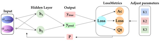
Figure 5.
Adaptive Optimization Flowchart.
In the optimization network constructed in this study, the discrete scaling factors in the warp and weft directions, denoted as an , respectively, are selected as key input parameters. The process begins with the initialization of these scaling factors, followed by forward propagation to obtain predicted outputs . These predictions are then compared with the ground truth to calculate the prediction loss. To optimize model performance, we define an adjustment factor . It is the product of the loss and term, reflecting the current change in loss, The value of is specified manually based on task requirements. Additionally, an accumulator is introduced to aggregate historical loss values. Parameter primarily controls the perception rate, which determines the parameter update step size. A larger results in faster parameter updates. Parameter regulates the granularity of observing loss changes. Smaller values allow for a more detailed analysis of loss fluctuations. Parameter defines the time span for accumulating historical losses. A higher K3 value means a richer set of past data is considered. These three parameters can be flexibly adjusted according to the specific requirements of the application scenario.
Based on the parameters , , and , combined with the real-time loss, loss change rate , and accumulated historical loss , the scaling factor deviation is calculated. This deviation , is then used to optimize the outlier scaling factor via a backpropagation algorithm. This process enhancing the overall accuracy and stability of the model (Equations (30)–(32)).
To ensure both effectiveness and efficiency, this study defines strict termination criteria for the iterative training process. Training is halted under two conditions. First, it stops if the loss function’s reduction remains below a threshold for N consecutive training rounds. Second, the process terminates when the number of training epochs reaches the preset maximum T. At this stage, the adaptive optimization model is capable of training the optimal outlier scaling coefficients for both the warp and weft directions, This provides a robust foundation for subsequent outlier filtering and fabric defect analysis. The model can thus achieve texture self-adaptation during detection, which enhances its generalization capabilities.
4. Results
This study utilized the ZD001 dataset [32], which was acquired using a high-fidelity imaging system. The system features an adaptable camera array. Images are captured with a deliberate overlap to ensure informational integrity at the edges. An alternating lighting strategy, employing both surface and backlights, was used to enhance image quality. The acquisition geometry was standardized with a lens-to-fabric distance of 82 cm and a sensor pixel size of 3.45 μm × 3.45 μm. This setup produced a final image resolution of 1920 × 1080 pixels. The data annotation was performed on-site. When testers identified a defect, they stopped the inspection machine, marked the defect on a digital device, and added a note specifying its category.
We selected a subset of 8795 images from the dataset. This subset encompasses five distinct defect types. These include three types of warp-direction defects: Broken End, Misdraw, and Reediness; and two types of weft-direction defects: Thick Place and Thin Place (Figure 6). The data distribution is presented in the following Table 1:
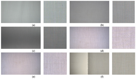
Figure 6.
The figure presents images of several common defects and their corresponding magnified views: (a) BrokenEnd; (b) Misdraw; (c) Reediness; (d) ThickPlace; (e) ThinPlace; (f) Defect images containing both fabric and background.

Table 1.
The table lists the quantities of each defect type in the dataset.
4.1. Feature Extraction Method
Methods for extracting fabric features are diverse and can be broadly categorized into four main types.
First, edge detection techniques, such as Canny and Sobel operators, capture significant pixel intensity changes by calculating image gradients. Second, feature point detection and description methods, such as Scale-Invariant Feature Transform (SIFT), identify key points within an image and generate descriptors that provide detailed representations of these points. Third, texture extraction methods, including Local Binary Patterns (LBP) and Completed LBP (CLBP), encode local grayscale variations to characterize texture. Fourth, shape and object descriptors, such as Histogram of Oriented Gradients (HOG), analyze gradient orientation distributions to describe object shapes, excelling in recognition tasks. Figure 7 illustrates the results of different feature extraction methods.
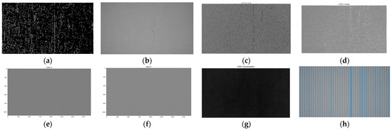
Figure 7.
The figure illustrates the results of different feature extraction methods. (a) Canny; (b) SIFT; (c) LBP; (d) CLBP; (e) Sobel X operators; (f) Sobel Y operators; (g) HOG; (h) DSFE (ours).
Fabrics are woven from yarns. Defects result from the improper positioning of these yarns and typically manifest as elongated, strip-like shapes. The extracted features from existing methods generally fall into two categories. The first includes feature point detection and texture extraction techniques, which localize defects by capturing detailed local variations. However, these methods are sensitive to interferences such as wrinkles, which also produce significant local changes. The second category comprises edge detection and shape descriptors that extract global features and filter noise. Due to the elongated nature of fabric defects, these methods risk smoothing out critical defect details. This can result in missed detections.
Therefore, effective fabric defect detection requires a balance between these two approaches. The goal is to minimize non-defect interference while accurately identifying subtle defect features. Our study addresses this by extracting continuous information from dynamic spatial subspaces. This process converts two-dimensional fabric data into continuous one-dimensional features, preserving data continuity. Brightness features from these dynamic subspaces preserve the periodic variations in the fabric. This method also allows for adaptive adjustment of the local receptive field via the subspace range. Our method detects disruptions in brightness periodicity caused by defects. It effectively suppresses non-defect interference while retaining critical defect features. By combining local detail with global structure, our method enhances detection reliability. It also provides new insights into fabric structure and imperfections.
4.2. Light Field Correction
To validate our light field correction approach, we conducted a two-part experiment. First, we addressed the issue of brightness attenuation caused by a single overhead light source. The brightness distribution from an actual fabric image is shown in Figure 8a. This distribution closely matches the theoretical attenuation curve derived from the light formula (Figure 8b). Applying our proposed LFOA formula effectively calibrates the image. This process resulting in a uniform and corrected brightness distribution as shown in Figure 8c. This result confirms the model’s efficacy for idealized single-source conditions.
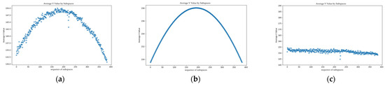
Figure 8.
(a) Original Brightness Distribution Curve; (b) Theoretical Brightness Distribution Curve; (c) Compensated Brightness Curve.
However, practical industrial environments involve not only an overhead source but also ambient light. This combination creates a more complex composite light field (Figure 9a). For comparison, Figure 9b depicts the theoretical brightness distribution that only accounts for single-source light attenuation. When a conventional correction method designed only for a single source is applied, it fails to account for the ambient component, leaving significant residual distortion in the corrected image (Figure 9c). In contrast, our comprehensive approach successfully models and eliminates the effects of both lighting components. As demonstrated in Figure 9d, the final calibrated result is a clean, interference-free brightness distribution. This result proves the model’s robustness and superiority for real-world applications.
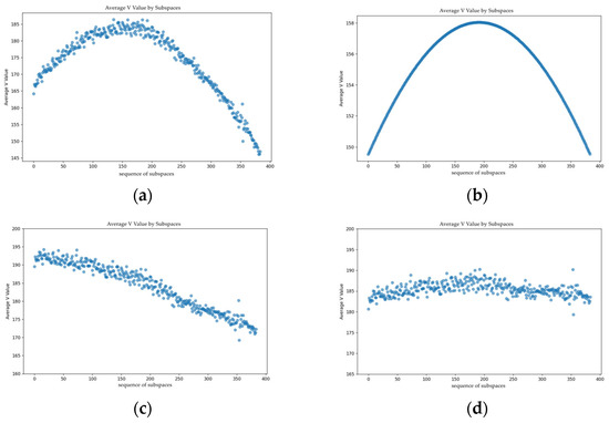
Figure 9.
(a) Original Brightness Distribution Curve; (b) Theoretical Brightness Distribution Curve; (c) Compensation Applied Only for Natural Illumination; (d) Compensation Including the Effect of Ambient Light.
4.3. Fitting Method
We evaluated various fitting methods to characterize the spatial brightness distribution of fabric images. Since the brightness distribution is not smooth, traditional techniques like linear and polynomial regression struggle to model it effectively. Linear regression fails to capture nonlinear variations. While polynomial regression is more flexible, it often overfits complex data, reducing its generalization capability. Spline interpolation offers flexibility but is highly sensitive to knot placement, which can compromise accuracy or introduce oscillations. Figure 10 illustrates the results of different data fitting methods.
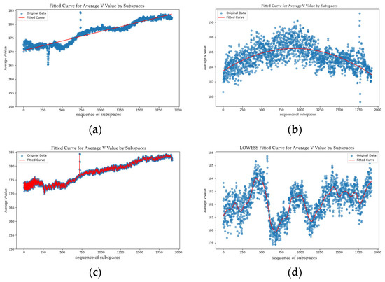
Figure 10.
(a) Linear Regression; (b) Polynomial Regression; (c) Spline Interpolation Fitting; (d) Locally Weighted Regression.
We ultimately selected LOWESS as the primary fitting strategy. LOWESS assigns weights to observations near each prediction point and performs localized regression analysis based on these weighted data, enabling precise modeling of local data characteristics. This method is particularly well-suited for datasets containing noise and outliers, effectively mitigating the influence of such disturbances. Moreover, LOWESS can adaptively adjust fitting parameters in response to local data variations, ensuring accurate fitting results even when the brightness curve exhibits significant fluctuations or abrupt changes.
4.4. Study on the Influence of Dynamic Subspace Range
This study designs DSFE to extract brightness features from fabric images, the range of the subspace inevitably affects the extraction results. A larger subspace tends to capture macroscopic brightness distributions, while a smaller one emphasizes finer, microscopic details. As discussed in Section 2, fabric defects are often caused by the misweaving of a single yarn. This implies that the dynamic subspace should not be excessively large. Moreover, during fabric image acquisition, phenomena such as moiré patterns, fabric unevenness, wrinkles, and stains often occur. If the subspace is too small, it may include excessive noise, thereby disturbing defect analysis. Therefore, the receptive field of the dynamic subspace should ideally encompass the defect itself along with two to three adjacent pixel columns. To investigate the effect of the subspace size on detection performance, we conducted a series of experiments. Figure 11 visualizes these results, and the detailed metrics are summarized in Table 2. Our experimental results demonstrate that a subspace size of 1.39 × 10⁻¹ dmm2 offers the optimal performance.
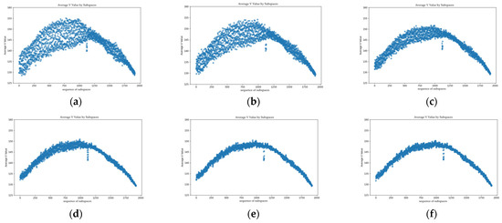
Figure 11.
Effect of subspace size on detection performance for values of: (a) 2.78 × 10⁻²; (b) 5.56 × 10⁻²; (c) 8.33 × 10⁻²; (d) 1.11 × 10⁻¹; (e) 1.39 × 10⁻¹; (f) 1.67 × 10⁻¹.
Table 2.
The table shows the effect of varying subspace range on detection performance.
4.5. Improvement of the Multidimensional Anomaly Analysis Formula
In terms of saliency representation, Equation (33) presents the classic SoftMax function, which is widely used to convert a set of values into a probability distribution. However, the traditional SoftMax formula is ill-suited for our application. It fails to account for the intrinsic disparities among different groups of values. When significant outliers are present, they disproportionately influence the calculation. This leads to a misrepresentation of the true differences between values.
To address this issue, we propose an improved formula based on the original SoftMax, Equation (34). Our formula incorporates an outlier scaling factor and a mean adjustment factor . This modification amplifies the influence of values significantly deviating from the data distribution while mitigating imbalance caused by extremes, resulting in a more reasonable and discriminative probability distribution (Figure 12).
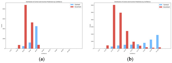
Figure 12.
(a) Traditional SoftMax formula; (b) improved SoftMax formula.
The improved formula enhances sensitivity to outliers. This ensures their saliency is distinctly reflected in the final output. Visualization results demonstrate that the optimized formula is better suited for complex scenarios requiring fine-grained differentiation among data points, it provides a more precise and reliable foundation for subsequent analysis.
In terms of dispersion characterization, we evaluated various statistical measures to quantify data dispersion, including Variance, Interquartile Range (IQR), Extremum, Coefficient of Variation (CV), and Peaks. The IQR and Extremum focus on extremes and fail to capture overall dispersion trends. The CV, though accounting for the mean, is sensitive to outliers and may produce misleading comparisons across datasets with varying scales. Peak value detection highlights salient local maxima but overlooks broader distribution characteristics.
In contrast, Variance effectively quantifies dispersion by averaging the squared deviations from the mean. As shown in Table 3, the data dispersion levels for the examples in the first column decrease sequentially. During this process, only variance shows a linear relationship with the degree of data dispersion. The other parameters exhibit no such linear regularity. Specifically, the variance value decreases as the degree of dispersion rises. It can accurately reflect the state of data dispersion. Moreover, variance maintains consistent expressiveness across different distribution patterns. Consequently, we selected variance as the preferred metric for measuring brightness dispersion in fabric images. This choice enables a precise characterization of the data distribution and an effective representation of changes in feature dispersion.
Table 3.
This table is based on Variance, IQR, Extremum, CV, Peaks calculation results of the method.
4.6. Comparison with Other Models
We constructed a small sample dataset by selecting 1104 images from the ZD001 dataset. Stratified random sampling was used to ensure the defect category distribution in the subset mirrored that of the original dataset. This process simulates the data-scarce scenarios common in industrial settings. This allows us to evaluate the model’s learning ability and generalization performance under such constraints. The small sample dataset was then split into training, validation, and test sets using an 8:1:1 ratio. For model performance evaluation, this study employs mean Average Precision (mAP) and Frames Per Second (FPS) as the core metrics. The mAP measures the overall performance of the model in multi-class detection tasks, while FPS assesses the model’s operational efficiency in practical industrial deployments. Together, these metrics provide a comprehensive evaluation framework for both detection accuracy and engineering applicability. By processing data with the CPU, our FPS is significantly higher than other models. Table 4 shows the parameter default values and ranges. The detection results of the various models are shown in Table 5.
Table 4.
This table shows the parameter default values and ranges.
Table 5.
This table shows the detection results of different models on the same dataset with small samples.
To validate our model’s stability, we reconstructed datasets of different sizes from the original 8795 images. We maintained the original class distribution throughout this process. Each dataset was then split into training, validation, and test sets at a ratio of 8:1:1. The experimental results are summarized in Table 6.
Table 6.
This table presents the training results following the adjustment of the dat-aset split.
Figure 13 presents the annotation results for different fabrics and defect types. In the figure, red boxes denote the manually annotated ground truths, green boxes represent algorithm-detected warp-direction defects, and blue boxes indicate weft-direction defects, with the detection confidence displayed alongside each bounding box. As can be observed, our method precisely localizes the defects and demonstrates strong robustness, as its performance is not compromised by common industrial artifacts such as oil stains and wrinkles.
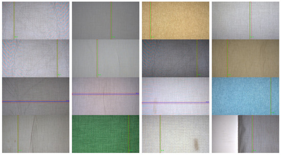
Figure 13.
Detection results for different defects.
4.7. Discussion
The experimental results compellingly demonstrate the effectiveness of our proposed multi-stage framework. Our method reliably identifies defects while remaining robust to interferences like wrinkles and stains. This addresses a significant challenge in automated textile inspection. This success can be attributed to the synergistic design of our components. First, the LFOA module reconstructs a uniform light field distribution. Simultaneously, the DSFE module extracts information-rich local features. Next, the anomaly characterization stage leverages LOWESS and our Outlier Index. This stage can sensitively detect even subtle deviations from the established norm. Finally, the adaptive optimization model provides an additional layer of robustness. It allows the system to fine-tune its sensitivity without manual intervention.
The significance of this work lies in its departure from data-intensive deep learning models. It offers a practical alternative for industrial settings where data is often scarce. Many conventional methods struggle with the trade-off between feature sensitivity and environmental robustness. In contrast, our approach provides a balanced solution.
Despite these promising results, this study has several limitations that open avenues for future research. Firstly, the current light field correction relies on a fixed template and does not yet adapt to the unique brightness characteristics of each individual image. Secondly, the feature extraction process is primarily optimized for warp and weft directional defects, with relatively limited effectiveness on highly localized, nonlinear defect shapes.
5. Conclusions
In this paper, we addressed the challenge of creating a data-efficient and robust defect detection method for the textile industry. We proposed a novel method based on dynamic subspace feature extraction, light field correction, and a texture-adaptive defect detection system that generates a probabilistic Outlier Index. Experimental results confirm that our method accurately localizes various fabric defects. It also exhibits strong resilience to common interferences like stains and wrinkles. Notably, it achieves high detection accuracy even with limited training samples, addressing key industrial challenges such as the rapid introduction of new textile varieties, the difficulty of sample acquisition, and poor model generalization. Furthermore, our model operates at a high detection speed. This makes it suitable for real-time inspection in industrial scenarios. Future work will focus on enhancing the adaptability of the light field correction and improving feature extraction for localized, non-directional defects.
Author Contributions
Conceptualization, W.W.; methodology, W.W.; software, Z.Z. and W.W.; validation, W.W.; formal analysis, Z.X. and M.Q.; investigation, W.W. and Z.Z.; resources, W.W.; data curation Z.X. and W.W.; writing—original draft W.W., Z.Z., Z.X. and M.Q.; writing—review and editing, W.W. and M.Q.; visualization W.W. and Z.Z.; supervision, Z.Z.; project administration Z.X.; funding acquisition, Z.X. All authors have read and agreed to the published version of the manuscript.
Funding
This work was supported by the National Key R&D Program of China (Grant No. 2023YFB3210901), the Pioneer and Leading Goose R&D Program of Zhejiang (Grant No. 2024C03118), the National Natural Science Foundation of China (Grant No. 52575602), the National Key R&D Program of China (Grant No. 2024YFB4614200), and Pioneer and Leading Goose R&D Program of Zhejiang (Grant No. 2025C01088).
Data Availability Statement
The data supporting the findings of this study are openly available in the Mendeley Data https://data.mendeley.com/datasets/7bw2hngcvz/1 (accessed on 9 April 2025).
Conflicts of Interest
The authors declare no conflicts of interest.
References
- Haralick, R.M.; Shanmugam, K.; Dinstein, I.H. Textural features for image classification. IEEE Trans. Syst. Man Cybern. 2007, SMC-3, 610–621. [Google Scholar] [CrossRef]
- Yu, G.; Zhang, F. Image recognition method for fabrics defects based on improved Res-UNet network. Wool Text. J. 2024, 52, 100–106. [Google Scholar]
- Dau Sy, H.; Thi, P.D.; Gia, H.V. Automated fabric defect classification in textile manufacturing using advanced optical and deep learning techniques. Int. J. Adv. Manuf. Technol. 2025, 137, 2963–2977. [Google Scholar] [CrossRef]
- Hu, G.; Wang, Q.; Zhang, G. Unsupervised defect detection in textiles based on Fourier analysis and wavelet shrinkage. Appl. Opt. 2015, 54, 2963–2980. [Google Scholar] [CrossRef]
- Li, Y.; Luo, H.; Yu, M. Fabric defect detection algorithm using RDPSO-based optimal Gabor filter. J. Text. Inst. 2018, 110, 487–495. [Google Scholar] [CrossRef]
- Rue, H.; Tjelmeland, H. Fitting Gaussian Markov random fields to Gaussian fields. Scand. J. Stat. 2002, 29, 31–49. [Google Scholar] [CrossRef]
- Cohen, F.S.; Fan, Z.; Attali, S. Automated Inspection of Textile Fabrics Using Textural Models. IEEE Trans. Pattern Anal. Mach. Intell. 1991, 13, 803–808. [Google Scholar] [CrossRef]
- Brzakovic, D.; Bakic, P.R.; Vujovic, N. A generalized development environment for inspection of web materials. In Proceedings of the International Conference on Robotics and Automation, Albuquerque, NM, USA, 25 April 1997; pp. 1–8. [Google Scholar]
- Zhao, X.; Wang, L.; Zhang, Y. A review of convolutional neural networks in computer vision. Artif. Intell. Rev. 2024, 57, 99. [Google Scholar] [CrossRef]
- Mienye, I.D.; Swart, T.G.; Obaido, G. Recurrent neural networks: A comprehensive review of architectures, variants, and applications. Information 2024, 15, 517. [Google Scholar] [CrossRef]
- Pu, Q.; Xi, Z.; Yin, S. Advantages of transformer and its application for medical image segmentation: A survey. Biomed. Eng. Online 2024, 23, 14. [Google Scholar] [CrossRef] [PubMed]
- Ameri, R.; Hsu, C.-C.; Band, S.S. A systematic review of deep learning approaches for surface defect detection in industrial applications. Eng. Appl. Artif. Intell. 2024, 130, 107717. [Google Scholar] [CrossRef]
- Jia, Z.; Wang, M.; Zhao, S. A review of deep learning-based approaches for defect detection in smart manufacturing. J. Opt. 2024, 53, 1345–1351. [Google Scholar] [CrossRef]
- Wu, S.; Xiong, Y.; Cui, Y. Retrieval-augmented generation for natural language processing: A survey. arXiv 2024, arXiv:2407.13193. [Google Scholar] [CrossRef]
- Yang, S.; Wang, Z.; Wu, W. Research Progress on Automatic Image Annotation Technology. J. Detect. Control. 2025, 47, 24–32+40. [Google Scholar]
- Khan, U.A.; Javed, A. A hybrid CBIR system using novel local tetra angle patterns and color moment features. J. King Saud Univ.-Comput. Inf. Sci. 2022, 34, 7856–7873. [Google Scholar] [CrossRef]
- Yang, J.; Xing, C.; Chen, Y. Improving the ScSPM model with Log-Euclidean Covariance matrix for scene classification. In Proceedings of the 2016 International Conference on Computer, Information and Telecommunication Systems (CITS), Kunming, China, 6–8 July 2016; pp. 1–5. [Google Scholar]
- Zhu, T.; Li, S.; He, X. WCE Polyp Detection Based On Locality-Constrained Linear Coding with A Shared Codebook. In Proceedings of the 2020 IEEE 9th Data Driven Control and Learning Systems Conference (DDCLS), Liuzhou, China, 20–22 November 2020; pp. 404–408. [Google Scholar]
- Yu, J.; Huang, D.; Li, J. Parallel Acceleration of Real-time Feature Extraction Based on SURF Algorithm. In Proceedings of the 2023 15th International Conference on Computer Research and Development (ICCRD), Hangzhou, China, 10–12 January 2023; pp. 57–63. [Google Scholar]
- Maharjan, P.; Vanfossan, L.; Li, Z. Fast LoG SIFT Keypoint Detector. In Proceedings of the 2023 IEEE 25th International Workshop on Multimedia Signal Processing (MMSP), Poitiers, France, 27–29 September 2023; pp. 1–5. [Google Scholar]
- Gavkare, S.; Umbare, R.; Shinde, K. Identification and Categorization of Brain Tumors Using HOG Feature Descriptor. In Proceedings of the 2023 IEEE International Conference on Blockchain and Distributed Systems Security (ICBDS), New Raipur, India, 6–8 October 2023; pp. 1–6. [Google Scholar]
- Liu, W.; Anguelov, D.; Erhan, D. Ssd: Single shot multibox detector. In Proceedings of the Computer Vision—ECCV 2016: 14th European Conference, Amsterdam, The Netherlands, 11–14 October 2016; Proceedings, Part I 14. pp. 21–37. [Google Scholar]
- Tan, M.; Pang, R.; Le, Q.V. EfficientDet: Scalable and Efficient Object Detection. In Proceedings of the 2020 IEEE/CVF Conference on Computer Vision and Pattern Recognition (CVPR), Seattle, WA, USA, 13–19 June 2020; pp. 10778–10787. [Google Scholar]
- Redmon, J.; Divvala, S.; Girshick, R. You Only Look Once: Unified, Real-Time Object Detection. In Proceedings of the 2016 IEEE Conference on Computer Vision and Pattern Recognition (CVPR), Las Vegas, NV, USA, 27–30 June 2016; pp. 779–788. [Google Scholar]
- Liu, C.; Gao, G.; Liu, Z. Fabric Defect Detection Algorithm Based on Multi-channel Feature Extraction and Joint Low-Rank Decomposition. In Image and Graphics; Lecture Notes in Computer Science; Springer International Publishing: Berlin/Heidelberg, Germany, 2017; pp. 443–453. [Google Scholar]
- Zhang, B.; Tang, C. A Method for Defect Detection of Yarn-Dyed Fabric Based on Frequency Domain Filtering and Similarity Measurement. Autex Res. J. 2019, 19, 257–262. [Google Scholar] [CrossRef]
- Xu, S.; Cheng, S.; Jin, S. Industrial Fabric Defect-Generative Adversarial Network (IFD-GAN): High-fidelity fabric cross-scale defect samples synthesis method for enhancing automated recognition performance. Eng. Appl. Artif. Intell. 2025, 161, 112296. [Google Scholar] [CrossRef]
- Wang, Y.; Xiang, Z.; Wu, W. MCF-Net: A multi-scale context fusion network for real-time fabric defect detection. Digit. Signal Process. 2025, 167, 105425. [Google Scholar] [CrossRef]
- Xiang, Z.; Jia, J.; Zhou, K. Block-wise feature fusion for high-precision industrial surface defect detection. Vis. Comput. 2025, 41, 9277–9295. [Google Scholar] [CrossRef]
- Zhou, K.; Jia, J.; Wu, W. Space-depth mutual compensation for fine-grained fabric defect detection model. Appl. Soft Comput. 2025, 172, 112869. [Google Scholar] [CrossRef]
- Xiang, Z.; Shen, Y.; Ma, M. HookNet: Efficient Multiscale Context Aggregation for High-accuracy Detection of Fabric Defects. IEEE Trans. Instrum. Meas. 2023, 72, 5016311. [Google Scholar] [CrossRef]
- Xu, S.; Cheng, S.; Jin, S.Y.; Hu, X.D.; Wu, W.T.; Xiang, Z. “ZD001”. Mendeley Data, Version 1; Zhejiang Sci-Tech University: Hangzhou, China, 2025. [Google Scholar] [CrossRef]


Disclaimer/Publisher’s Note: The statements, opinions and data contained in all publications are solely those of the individual author(s) and contributor(s) and not of MDPI and/or the editor(s). MDPI and/or the editor(s) disclaim responsibility for any injury to people or property resulting from any ideas, methods, instructions or products referred to in the content. |
© 2025 by the authors. Licensee MDPI, Basel, Switzerland. This article is an open access article distributed under the terms and conditions of the Creative Commons Attribution (CC BY) license (https://creativecommons.org/licenses/by/4.0/).