Abstract
Student dropout remains a persistent challenge in higher education, with substantial personal, institutional, and societal costs. We developed a modular dropout prediction pipeline that couples data preprocessing with multi-model benchmarking and a governance-ready explainability layer. Using 17,883 undergraduate records from a Moroccan higher education institution, we evaluated nine algorithms (logistic regression (LR), decision tree (DT), random forest (RF), k-nearest neighbors (k-NN), support vector machine (SVM), gradient boosting, Extreme Gradient Boosting (XGBoost), Naïve Bayes (NB), and multilayer perceptron (MLP)). On our test set, XGBoost attained an area under the receiver operating characteristic curve (AUC–ROC) of 0.993, F1-score of 0.911, and recall of 0.944. Subgroup reporting supported governance and fairness: across credit–load bins, recall remained high and stable (e.g., <9 credits: precision 0.85, recall 0.932; 9–12: 0.886/0.969; >12: 0.915/0.936), with full TP/FP/FN/TN provided. A Shapley additive explanations (SHAP)-based layer identified risk and protective factors (e.g., administrative deadlines, cumulative GPA, and passed-course counts), surfaced ambiguous and anomalous cases for human review, and offered case-level diagnostics. To assess generalization, we replicated our findings on a public dataset (UCI–Portugal; tables only): XGBoost remained the top-ranked (F1-score 0.792, AUC–ROC 0.922). Overall, boosted ensembles combined with SHAP delivered high accuracy, transparent attribution, and governance-ready outputs, enabling responsible early-warning implementation for student retention.
1. Introduction
It has long been considered that student dropout is one of the most problematic and protracted issues affecting educational organizations around the world. Besides resulting in personal losses to students such as less career potential, unsound finances, and reduced social mobility, the phenomenon also takes its toll on the society and the institution in terms of resource wastage, worse performance, and lower contributions to social and economic development. As online and hybrid education is gaining momentum very rapidly, especially in the current situation of digital transformation and dependence on learning management systems, the need to manage early student withdrawal challenges is becoming even more acute. Higher education institutions (HEIs) must handle large volumes of student data because of digitalization, which demands data-driven methods to detect at-risk students and deliver immediate interventions.
Machine learning (ML) has become a game-changing force in a range of fields that combines predictive power with practical decision support. In agriculture, ML is being integrated into smart farm platforms to fine-tune crop management, monitor soils, and forecast yields to drive sustainable climate-resilient practices [1]. In healthcare, ML models improve disease diagnosis, personalize treatments, and guide population health management showing an ability to sift through medical data with greater accuracy and efficiency [2]. Beyond these areas, ML finds use in everything, from cybersecurity and smart city infrastructures to business intelligence and educational settings, strengthening its cross-sector relevance in the Fourth Industrial Revolution [3]. When viewed as a whole, these deployments illustrate the wide-reaching power of ML to confront problems highlighting the need for interpretable and governance-ready frameworks, especially for high-stakes tasks, like forecasting dropout rates in higher education.
Attention mechanisms have swiftly become a cornerstone of deep learning models letting them latch onto the salient cues while drowning out the irrelevant noise. Recent surveys put a spotlight on the reach of attention mechanisms. In their 2021 review, Correia and Colombini [4] unpack the building blocks and design choices, behind attention underscoring its relevance for natural-language processing, vision and multimodal applications. Brauwers and Frasincar [5] follow up with a taxonomy that not categorises the various attention styles but also offers evaluation frameworks and draws parallels across disciplines. Meanwhile Hassanin et al. [6] dive into visual-attention techniques outlining the architectural families (channel, spatial and self-attention) that dominate contemporary computer-vision models. Collectively the body of work showcases the flexibility and interpretability of attention mechanisms hinting at ground for future applications, in educational data analytics especially where intricate temporal and relational dependencies must be captured.
In the last ten years, data mining and artificial intelligence (AI) research in the field of education and learning has made significant progress, and machine learning models are being developed to predict student dropout more accurately and earlier. Systematic reviews indicate that hundreds of factors have been reported to have an impact on student dropout, varying between academic performance and social economic status to institutional and individual factors [7].
Nevertheless, despite this heterogeneity, research is highly biased toward academic and demographic variables, which are simple to compute, while psychological, motivational, and behavioral predictors are often neglected. Not only this, but interpretability has failed to keep up with the increase in predictive accuracy, and only a small proportion of studies have relied on explainable artificial intelligence processes, i.e., Shapley additive explanations (SHAP) and Local Interpretable Model-agnostic Explanations (LIME). This has led to the development of models that are difficult to implement as practical policies for teachers and administrators, thereby raising questions about the real-world usefulness of models that are merely accurate.
Recent advancements in the discipline, however, have demonstrated that more effective solutions can be achieved. For example, Alghamdi, Soh, and Li [8] designed ISELDP, which includes a stacking ensemble architecture in which Adaptive Boosting (AdaBoost), random forest, gradient boosting, and Extreme Gradient Boosting (XGBoost) along with a multilayer perceptron as a meta-learner are incorporated, and they reported a significant improvement in predictions of in-session dropout. Their experiment demonstrated that the proposed ensemble-based architecture has the potential to address the phenomenon of class imbalance and support real-time predictive analytics of at-risk learners, but the magnitude of computation, generalization, and explanation issues remain within this organization as a means of delivery of learning data applications within a learning environment. Similarly, Bañeres et al. [9] implemented an extensive early-warning system (EWS) at the Universitat Oberta de Catalunya, where the gradual at-risk (GAR) system has the potential to deliver continuous predictions and instantaneous responses to the early stages of student activity in a course. This model shows how the combination of a predictive model and interventional mechanisms, i.e., nudges and an instructor dashboard, can assist in a see-saw increase in retention. However, there are several drawbacks to the approach because of its dependence on the grades of continuous assessments, as well as the fact that it lacks generalizability to other administrative cases of examination.
Besides system-level deployments, there is an increasing amount of work on the importance of explainability in dropout prediction. Padmasiri and Kasthuriarachchi [10] investigated interpretable dropout prediction models through the integration of machine learning predictors with SHAP and LIME to identify which variables including tuition history, age, and academic grades most impact dropout status. Their user evaluation found that educators valued the interpretability of these models, but the study still has shortcomings, as it only used one dataset and a small sample of professionals. Similarly, Islam et al. [11] combined several explainable artificial intelligence (XAI) methods within an educational data-mining model to allow both global and local interpretability and to detect the key factors, such as their Kernel Tuning Toolkit (KTT) usage, scholarship, and unemployment rates. The literature demonstrates a growing trend toward decision–support systems that provide actionable insights instead of opaque predictive models, yet scalability, dataset diversity, and longitudinal validation remain major challenges.
There have also been applications of comparative analysis to the role that methodological choice plays in dropout prediction. The authors of [12] demonstrated that support vector regression, gradient boosting, and XGBoost outperform basic models after performing extensive hyperparameter optimization. The research by Villar and de Andrade [13] demonstrated that the Categorical Boosting (CatBoost) and Light Gradient Boosting Machine (LightGBM) algorithms, together with SHAP analysis, achieved superior F1-scores and better dropout driver identification than standard methods. The results show a general trend in research because ensemble and deep learning models always produce better predictive results. However, such methods require more computational power, which increases the risk of overfitting, particularly when working with small or unbalanced datasets.
The predictive horizons are expanding in new directions. Models now aim to identify dropout risk not just in higher education but also much earlier in the student lifecycle. Psyridou et al. [14] demonstrated that dropout can be predicted as early as the end of primary school using balanced random forests trained on a 13-year longitudinal dataset. Their research showed that reading fluency, comprehension, and early arithmetic skills are among the strongest predictors of future dropout risk. This demonstrates the significance of early interventions. Similarly, Martinez, Sood, and Mahto [15] stressed the importance of engagement and behavioral characteristics in the detection of dropout in real time in higher education. They showed that the Naïve Bayes and random forest models can achieve a precision greater than in small pilot deployments. The research demonstrates how dropout develops over time through academic and cognitive factors, as well as behavioral and contextual elements. The success of an intervention depends on both the early identification of problems and the continuous assessment of the situation.
Research has made significant progress, but there are still important research gaps. The continuous data imbalance problem reduces the reliability of predictive models. Minority dropout cases are often ignored by classifiers in favor of the majority non-dropout cases. The risk of overfitting remains high in ensemble and deep learning frameworks because they require complex hyperparameter tuning. Research findings have not been validated across different institutions, cultural settings, or academic fields. The field of explainable AI has received significant attention, but most existing research focuses on post hoc feature attribution methods rather than designing models that incorporate understanding from the start. The literature does not contain systematic methods to differentiate between risk and protection factors, which is necessary for developing complete proactive intervention strategies.
It is against this background that the present study was conducted. Based on prior solutions to ensemble learning, explainable AI, and EWSs, we developed a modular dropout prediction pipeline. The system evaluates classical, ensemble, and deep learning models with explainability integrated into the core of the pipeline. SHAP-based analysis helps achieve two goals: it enables global feature importance analysis and detects anomalies, understands ambiguity, and identifies high-confidence misclassifications. Our method delivers practical insights that surpass black-box prediction through the risk versus protection factor distinction. We strive to provide educators and policymakers tools that are both comprehensible and practical. This research demonstrates how methodological complexity leads to real-world application through scientific rigor, thus producing practical solutions to fight student dropout. We use “dropout” to denote eventual non-completion within the observation window, “at-risk” to indicate positive predictions, and “withdrawal” for institution-specific administrative codes.
This work contributes a modular, reproducible pipeline that benchmarks nine classifiers on 17,883 Moroccan undergraduate records and couples them with a governance-ready SHAP layer; statistically grounded comparisons showing XGBoost as the top model on our test set (area under the receiver operating characteristic curve (AUC–ROC) , F1-score , and recall ), with significance testing against strong peers; subgroup reporting (credit–load, division, and major) with full true positives, true negatives, false positives, and false negatives for governance and fairness auditing; case-level explanations that surface anomalous/ambiguous predictions for human-in-the-loop review; and an external replication on the “Predict Students’ Dropout and Academic Success” public dataset [16], indicating preserved ranking and generalization of the approach.
2. Related Work
Educational data mining (EDM) and learning analytics (LA) have placed dropout prediction at their center because it represents both a societal and an institutional crisis. Research into predictive methods for educational purposes started with basic classifiers and continued with advanced deep learning and XAI frameworks over the last 15 years. The field has advanced with two primary objectives: to enhance predictive accuracy, as well as to transform predictions into practical interventions. The literature demonstrates ongoing challenges, which include accuracy issues, along with interpretability problems and scalability limitations. This review examines previous studies in three main categories: machine learning, deep learning, and explainable AI. The following section reveals the current knowledge gaps.
The development of dropout prediction started with research using case studies to demonstrate machine learning applications in educational settings. Yükseltürk et al. [17] implemented k-nearest neighbors (k-NN), decision trees, Naïve Bayes, and neural networks for dropout prediction in Turkish online certificate students. The models showed sensitivity results of 87% for k-NN and 79.7% for decision trees, establishing that predictive analytics work for identifying at-risk students. The study employed self-reported questionnaires about readiness, locus of control, and self-efficacy, but these instruments may have generated biased results. The dataset contained only 189 participants while being cross-sectional and specific to online education, thus making the findings less applicable to other contexts. Dekker et al. [18] performed one of the first extensive case studies in the Netherlands through decision tree classifiers to forecast first-year dropout in electrical engineering students. The predictive models achieved accuracy rates between 75% and 80% because academic performance data from linear algebra and calculus demonstrated the most predictive value. They introduced cost-sensitive learning methods, which decreased false-positive rates to prevent the unnecessary exclusion of potential success candidates. Their focus on academic grades as predictors resulted in overlooking motivational and socioeconomic factors, while data quality problems and external validation issues affected the study. Earlier work established the practical application of EDM but demonstrated difficulties in working with limited datasets and limited feature diversity alongside poor interpretability.
2.1. Machine Learning for Dropout Prediction
Most studies on dropout prediction in low-resource environments depend on classical machine learning approaches because deep learning models are impractical in these contexts. Hassan et al. [19] applied random forests and other supervised learning methods to Somaliland national survey information. The models achieved accuracy levels of 95% through the identification of age, grade level, and school type, along with housing conditions, as key predictive variables. The research gained attention because it used a large dataset that supported educational policy decisions. The study used static cross-sectional data, yet this method raised doubts about data stability across time and it prioritized demographic factors over psychological and behavioral indicators.
The study by El Mahmoudi et al. [20] investigated Moroccan public university dropout rates using logistic regression along with support vector machine (SVM), k-NN, and decision trees. The research results showed that academic performance does not stand alone as a dropout factor since students’ relationships with professors and their motivation levels and socioeconomic conditions play a significant role. The study analyzed data from 120 students, but its statistical analysis power remained weak, while the lack of explainable AI made it difficult for administrators to apply the model’s predictions.
Research studies have investigated particular algorithms in greater depth. Panizales et al. [21] applied Naïve Bayes classifiers to online learning platforms to prove that basic probabilistic models can efficiently identify risks at large scale. The effectiveness of Naïve Bayes in particular situations is limited because it requires independent features but fails when multiple variables show strong correlation. The research by Kuntintara et al. [22] examined various ML models using Bangkok University data, showing that XGBoost achieved the highest predictive accuracy by surpassing 84% precision and recall thresholds. The study demonstrated the increasing effectiveness of ensemble tree-based methods. The investigation confined its analysis to a single educational institution, yet failed to employ interpretability methods, which resulted in stakeholders receiving unclear answers. The research by Chen et al. [23] focused on feature selection through decision trees and random forest, alongside SVM and neural networks, using first-year student data. The study confirmed academic and enrollment factors as critical predictive elements, but it neglected psychological aspects, failed to validate findings in real time, and lacked external dataset integration. This research demonstrates that although classical ML functions adequately with small, organized datasets, it continues to face two critical barriers through its dependence on academic and demographic factors, alongside its interpretability issues.
2.2. Deep Learning Approaches
The growth of big data alongside digital learning environments has made deep learning necessary for dropout prediction. Kalita et al. [24] developed a bidirectional long short-term memory Bi-LSTM system that combines sequence modeling capabilities with SHAP-based interpretability methods. The approach showed excellent results in outcome prediction, and attendance, grades, and student engagement were found to be important factors. The research showed that deep learning methods can benefit from interpretability techniques. The analysis of small datasets created overfitting issues, and SHAP interpretation methods required significant computational resources. Alnasyan et al. [25] developed Kanformer, which uses attention-based mechanisms combined with Kolmogorov–Arnold networks (KANs) and multi-head attention mechanisms. The evaluation of Open University Learning Analytics Dataset (OULAD) datasets revealed that Kanformer performed better than Transformer models, while providing easy-to-understand feature importance scores. The high computational requirements for training and inference operations, along with complex model architecture, make it unsuitable for institutions with limited infrastructure capabilities.
The application of deep learning techniques has been evaluated in massive open online courses (MOOCs) because these platforms generate substantial clickstream data. Yang et al. [26] showed that convolutional neural networks (CNNs) and long short-term memory network (LSTM) architectures outperform traditional classifiers because they can detect sequential behavior patterns. The research demonstrated that engagement and interaction features are important but also revealed certain constraints. The lack of explainable AI integration in black-box models makes instructors question their trustworthiness, and platform-specific log reliance creates barriers for model transferability between different contexts. Kakarla et al. presented a comparison between artificial neural networks and traditional ML algorithms. The study by [27] showed that artificial neural networks (ANNs) perform better than traditional ML algorithms in detecting nonlinear patterns. The analysis of their small dataset increased the possibility of overfitting, and their models lacked both institutional transferability and interpretability capabilities. Deep learning research demonstrates better accuracy and pattern recognition capabilities yet faces obstacles related to computational expenses, transparency, and general applicability.
2.3. Gap Synthesis
Research has made progress, but multiple gaps continue to exist in the existing literature. The models of Hassan’s Somaliland survey [19] and El Mahmoudi’s Moroccan study [20] demonstrate high accuracy in their specific settings, yet they fail to transfer effectively between institutions, cultures, and different educational levels. The Bi-LSTM [24] and Kanformer [25] deep learning models demonstrate high accuracy, but their high computational requirements and tendency to overfit make them impractical for educational settings. Additionally, interpretability is still lacking. SHAP and LIME have gained popularity, but researchers typically implement them as additional components after model development instead of incorporating them into the initial model framework, and their effectiveness for non-technical users remains uncertain [28,29]. The development of reliable EWSs requires anomaly detection, ambiguity analysis, and longitudinal validation methods, yet these methods remain underutilized. The distinction between risk factors (dropout-related variables) and protective factors (dropout-reducing variables) remains unclear in most studies, although this distinction is vital for developing student-centered interventions. Recent studies [30,31] have reaffirmed the strength of tree ensembles on structured higher education institution (HEI) data but have stopped short of integrating governance diagnostics, subgroup fairness tables, and external replication within a single modular framework.
The current study builds upon previous machine learning research [17,18] and essential XAI frameworks [32,33,34] to address the identified gaps. Our research enhances both methodological quality and practical use through the evaluation of classical, ensemble, and deep learning models in a modular system and the implementation of SHAP-based analyses for feature attribution and anomaly detection and ambiguity analysis. The research identifies both risk and protective factors. The research provides useful insights that exceed black-box predictions and delivers reliable, easy-to-understand tools that match the needs of educators and policymakers in their specific contexts.
3. Materials and Methods
3.1. Data Collection and Preprocessing
We assembled a longitudinal institutional dataset of undergraduate records spanning multiple cohorts at a Moroccan HEI. Each row corresponds to a unique student and integrates demographic and program descriptors, academic progression, engagement/attendance, financial/administrative signals, and a rich family of administrative holds coded as pattern-matched columns:
where each HAS_XX flags whether hold XX ever applied, and the paired timestamps delimit its active window. All such HAS_* variables are holds. Notably, HAS_AP indicates a pre-registration hold; its window AP_START_DTE/AP_END_DTE can block enrollment until resolved Throughout, and we normalize all timestamps to elapsed days. Durations such as AP_END_DTE − AP_START_DTE are included as continuous features.
HAS_XX , XX _START_DTE, XX _END_DTE,
The raw files display typical EDM issues: inconsistent delimiters, date/time fields, high missingness in a subset of administrative columns, and categorical identifiers with leakage risk. Following established practice [17,18,35], we applied (i) automatic delimiter detection; (ii) column removal at >90% missingness [36]; (iii) median imputation for numeric fields; (iv) label encoding for categoricals with an explicit <MISSING> token; (v) date normalization to days-since-reference; and (vi) leakage prevention by dropping direct identifiers (ID_NUM) and anonymizing advisor codes.
The target STUDENT_STATUS was binarized as a supervised classification label, in line with prior work [17,18]:
Students on academic leave remain labeled 0 (persist/graduate) unless administratively withdrawn by the registrar. Some administrative hold codes (HAS_*) are institution specific, while academic performance features (e.g., GPA, credits, and failures) are broadly transferable across HEIs. Ground-truth outcomes were taken from the institution’s registrar outcome field STUDENT_STATUS at the end of the observation window defined for this study. Labels were assigned post hoc with no access to model features at inference time: indicates students recorded by the registrar as having eventually discontinued studies (dropout), while denotes students who persisted or graduated within the window. The outcome field was used solely to define y and was not included among predictor features. After cleaning and curation, the modeling matrix comprised students and features. The positive class contained 2856 students (16.0%). We used a stratified 80/20 split, yielding 14,306 training and 3577 test students (positives ≈ 2285 train/571 test). Class imbalance informed the evaluation choices (ROC thresholded metrics) and motivated post hoc explainability to support case review and governance. A compact summary follows in Table 1.

Table 1.
Dataset statistics after cleaning and feature preparation.
3.2. Proposed Pipeline
To ensure reproducibility and modularity, we designed a structured pipeline that combines all stages of the dropout prediction task, from raw data ingestion to interpretability analysis. This pipeline follows the principles of transparent and reproducible machine learning research in education [35,37]. It was implemented entirely in Python 3.12.0 using open-source libraries like scikit-learn 1.7.1, xgboost 3.0.3, and shap 0.48.0.
Figure 1 shows the modular architecture. The workflow starts with data ingestion and preprocessing as described in Section 3.1. Cleaned features go into a model benchmarking module where a diverse set of algorithms are trained and evaluated, which range from classical statistical learners to modern ensemble and neural models. Next, an explainability layer based on SHAP values is applied to extract actionable insights. These include risk and protective factors, unusual cases, and uncertain predictions. Finally, metrics, visualizations, and logs are exported to structured output directories for clear auditing.

Figure 1.
Modular pipeline for dropout prediction and interpretability. The pipeline consists of six stages: (1) data ingestion and preprocessing, (2) feature engineering, (3) model training and evaluation, (4) explainability analysis using SHAP, (5) anomaly and ambiguity detection, and (6) visualization and reproducibility.
The pipeline includes reproducibility as one of its main characteristics. The single entry script manages all experiments by storing random seeds together with cross-validation folds, missingness thresholds, and SHAP sampling caps in a configuration file. The setup enables the complete duplication of results between different operating environments. The approach fulfills current demands for educational data science transparency according to [38]. The system records all experimental settings together with dataset statistics, including missing data rates and class distribution and model parameters. The system stores artifacts, including confusion matrices, receiver operating characteristic (ROC) curves, SHAP plots, and performance summaries, in versioned directories for traceability purposes.
The pipeline structure with separate modules for preprocessing, modeling, and interpretability enables both flexibility through new model additions and LIME implementation and comparability for algorithm evaluation within a unified framework.
Notation conventions: Bold symbols denote vectors (e.g., ), plain italics denote scalars, and probabilities are written as .
3.3. Models
The predictive modeling stage of this study examined multiple algorithms, which included classical statistical models together with ensemble methods and neural networks. We selected this broad range to achieve equilibrium between model understanding and predictive accuracy in our research. This is a common focus in dropout prediction research [39,40,41]. The two basic models that are easy to understand and interpret are logistic regression and Naïve Bayes. Gradient boosting and multilayer perceptrons demonstrate superior prediction performance, yet their interpretability remains challenging. A direct comparison of these methods enables us to assess their effectiveness in addressing the dropout issue.
Logistic regression (LR) is the most commonly used baseline for classification problems in educational data mining [42]. It estimates the probability of a student dropping out as
where is the sigmoid function, refers to the coefficients learned from data, and b is the intercept. The coefficients provide direct insights into how each variable affects dropout risk.
Decision trees (DTs) [40] partition the feature space into smaller, homogeneous regions by recursively splitting attributes that maximize an impurity reduction criterion, such as Gini impurity:
where is the proportion of class k in node t. Trees are highly interpretable, allowing educators to visualize decision rules, but they often suffer from overfitting when used alone.
Random forests (RFs) [39] mitigate this weakness by averaging predictions over multiple bootstrapped decision trees, thereby reducing variance. RFs have shown consistent robustness in dropout studies due to their ability to handle noisy and high-dimensional data.
Naïve Bayes (NB) classifiers [43] apply Bayes’s theorem under a conditional independence assumption:
which, despite its simplicity, makes NB efficient for categorical predictors frequently present in educational datasets (e.g., major codes and honors status).
The k-nearest neighbors (k-NN) classifier [44] predicts student outcomes by majority voting among the k closest training instances. While k-NN adapts naturally to complex decision boundaries, its performance depends heavily on the choice of distance metric and k, and it can be computationally expensive on large datasets.
Support vector machines (SVMs) [45] construct a hyperplane that maximizes the margin between dropout and non-dropout classes. For input , the classifier computes
where is the feature vector, is the weight vector (normal to the hyperplane), is the bias term, and returns if and otherwise (here, denotes dropout and non-dropout). The decision boundary is given by . SVMs are particularly effective in high-dimensional spaces but can be less interpretable than tree-based methods.
Ensemble models combine multiple learners to achieve stronger predictive power. Gradient boosting (GB) [46] builds models in an additive way, fitting new learners to the leftover errors of earlier models. Its strength lies in managing nonlinear relationships and unbalanced datasets, which are common in dropout situations where the number of students who stay is much higher than those who drop out.
XGBoost [41] improves GB with second-order optimization, shrinkage, and clear regularization. Its objective function is
where indexes training instances , indexes the boosted trees, is the true label (1 = dropout, 0 = non-dropout), is the ensemble’s raw score (logit under logistic loss), is a pointwise loss (e.g., logistic/cross-entropy), is the k-th regression tree, T is its number of leaves, are its leaf weights, penalizes additional leaves, and controls regularization on the leaf weights. XGBoost has been widely reported to outperform traditional models in educational data mining [7].
Multilayer perceptrons (MLPs) [47] represent the neural baseline in our benchmark. An MLP consists of multiple fully connected layers, where each hidden unit computes
where is the input feature vector, is the weight matrix for a hidden layer of m units, is the bias vector, is the resulting hidden activations, and is the nonlinear activation function (e.g., rectified linear unit (ReLU) or sigmoid). The final output layer applies a sigmoid to estimate dropout probabilities. Although less transparent than logistic regression or decision trees, MLPs capture higher-order interactions among features such as GPA trends, probation history, and withdrawal counts. This flexibility makes them suitable for capturing nonlinear dropout patterns.
The models used in this study aim to balance performance and interpretability. Logistic regression and Naïve Bayes offer clear baselines that help with straightforward policy interpretation. Decision trees and random forests provide decent interpretability while effectively managing various feature types. Gradient boosting and XGBoost serve as top benchmarks for tabular classification tasks, showcasing strong predictive power, though they are more complex. Lastly, including MLPs ensures we cover neural approaches, allowing us to compare different learning methods. Overall, this variety in methods helps us find the most accurate predictors and evaluate which models offer useful insights for educators and policymakers. For completeness, the symbols used across metrics appear in Table 2.
Table 2.
Notations used for classification metrics and predictions.
3.4. Evaluation Metrics
The evaluation of predictive models for student dropout detection needs the careful selection of performance metrics. This requirement arises from the imbalanced datasets, where non-dropout cases greatly outnumber dropout cases. Relying only on overall accuracy can be misleading. A model biased toward predicting the majority class might have high accuracy while still failing to identify students at risk. For this reason, this study used a set of complementary evaluation measures. These measures focus on both overall classification performance and the ability to detect minority outcomes.
Let be the ground-truth label for student i (1 = dropout; 0 = persist/graduate), and let be the model’s predicted probability of dropout. A hard label is obtained via a decision threshold as ; we selected on the validation folds to maximize F1 and then fixed it for test reporting and subgroup tables. Based on the pairs , we computed the confusion matrix cells (true positives (TP), true negatives (TN), false positives (FP), and false negatives (FN)) which underpin all reported metrics.
Because dropout was the minority class in our data (≈16%), overall accuracy could be misleading; we therefore emphasized class-sensitive metrics. The definitions we used are
To summarize threshold-independent separability, we report AUC-ROC, where the ROC traces TPR versus FPR across all and
Under class imbalance, precision–recall (PR) analysis is often more informative; we therefore cite the area under the precision–recall curve (PR-AUC) where appropriate but, to align with the implemented pipeline, we report thresholded metrics (precision, recall, and F1) together with AUC-ROC.
To ensure stability and generalizability, model performance was validated using stratified k-fold cross-validation. In each fold, the dataset was partitioned into training and testing subsets, and the F1-score was computed. The mean and standard deviation across folds,
are reported to quantify not only central tendency but also variability in performance [36]. Cross-validation thus guards against overfitting to a single data split and provides a robust estimate of real-world predictive performance.
Overall, the evaluation framework emphasizes metrics that address both class imbalance and the asymmetric costs of misclassification. Accuracy alone is insufficient, and greater weight is placed on precision, recall, F1, and cross-validated F1. These measures ensure not only that the models classify correctly in aggregate but also, more importantly, that they capture the complex dynamics of dropout risk in a way that is actionable for educational institutions [7].
3.5. Model Validation and Statistical Testing
Model selection and variability were assessed on the training partition using stratified folds with a fixed global seed (42) so that all models saw identical folds. Within each fold, we trained on 4/5 of the training set and validated on the remaining 1/5, preserving the empirical class ratio. For thresholded metrics, we selected a single operating threshold per model by maximizing F1 on the validation predictions aggregated across folds; this was then fixed and applied to the remaining test set and to all subgroup summaries. As descriptive stability measures, we report the mean and standard deviation of cross-validated F1 (CV-F1 mean ± std) computed on the fold-level validation splits. For linear and margin-based learners (LR/DT/RF/SVM), we used built-in class weighting balanced on the training folds; tree-boosting used scale_pos_weight matched to the training positive/negative ratio, as listed in Table 3. We audited probability calibration with reliability plots on validation predictions and found no systematic over/under-confidence that would justify post hoc recalibration; to keep models comparable, we therefore did not apply Platt/Isotonic scaling and relied on the single threshold selected as above.
Table 3.
Training setup and hyperparameters (final settings used for the test set models).
After cross-validation, each model was retrained on the full training set (same hyperparameters) and evaluated once on the untouched test set. We report the accuracy, precision, recall, F1, AUC-ROC, and CV-F1 mean±std (Table 4). Confusion matrices at the operating threshold appear in Figure 2 and Figure 3. To assess whether top-model differences are meaningful on the same test instances, we used McNemar’s test on paired predictions. Let b be the number of test samples misclassified by model A but correctly classified by model B, and c vice versa; concordant cells are ignored. The McNemar statistic (without continuity correction) is
with b and c declared in Table 2. We report exact two-sided p-values with the tuple and (Table 5). Because we performed two pairwise comparisons among the top models within a dataset (XGBoost vs. random forest; XGBoost vs. gradient boosting), we additionally note that the qualitative conclusions were unchanged under a Holm–Bonferroni correction at : on our institutional test split, XGBoost vs. gradient boosting remained significant (), while XGBoost vs. random forest did not (). For completeness, we also report a simple paired discordant error rate as an effect-size proxy,
interpreted as the net proportion of disagreements favoring model B (negative values favor A). We emphasize that these tests assessed paired classification differences on this particular sample; they do not replace external validation.
Table 4.
Performance of all models on the dropout prediction task. Test set metrics are reported alongside five-fold, cross-validated F1-scores (mean ± standard deviation) computed on the training set.
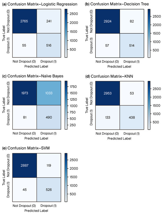
Figure 2.
Confusion matrices (classical models) at the operating threshold used in Table 4. Cells show counts of TP, FP, FN, and TN; darker shading indicates higher counts. False negatives (FNs) are critical in early-warning use (missed at-risk students).
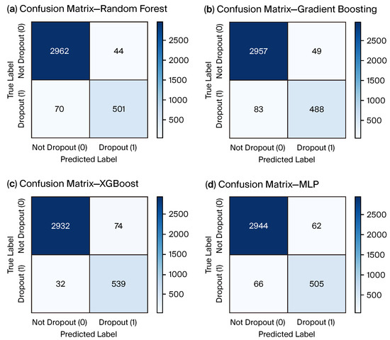
Figure 3.
Confusion matrices (ensembles and neural) at the same operating threshold as Figure 2.
Table 5.
Paired significance (McNemar) for top models on held-out test sets. b: A wrong, B correct; c: A correct, B wrong; . Two-sided exact p-values reported.
3.6. Fairness and Subgroup Reporting Protocol
Operational deployment requires visibility into group-wise error trade-offs. We therefore computed, on the held-out test set and at the fixed operating threshold selected on cross-validation, the following per-subgroup quantities: precision, recall (TPR), false negative rate (FNR), and the full confusion matrix cells (TP, FP, FN, and TN). Subgroups were limited to routinely collected academic variables to avoid attribute inference: (i) credit–load bins, (ii) academic division codes, and (iii) program/major. Division codes were anonymized institutional identifiers (e.g., “1” and “3”); the program variable (MAJOR_1) was label encoded and reported as integer codes to preserve anonymity (textual names were withheld). Summaries for this study appear in Table 6, Table 7 and Table 8.
Table 6.
This study’s (XGBoost) performance by credit–load bin (A2).
Table 7.
This study’s (XGBoost) performance by division (encoded).
Table 8.
This study’s (XGBoost) performance by major (encoded). Metrics use the single global threshold fixed on cross-validation. Small-n categories yield unstable estimates.
Consistent with our governance posture, we intentionally restricted subgroup auditing to academic operational variables (credit load, division, and major) and did not include gender or socioeconomic status, which were neither available nor approved for analysis in this study; we also did not infer such protected attributes.
To ensure comparability, we applied a single global threshold per model to all subgroups. This isolates genuine performance differences from subgroup-specific thresholding effects. Where governance requires subgroup-specific actions, we recommend documenting any deviation from the global , with pre-/post-metrics archived.
In addition to raw metrics, we tracked simple disparity indicators declared in Table 2 such as
and flag any subgroup with FNR materially exceeding the overall FNR.
3.7. External Replication Dataset
To evaluate transferability beyond a single HEI, we replicated the entire pipeline on a public higher-education dataset [16] (“Predict Students’ Dropout and Academic Success”). After standard cleaning and label mapping (“Dropout” ; “Enrolled”/“Graduate” ), the prepared matrix contained N = 4424 students and 36 tabular features with a class distribution of 3003 non-dropout vs. 1421 dropout (32.1%). Preprocessing matched the institutional study: Columns with >90% missingness were dropped; numeric missing values were median imputed; categoricals were label encoded with an explicit <MISSING> token; and dates were normalized where available. We used the same 80/20 stratified split (3539 train, 885 test), the same model menu and hyperparameters (Table 3), identical cross-validation and threshold-selection protocols, and the same evaluation metrics.
3.8. Explainability Layer
Beyond predictive accuracy, how well models can be understood is important in education. The outcomes of classification directly influence student support and retention policies. A model that is very accurate but hard to understand may not gain the trust of educators or policymakers. This lack of trust can hinder its use [32,34]. To address this issue, the current study added an explanation layer based on SHAP [33]. This layer offers both overall interpretability and specific explanations for individual cases.
SHAP is grounded in cooperative game theory, where the prediction of a machine learning model for a single instance is distributed among its input features. For a model f and input vector , the SHAP value for feature j represents the average marginal contribution of that feature across all possible feature coalitions . Formally, the contribution is defined as
where denotes the model restricted to features in S, and the weighting term corresponds to the Shapley value formulation, ensuring fairness among features [33]. SHAP additive decomposition achieves local accuracy and missingness and consistency properties, which establishes it as one of the most theoretically sound explainability techniques available.
This study used SHAP values to analyze top-performing models, producing both global importance rankings that show the most influential predictors across the population and local explanations that explain individual dropout predictions. The global explanations showed which features are always risk and protection factors for dropout predictions. The analysis showed different patterns in the local area because some students received high-confidence misclassifications, which the explainability layer detected as abnormal profiles. Following recommendations by the recent explainable AI literature [33,34], we further characterized ambiguous cases, defined as instances with predicted dropout probabilities close to the decision boundary (), and high-confidence wrong predictions, where was large despite . These phenomena illustrate how interpretability can serve as a diagnostic tool for model reliability.
The integration of SHAP enables domain experts to view prediction logic, which enhances both the reproducibility and trustworthiness of educational machine learning applications. SHAP provides a distinct framework that maintains global consistency and local faithfulness, whereas traditional feature importance methods such as permutation importance and gain-based tree model measures only deliver global summaries [33]. The practical implementation of this method helps teachers distinguish between individual student problems and institutional vulnerabilities to identify specific factors like total credit hours, attendance records, and probation status that affect dropout predictions. The explainability layer enables responsible student success initiative predictive analytics implementation through model output connections to educational insights that drive action [32,34].
4. Results
4.1. Model Performance
Table 4 provides a summary of all classifiers’ experimental results. In order to ensure robustness against overfitting, the models were further assessed using five-fold cross-validation after being trained on historical student data that was 80/20 stratified into training and test sets. Accuracy, precision, recall, F1-score, the AUC-ROC, and the mean and standard deviation of the cross-validated F1-score were used to gauge performance. With dropout cases making up only approximately 16% of the population, this combination of metrics offers a comprehensive evaluation of predictive ability in the presence of class imbalance.
The ensemble-based classifiers performed better than traditional machine learning models according to the results presented in Table 4. Strong sensitivity to dropout cases is indicated by the recall of 0.904 obtained by logistic regression; however, more false positives were generated by its comparatively low precision of 0.682. The results match previous studies demonstrating that linear models tend to overpredict minority classes in educational datasets that are unbalanced [48]. The F1-score of decision tree models reached 0.881 compared to ensembles, while offering better interpretability but reduced generalization potential. The random forest classifier reached an F1-score of 0.898 and an AUC-ROC of 0.989 when multiple trees were used for bagging to achieve a suitable balance between recall and precision. This is in line with previous research that highlights the resilience of tree ensembles in student dropout detection [49,50].
The support vector machine (SVM) achieved an F1-score of 0.865 and maintained one of the highest recalls (0.921) to detect minority dropout cases in high-dimensional feature spaces. The training process and computational expenses for tree-based ensembles exceeded those of other methods. Gradient boosting achieved F1 = 0.881 and AUC-ROC = 0.988, slightly below random forest (F1 = 0.898, AUC-ROC = 0.989), because sequential boosting refines the decision boundary [46]. The multilayer perceptron (MLP) achieved an F1-score of 0.888 and an AUC-ROC of 0.979, showing that neural architectures can detect complex nonlinearities in student progress data but at the expense of reduced interpretability [51].
The XGBoost model achieved the highest F1-score (0.911), recall (0.944), and AUC-ROC (0.993) among all models. The model achieved better results because of its enhanced regularization capabilities and its ability to detect high-order feature interactions, as well as its optimized handling of imbalanced data through weighted loss functions. Recent real-world implementations corroborate these findings. For instance, Carballo-Mendívil et al. developed an XGBoost-based EWSs using pre-enrollment data from almost 40,000 students, which proved its ability to detect at-risk students early with high sensitivity and useful insights [52]. General reviews in educational data mining show that ensemble techniques such as bagging, boosting, and stacking outperform individual classifiers in terms of predictive accuracy and robustness, especially when it comes to performance or student dropout prediction [53]. However, when applied to highly correlated academic features, the Naïve Bayes classifier performed poorly (F1-score = 0.468), indicating the limitations of its strong independence assumptions [43]. As summarized in Table 9, XGBoost remains the top-ranked (F1-score , AUC-ROC ), with logistic regression and gradient boosting close behind, corroborating preserved model ordering under a different data source.
Table 9.
Public dataset replication model performance on the test set.
Building on the aggregate metrics in Table 4 and Table 5 compares paired test errors for the top models. In this study, XGBoost showed fewer unique errors than gradient boosting (McNemar ), while the difference compared to random forest was not statistically significant (). On the public dataset [16], XGBoost remained the top-ranked with no significant gap versus random forest or gradient boosting, consistent with Table 9. Notably, the public dataset lacked institution-specific administrative hold features; nevertheless, the ensemble models retained their advantage on purely academic/demographic signals, supporting generalization of the modeling stack and thresholding procedure under feature shift. Together, these findings indicate that our pipeline transfers across sources while maintaining coherent model ordering and governance-ready outputs.
Subgroup results by credit load (Table 6) showed consistently high recall across bins (0.932–0.969) with low FNR (3.1–6.8%), indicating that the screening sensitivity of XGBoost was stable across enrollment intensities. The division-level results (Table 7) retained high recall in the largest unit (code 3: 0.956) and acceptable recall in the smaller unit (code 1: 0.855), suggesting no pronounced sensitivity drop with scale. Very small categories can yield unstable metrics due to few positive cases and should be interpreted with caution or aggregated for governance reporting. At the major level (Table 8), using the label-encoded MAJOR_1 variable, the three largest groups (codes 49, 2, 12; ) sustained high recall at solid precision (code 49: precision , recall , FNR ; code 2: ; code 12: ; detailed TP/FP/FN/TN in the table). Several small-n majors (e.g., codes 20, 27, 23, 11, 28, and 24) showed perfect or near-perfect scores but had few positives, so estimates are unstable.
Our analysis showed that interpretable baseline models, including decision trees and logistic regression, provide useful information yet ensemble methods deliver superior performance than these models. XGBoost exhibited the most promising predictive ability. The ensemble methods provide the most reliable combination of overall predictive reliability and sensitivity to dropout cases for operational early-warning systems in higher education. The high recall of XGBoost makes it suitable for early intervention frameworks because it is more important to minimize false-negative missed dropout cases than to attain perfect precision.
4.2. Visualizations
We offer a collection of visualizations that showcase model performance in terms of classification reliability and ranking ability in order to supplement the numerical results that are displayed. In the context of dropout prediction, these graphical representations help us better understand the trade-offs between sensitivity and specificity, as well as assessing the error distribution across models.
A clear picture of how each classifier allocates predictions among the true and predicted classes is provided by confusion matrices. They show where each model tends to make mistakes by exposing the balance between true positives, false positives, true negatives, and false negatives. This representation is particularly helpful for determining the prevalence of false negatives, which are the most serious mistakes in early-warning systems because they correspond to at-risk students who are not identified, in highly unbalanced settings like dropout detection. All benchmarked models’ confusion matrices are shown in Figure 2 and Figure 3, which makes it easy to see the relative advantages and disadvantages of each strategy.
The confusion matrix summarizes performance at a specific decision threshold, whereas ROC curves provide threshold-independent insight into separability. AUC-ROC offers a single, threshold-independent summary, while each ROC curve traces the trade-off between true-positive and false-positive rates across thresholds. Because ROC can look optimistic under strong class imbalance, we paired ROC curves with thresholded metrics (precision, recall, and F1) and confusion matrices. In this study, we report ROC-only ranking plots, as our implemented outputs generated ROC figures exclusively.
The ROC curves for each classifier are shown in Figure 4. Naïve Bayes exhibited the weakest separability, while the ensemble methods (gradient boosting, random forest, and especially XGBoost) produced curves closest to the upper-left corner with the highest AUC-ROC values.
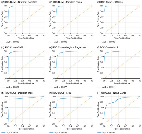
Figure 4.
ROC curves. Legends report AUC-ROC. Curves nearer the upper-left corner indicate stronger separability between dropout and non-dropout classes.
Together, ROC curves and confusion matrices provide complementary views: ROC summarizes ranking quality across thresholds, while the confusion matrix reveals the error balance (TP, FP, TN, and FN) at the operating threshold used to report test set metrics.
4.3. Explainability Outcomes
To understand the internal logic of the top-performing models and ensure that predictive performance rests on educationally meaningful signals, we conducted a SHAP-based analysis. Across models, AP_END_DTE emerged as the dominant predictor, with mean absolute SHAP values of ≈1.902 for XGBoost, ≈0.1007 for random forest, and ≈0.112 for MLP (values reported on the held-out test set). This variable acts as a structural timing signal for dropout risk, especially when extreme values co-occur with moderate/declining performance and administrative enrollment deadlines. CAREER_GPA and PASSED_CRS_COUNT consistently ranked in the top features, aligning with prior evidence that academic momentum drives both attrition and persistence [37,38].
The top ten risk and protective features across models are shown in Figure 5. Major risk factors included course failures, cumulative GPA deficits, and late administrative deadlines; protective factors included timely advisor engagement proxies and stable term credit loads. Magnitudes on the risk side exceeded those on the protective side, suggesting that sharp negative shocks tend to precipitate dropout more than gradual supports prevent it.
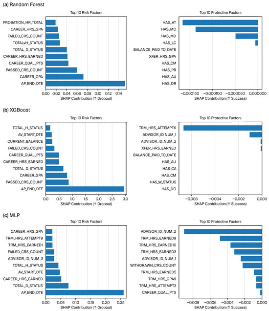
Figure 5.
Top ten SHAP-derived risk and protective features across XGBoost, random forest, and MLP. Positive values increase dropout probability; negative values are protective.
Global SHAP summary plots (Figure 6) show that XGBoost concentrates most predictive weight in a compact set dominated by AP_END_DTE, PASSED_CRS_COUNT, TOTAL_D_STATUS, CAREER_GPA, and CAREER_HRS_EARNED. Random forest exhibits a similar but slightly more diffuse pattern, while the MLP shows a broader spread of attributions, reflecting its nonlinear representation. Such concentration reduces the dimensionality needed to explain risk attribution, yielding predictions that are easier for institutional stakeholders to interpret.
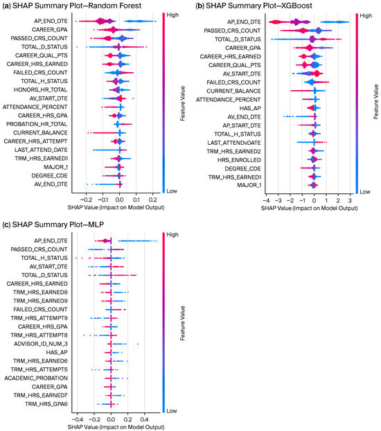
Figure 6.
Top SHAP-derived risk features: (a) Random Forest, (b) XGBoost, and (c) MLP on the test set. The x-axis is the SHAP value (log-odds): values > 0 increase predicted dropout risk, values < 0 are protective; dot color encodes the feature value (low → high, blue → pink).
At the case level, ∼5% of students presented as anomalous (high SHAP complexity relative to their predicted probability): 179/3576 for XGBoost and 179/3576 for random forest; for MLP, which was analyzed on a standardized 300-sample subset, anomalies were 15/300 (5%). Ambiguous mid-probability cases were numbered 40 (XGBoost), 74 (random forest), and 2 (MLP); high-confidence misclassifications were 66, 34, and 9, respectively. For example, student #15280 was flagged primarily due to a strongly negative AP_END_DTE contribution (≈−3.70), despite otherwise average metrics. As shown in Figure 7, these diagnostics indicate where human review is warranted before action.
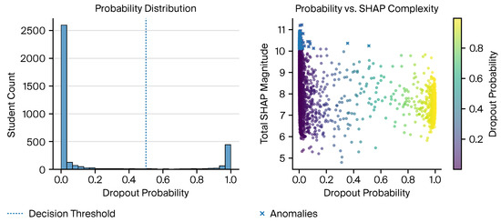
Figure 7.
XGBoost probability distribution (left) and (right) total SHAP magnitude vs. predicted dropout probability; points are colored by dropout probability (color bar: low → high). Points with unusually high SHAP complexity relative to predicted probability are flagged as anomalous; mid-probability cases () are marked as ambiguous for human review.
Overall, SHAP not only reveals which characteristics drive predictions but also surfaces boundary cases where predictions may be unreliable. This enables early-warning systems to avoid blind reliance on algorithmic outputs and to embed human-in-the-loop review for transparency and equity [33].
4.4. Case-Level Validation
Table 10 summarizes a representative case, labeled A3 (number 15280), and shows the aligned prediction and ground truth. For student A3, the XGBoost model yielded a dropout probability of and a predicted label of 0, matching the true label (0∣0). The top local SHAP drivers were AP_END_DTE (), CAREER_HRS_EARNED (), and TOTAL_D_STATUS (). As noted in the table, the drivers indicated protective administrative timing and accumulated credits; human review was retained for edge cases.
Table 10.
A3 case summary (this study).
5. Discussion
This study’s empirical findings support a trend repeatedly reported in the dropout-prediction literature: ensemble tree methods outperform linear, probabilistic, and shallow baselines on heterogeneous institutional data. On our held-out test set (3577 students; dropout rate 16%), XGBoost achieved AUC-ROC , F1-score , and recall , surpassing gradient boosting and random forest. An SVM also performed competitively (AUC ) but trailed behind the tree ensembles in recall at comparable false-positive rates. Logistic regression displayed a steeper recall–precision trade-off, and Naïve Bayes suffered from very low precision despite moderate recall, consistent with prior findings on class-imbalanced tabular data [23,39,41,46].
5.1. Explaining the Performance Differences
The inductive biases of the models explain why they performed differently. The linear decision boundaries of logistic regression, together with other models, depend on the assumption of monotonic additive log-odds of dropout [42]. The assumptions made by such models become invalid when risk depends on complex relationships between cumulative GPA, administrative deadlines, and course completion counts. The problem is magnified by the Naïve Bayes’s assumption of conditional independence between features [43], which is often not true in educational records where achievement, attendance, and engagement are correlated. In contrast, nonlinear decision surfaces are constructed by tree-based models. Gradient boosting machines [46] and XGBoost [41] incrementally fit residuals to approximate high-order effects and sparse feature combinations, while random forests [39] use bagging to reduce variance. Their superior recall and balanced precision—recall performance in imbalanced domains like dropout detection, where the minority positive class is of primary institutional concern—are directly explained by this inductive flexibility.
5.2. Comparisons with Contemporary Work
Our findings are positioned in relation to four very recent 2025 contributions in Table 11. A convergent picture shows that tree ensembles and finely tuned classical machine learning techniques continue to be the state of the art for dropout prediction on structured higher education data, despite differences in dataset sizes, feature availability, and methodological decisions. Panizales et al. [21] tested Naïve Bayes on 1000 online learning records and pointed out that the assumptions of independence and class imbalance sensitivity are major problems. They found that the model had strong accuracy (93%) but very weak recall for dropouts (53%). Pérez et al. [30] used a dataset of 8737 students from Ecuador to verify random forest and XGBoost as the top models (accuracy ≈ 96.6%, F1-score ≈ 0.94). The surprising result was that preprocessing interventions like PCA or SMOTE worsened performance, showing the importance of maintaining the tabular feature structure. Mojumder Anik et al. [54] used survey data () and focused on Bangladesh, where they obtained good results for SVM and LightGBM, but the small sample size limits generalizability and introduces self-report bias. Last but not least, Abdullah et al. [31] used multiple sources of data (, 35 features) to propose a random forest and gradient boosting ensemble, which reached 93.5% accuracy and AUC = 0.97 but at the cost of higher computational complexity and reduced interpretability. Unlike recent tree-ensemble baselines [30,31], our pipeline integrates governance diagnostics (covering anomaly/ambiguity/high-confidence wrong predictions), subgroup fairness tables at a global , and external replication all within one reproducible stack.
Table 11.
Recent studies on student dropout prediction: datasets, best models, metrics, interpretability, and limitations.
A direct comparison of headline metrics can be found in Table 12. In addition to outperforming published results in accuracy and F1, our XGBoost classifier has the highest recall among its peers. Because false negatives (missed at-risk students) have disproportionate institutional costs, it is particularly important for early-warning contexts to be able to maintain high recall at non-trivial precision levels in the precision–recall space [55,56].
Table 12.
Headline metrics on our held-out test set (3577 students) versus representative literature.
5.3. Interpretability Insights
The ensemble methods present complexity, but SHAP analysis revealed that predictions rely on a small number of stable features, including AP_END_DTE, CAREER_GPA, PASSED_CRS_COUNT, and TOTAL_D_STATUS. The XGBoost model assigned AP_END_DTE the highest mean absolute SHAP value of ≈1.902, followed by PASSED_CRS_COUNT (≈0.721), TOTAL_D_STATUS (≈0.555), CAREER_GPA (≈0.521), and CAREER_HRS_EARNED (≈0.409). The results match previous research that identified GPA and semester completion as the primary risk factors [30,37,38]. The pipeline delivered three major interpretability breakthroughs: (i) risk vs. protective factor decomposition identified elements that lead to failure and elements that promote persistence; (ii) anomaly and ambiguity detection revealed that ≈5% of students exhibited unusually high SHAP magnitude in relation to probability, and ≈1% students formed ambiguous mid-probability clusters. The new developments address major limitations in current research because most studies rely on raw feature importance (e.g., [30,31]) instead of post hoc XAI techniques ([33,34,57]).
5.4. Ethical and Governance Considerations
Risks to equity, openness, and student autonomy must be balanced against the advantages of highly effective predictive models. First, process artifacts may be encoded by administrative codes or hold timestamps; ablation and counterfactual probes [58] are necessary to ensure that predictions are not dependent on factors beyond the student’s control. Second, to make sure that false-negative or false-positive rates are not disproportionately distributed across demographic or program subgroups, group fairness should be explicitly assessed using equalized odds-style assessments [59]. Third, we contend that explicit cost models that weigh the effects of missed interventions against over-intervention should be used to determine prediction thresholds. Lastly, we emphasize that post hoc explanations (like SHAP) are not a replacement for intrinsically interpretable models where decisions are legally binding, echoing Rudin [60] and Lipton [61]. Therefore, our framework supports a hybrid approach: boosted ensembles for accurate screening but always integrated into human-in-the-loop decision pipelines, with documented review pathways and informed student consent. These precautions guarantee that predictive analytics strengthen institutional legitimacy and trust rather than erode it.
5.5. Summary of Contributions
In conclusion, our discussion places the empirical benefits of boosted tree methods in the context of both the normative demands of higher education governance and the technical environment of dropout prediction. Our contributions to the recent literature are threefold: (1) a tabular-first, high-performing modeling stack that generalizes across HEI data; (2) an interpretability layer that includes protective vs. risk factors, global SHAP, and anomaly detection; and (3) explicit governance and fairness recommendations that position predictive models as tools for decision support rather than decision replacement. When combined, these components provide a reliable and practical guide for responsible early-warning systems in higher education.
6. Conclusions and Future Work
This research used ensemble trees alongside neural networks and traditional linear classifiers to create and evaluate a modular system for student dropout prediction. We contribute three things: The evaluation of nine classifiers on historical student data revealed that XGBoost and gradient boosting tree-based ensemble models delivered the best results for all accuracy, recall, F1-score, and AUC performance metrics. The second part of our approach used Shapley additive explanations (SHAP) as a unifying interpretability layer to demonstrate that the most predictive models select their choices based on educationally significant factors, including administrative deadlines and cumulative GPA and progression indicators. The third improvement included diagnostic lenses for explainability analysis to identify abnormal profiles, uncertain probability ranges, and confident misclassifications.
The results showed that researchers need to achieve an equilibrium point that combines model interpretability with predictive accuracy. Although the gradient boosting family produces better ranking quality, its use in educational settings is only warranted when combined with clear explanations that enable stakeholders to confirm the consistency of risk factors and take appropriate action in response to them. The results were not statistical errors because we used confusion matrices, ROC analyses, and SHAP attributions to demonstrate that they produced consistent and understandable patterns in student data. The available information allowed for the creation of warning systems during the initial stages.
However, it is important to recognize a number of limitations. Some predictors (e.g., administrative hold timestamps such as AP_START_DTE and AP_END_DTE) are institution specific and may not exist or have the same semantics elsewhere. Division and program variables are reported in encoded form; several majors/divisions have small sample sizes, so subgroup estimates can be unstable and should be interpreted with caution or aggregated for governance reporting. Our fairness audit was intentionally restricted to routinely collected academic variables (credit load, division, and major); we did not infer or analyze protected attributes (e.g., gender or socioeconomic status). Although replication on a public dataset preserved model ordering, broader multi-institution validation remains necessary. The SHAP framework provided strong results but operated as an approximation that could have introduced biases from the models used for analysis. The research focused on tabular features, so it did not include the temporal dynamics and relational structures that define student trajectories.
Accordingly, we position the pipeline as a screening aid within a documented, human-in-the-loop workflow. Institutions should apply a single global threshold per model, archive subgroup metrics for audit, and avoid automating high-stakes decisions from model scores alone. Three research paths that support each other should be explored in the future. The continuous-time models neural ordinary differential equations (neural ODEs) and neural neural controlled differential equations (neural CDEs) track student performance and engagement metrics through their ability to detect early warning signs by analyzing time-dependent patterns in student data. The second method employs relational data between students, classes, and teachers to identify structural factors that affect persistence through graph-based learning techniques. Third, in order to help advisors and policymakers take prompt and fair action, deployment research should focus on creating real-time institutional dashboards that combine interpretable visualizations with predictive scores. The implementation of these methods can help produce dependable early-warning systems that maintain transparency, ethical standards, and flexibility for adapting to changing higher education requirements.
Author Contributions
Conceptualization, A.B. and F.-Z.B.; methodology, A.B.; software, A.B.; validation, A.B., F.-Z.B. and H.H.; formal analysis, A.B.; investigation, A.B.; resources, H.H.; data curation, A.B.; writing—original draft preparation, A.B.; writing—review and editing, F.-Z.B. and H.H.; visualization, A.B.; supervision, H.H.; project administration, H.H.; funding acquisition, F.-Z.B. and H.H. All authors have read and agreed to the published version of the manuscript.
Funding
This research received no external funding.
Institutional Review Board Statement
Not applicable.
Informed Consent Statement
Not applicable.
Data Availability Statement
The data used in this study were obtained from internal student records of a Moroccan higher education institution and cannot be shared publicly due to privacy and ethical restrictions. Derived datasets and aggregated results are available from the corresponding author upon reasonable request.
Acknowledgments
The authors thank the institutional data team for secure data access.
Conflicts of Interest
The authors declare no conflicts of interest.
Abbreviations
The following abbreviations are used in this manuscript:
| AI | Artificial Intelligence |
| ANN | Artificial Neural Network |
| AP | (Administrative) Pre-registration Hold |
| AUC | Area Under the Curve |
| AUC-ROC | Area Under the Receiver Operating Characteristic Curve |
| Bi-LSTM | Bidirectional Long Short-Term Memory |
| CatBoost | Categorical Boosting |
| CDE | Controlled Differential Equation |
| CV | Cross-validation |
| DT | Decision Tree |
| EDM | Educational Data Mining |
| EWS | Early-Warning System |
| FPR | False-Positive Rate |
| GB | Gradient Boosting |
| GDPR | General Data Protection Regulation |
| GPA | Grade Point Average |
| HEI | Higher Education Institution |
| KAN | Kolmogorov–Arnold Network |
| k-NN | k-Nearest Neighbors |
| LA | Learning Analytics |
| LightGBM | Light Gradient Boosting Machine |
| LIME | Local Interpretable Model-agnostic Explanations |
| LR | Logistic Regression |
| ML | Machine Learning |
| MLP | Multilayer Perceptron |
| MOOC | Massive Open Online Course |
| NB | Naïve Bayes |
| ODE | Ordinary Differential Equation |
| PCA | Principal Component Analysis |
| PR | Precision–Recall |
| PR-AUC | Area Under the Precision–Recall Curve |
| RF | Random Forest |
| ReLU | Rectified Linear Unit |
| ROC | Receiver Operating Characteristic |
| SHAP | Shapley Additive Explanations |
| SMOTE | Synthetic Minority Oversampling Technique |
| SVM | Support Vector Machine |
| TabNet | Interpretable Deep Tabular Learning Network |
| TPR | True-Positive Rate |
| XAI | Explainable Artificial Intelligence |
| XGB | XGBoost (Extreme Gradient Boosting) |
References
- Araújo, S.O.; Peres, R.S.; Ramalho, J.C.; Lidon, F.; Barata, J. Machine Learning Applications in Agriculture: Current Trends, Challenges, and Future Perspectives. Agronomy 2023, 13, 2976. [Google Scholar] [CrossRef]
- An, Q.; Rahman, S.; Zhou, J.; Kang, J.J. A Comprehensive Review on Machine Learning in Healthcare Industry: Classification, Restrictions, Opportunities and Challenges. Sensors 2023, 23, 4178. [Google Scholar] [CrossRef]
- Sarker, I.H. Machine Learning: Algorithms, Real-World Applications and Research Directions. SN Comput. Sci. 2021, 2, 160. [Google Scholar] [CrossRef] [PubMed]
- Correia, M.; Colombini, E.L. Attention, please! A survey of Neural Attention Models in Deep Learning. arXiv 2021, arXiv:2103.16775. [Google Scholar] [CrossRef]
- Brauwers, G.; Frasincar, F. A General Survey on Attention Mechanisms in Deep Learning. ACM Comput. Surv. 2023, 55, 1–42. [Google Scholar] [CrossRef]
- Hassanin, M.; Anwar, S.; Radwan, I.; Khan, F.S.; Mian, A. Visual Attention Methods in Deep Learning: An In-Depth Survey. Expert Syst. Appl. 2024, 235, 121107. [Google Scholar] [CrossRef]
- Quimiz-Moreira, M.; Delgadillo, R.; Parraga-Alava, J.; Maculan, N.; Mauricio, D. Factors, prediction, explainability, and simulating university dropout through machine learning: A systematic review, 2012–2024. Computation 2025, 13, 198. [Google Scholar] [CrossRef]
- Alghamdi, S.; Soh, B.; Li, A. ISELDP: An enhanced dropout prediction model using a stacked ensemble approach for in-session learning platforms. Electronics 2025, 14, 2568. [Google Scholar] [CrossRef]
- Bañeres, D.; Rodríguez, M.E.; Guerrero-Roldán, A.E.; Karadeniz, A. An early warning system to detect at-risk students in online higher education. Appl. Sci. 2020, 10, 4427. [Google Scholar] [CrossRef]
- Padmasiri, P.; Kasthuriarachchi, S. Interpretable prediction of student dropout using explainable AI models. In Proceedings of the International Research Conference on Smart Computing and Systems Engineering (SCSE), Colombo, Sri Lanka, 3 April 2024; pp. 1–7. [Google Scholar] [CrossRef]
- Islam, M.M.; Sojib, F.H.; Mihad, M.F.H.; Hasan, M.; Rahman, M. The integration of explainable AI in educational data mining for student academic performance prediction and support system. Telemat. Inform. Rep. 2025, 18, 100203. [Google Scholar] [CrossRef]
- Demirtürk, B.; Harunoğlu, T. A comparative analysis of different machine learning algorithms developed with hyperparameter optimization in the prediction of student academic success. Appl. Sci. 2025, 15, 5879. [Google Scholar] [CrossRef]
- Villar, A.; de Andrade, C.R.V. Supervised machine learning algorithms for predicting student dropout and academic success: A comparative study. Discov. Artif. Intell. 2024, 4, 2. [Google Scholar] [CrossRef]
- Psyridou, M.; Prezja, F.; Torppa, M.; Lerkkanen, M.-K.; Poikkeus, A.-M.; Vasalampi, K. Machine learning predicts upper secondary education dropout as early as the end of primary school. arXiv 2024, arXiv:2403.14663. [Google Scholar] [CrossRef]
- Martinez, A.L.J.; Sood, K.; Mahto, R. Early detection of at-risk students using machine learning. In Foundations of Computer Science and Frontiers in Education: Computer Science and Computer Engineering; Springer Nature: Cham, Switzerland, 2025; pp. 396–406. [Google Scholar] [CrossRef]
- Realinho, V.; Vieira Martins, M.; Machado, J.; Baptista, L. Predict Students’ Dropout and Academic Success [Dataset]. UCI Mach. Learn. Repos. 2021, 10, C5MC89. [Google Scholar] [CrossRef]
- Yukselturk, E.; Ozekes, S.; Turel, Y.K. Predicting dropout student: An application of data mining methods in an online education program. Eur. J. Open Distance e-Learn. 2014, 17, 118–133. [Google Scholar] [CrossRef]
- Dekker, G.W.; Pechenizkiy, M.; Vleeshouwers, J.M. Predicting students drop out: A case study. In Proceedings of the 2nd International Conference on Educational Data Mining (EDM), Cordoba, Spain, 1–3 July 2009; pp. 41–50. [Google Scholar]
- Hassan, M.A.; Muse, A.H.; Nadarajah, S. Predicting student dropout rates using supervised machine learning: Insights from the 2022 national education accessibility survey in Somaliland. Appl. Sci. 2024, 14, 7593. [Google Scholar] [CrossRef]
- El Mahmoudi, A.; Chaoui, N.E.H.; Chaoui, H. Predictive analytics leveraging a machine learning approach to identify students’ reasons for dropping out of university. Appl. Sci. 2025, 15, 8496. [Google Scholar] [CrossRef]
- Panizales, W.; Lagunzad, H.; Ferrer, M.; Villanueva, C.; Kalaw, D.; Garcia, K. Predicting student dropout rates in online education platforms utilizing Naive Bayes algorithm. In Proceedings of the 16th International Conference on E-Education, E-Business, E-Management and E-Learning (IC4e), Tokyo, Japan, 26–29 April 2025; pp. 425–429. [Google Scholar] [CrossRef]
- Kuntintara, W.; Warabuntaweesuk, P.; Rattapasakorn, S. Student dropout prediction using machine learning. In Proceedings of the 9th International Conference on Business and Industrial Research (ICBIR), Bangkok, Thailand, 23–24 May 2024; pp. 229–233. [Google Scholar] [CrossRef]
- Chen, L.-S.; Huynh-Cam, T.-T.; Nalluri, V.; Lu, T.-C.; Agrawal, S. Determining important features for first-year student dropouts using artificial intelligence algorithms. In Proceedings of the 6th International Workshop on Artificial Intelligence and Education (WAIE), Tokyo, Japan, 28–30 September 2024; pp. 128–133. [Google Scholar] [CrossRef]
- Kalita, E.; Alfarwan, A.M.; El Aouifi, H.; Kukkar, A.; Hussain, S.; Ali, T.; Gaftandzhieva, S. Predicting student academic performance using Bi-LSTM: A deep learning framework with SHAP-based interpretability and statistical validation. Front. Educ. 2025, 10, 1581247. [Google Scholar] [CrossRef]
- Alnasyan, B.; Basheri, M.; Alassafi, M.; Alnasyan, K. Kanformer: An attention-enhanced deep learning model for predicting student performance in virtual learning environments. Soc. Netw. Anal. Min. 2025, 15, 25. [Google Scholar] [CrossRef]
- Yang, S.; Xiao, Y.; Meng, F. Deep learning-based method for predicting student dropouts in MOOCs. In Proceedings of the 7th International Conference on Machine Learning and Natural Language Processing (MLNLP), Chengdu, China, 18–20 October 2024; pp. 1–6. [Google Scholar] [CrossRef]
- Kakarla, S.; Mahany, D. Implementation of artificial neural networks and machine learning algorithms to evaluate and predict educational student dropout metrics. In Proceedings of the 6th International Workshop on Artificial Intelligence and Education (WAIE), Tokyo, Japan, 28–30 September 2024; pp. 102–106. [Google Scholar] [CrossRef]
- Castro, R.Q.; Garcia, K.C.; Jarrin, E.P. Predictive modeling and explainability for academic dropout risk detection using machine learning. In Proceedings of the Eleventh International Conference on eDemocracy & eGovernment (ICEDEG), Bern, Switzerland, 18–20 June 2025; pp. 114–122. [Google Scholar] [CrossRef]
- Silva, F.d.C.; Santana, A.M.; Feitosa, R.M. An investigation into dropout indicators in secondary technical education using explainable artificial intelligence. IEEE Rev. Iberoam. Tecnol. Aprendiz. 2025, 20, 105–114. [Google Scholar] [CrossRef]
- Pérez, M.; Navarrete, D.; Baldeon-Calisto, M.; Guerrero, Y.; Sarmiento, A. Unlocking student success: Applying machine learning for predicting student dropout in higher education. In Proceedings of the 2025 13th International Symposium on Digital Forensics and Security (ISDFS), Antalya, Turkey, 29–30 April 2025; Institute of Electrical and Electronics Engineers (IEEE): New York, NY, USA, 2025; pp. 1–6. [Google Scholar] [CrossRef]
- Abdullah, A.; Ali, R.H.; Koutaly, R.; Khan, T.A.; Ahmad, I. Enhancing student retention: Predictive machine learning models for identifying and preventing university dropout. In Proceedings of the 2025 International Conference on Innovation in Artificial Intelligence and Internet of Things (AIIT), Dubai, United Arab Emirates, 18–20 March 2025; Institute of Electrical and Electronics Engineers (IEEE): New York, NY, USA, 2025; pp. 1–6. [Google Scholar] [CrossRef]
- Ribeiro, M.T.; Singh, S.; Guestrin, C. “Why should I trust you?”: Explaining the predictions of any classifier. In Proceedings of the 22nd ACM SIGKDD International Conference on Knowledge Discovery and Data Mining (KDD ’16), San Francisco, CA, USA, 13–17 August 2016; Association for Computing Machinery: New York, NY, USA, 2016; pp. 1135–1144. [Google Scholar] [CrossRef]
- Lundberg, S.M.; Lee, S.-I. A unified approach to interpreting model predictions. In Proceedings of the 31st International Conference on Neural Information Processing Systems (NeurIPS), Long Beach, CA, USA, 4–9 December 2017; Guyon, I., von Luxburg, U., Bengio, S., Wallach, H., Fergus, R., Vishwanathan, S., Garnett, R., Eds.; Curran Associates, Inc.: Red Hook, NY, USA, 2017; Volume 30. Available online: https://proceedings.neurips.cc/paper/2017/file/8a20a8621978632d76c43dfd28b67767-Paper.pdf (accessed on 30 August 2025).
- Adadi, A.; Berrada, M. Peeking inside the black-box: A survey on explainable artificial intelligence (XAI). IEEE Access 2018, 6, 52138–52160. [Google Scholar] [CrossRef]
- Romero, C.; Ventura, S. Educational Data Mining: A Review of the State of the Art. IEEE Trans. Syst. Man Cybern. C Appl. Rev. 2010, 40, 601–618. [Google Scholar] [CrossRef]
- Little, R.J.A.; Rubin, D.B. Statistical Analysis with Missing Data, 3rd ed.; Wiley: Hoboken, NJ, USA, 2019. [Google Scholar] [CrossRef]
- Baker, R.S.; Inventado, P.S. Educational data mining and learning analytics. In Learning Analytics; Springer: New York, NY, USA, 2014; pp. 61–75. [Google Scholar] [CrossRef]
- Pelánek, R.; Jarušek, P. Student modeling based on problem solving times. Int. J. Artif. Intell. Educ. 2015, 25, 493–519. [Google Scholar] [CrossRef]
- Breiman, L. Random forests. Mach. Learn. 2001, 45, 5–32. [Google Scholar] [CrossRef]
- Quinlan, J.R. Induction of decision trees. Mach. Learn. 1986, 1, 81–106. [Google Scholar] [CrossRef]
- Chen, T.; Guestrin, C. XGBoost: A scalable tree boosting system. In Proceedings of the 22nd ACM SIGKDD International Conference on Knowledge Discovery and Data Mining (KDD ’16), San Francisco, CA, USA, 13–17 August 2016; Association for Computing Machinery: New York, NY, USA, 2016; pp. 785–794. [Google Scholar] [CrossRef]
- Hosmer, D.W.; Lemeshow, S. Introduction to the Logistic Regression Model. In Applied Logistic Regression, 2nd ed.; Wiley: Hoboken, NJ, USA, 2000; pp. 1–30. [Google Scholar] [CrossRef]
- Rish, I. An empirical study of the naive Bayes classifier. In Proceedings of the IJCAI 2001 Workshop on Empirical Methods in Artificial Intelligence, Seattle, WA, USA, 4 August 2001; pp. 41–46. [Google Scholar]
- Cover, T.; Hart, P. Nearest neighbor pattern classification. IEEE Trans. Inf. Theory 1967, 13, 21–27. [Google Scholar] [CrossRef]
- Cortes, C.; Vapnik, V. Support-vector networks. Mach. Learn. 1995, 20, 273–297. [Google Scholar] [CrossRef]
- Friedman, J.H. Greedy function approximation: A gradient boosting machine. Ann. Stat. 2001, 29, 1189–1232. [Google Scholar] [CrossRef]
- Rosenblatt, F. The perceptron: A probabilistic model for information storage and organization in the brain. Psychol. Rev. 1958, 65, 386–408. [Google Scholar] [CrossRef]
- Tomasevic, N.; Gvozdenovic, N.; Vranes, S. An overview and comparison of supervised data mining techniques for student exam performance prediction. Comput. Educ. 2020, 143, 103676. [Google Scholar] [CrossRef]
- Dass, S.; Gary, K.; Cunningham, J. Predicting student dropout in self-paced MOOC course using random forest model. Information 2021, 12, 476. [Google Scholar] [CrossRef]
- Vaarma, M.; Li, H. Predicting student dropouts with machine learning: An empirical study in Finnish higher education. Technol. Soc. 2024, 76, 102474. [Google Scholar] [CrossRef]
- LeCun, Y.; Bengio, Y.; Hinton, G. Deep learning. Nature 2015, 521, 436–444. [Google Scholar] [CrossRef] [PubMed]
- Carballo-Mendívil, B.; Arellano-González, A.; Ríos-Vázquez, N.J.; Lizardi-Duarte, M.P. Predicting student dropout from day one: XGBoost-based early warning system using pre-enrollment data. Appl. Sci. 2025, 15, 9202. [Google Scholar] [CrossRef]
- Ab Rahman, N.F.; Shir, L.W.; Khalid, N. Ensemble learning in educational data analysis for improved prediction of student performance: A literature review. Int. J. Mod. Educ. 2025, 7, 887–902. [Google Scholar] [CrossRef]
- Mojumder Anik, M.S.; Israt Zerin, S.; Ayman, U.; Muntakim, M.A.; Atif Asif Khan Akash, M.; Imam Bijoy, M.H. Dropout prediction of university students in Bangladesh using machine learning technique. In Proceedings of the 2025 International Conference on Electrical, Computer and Communication Engineering (ECCE), Cox’s Bazar, Bangladesh, 27–29 February 2025; Institute of Electrical and Electronics Engineers (IEEE): New York, NY, USA, 2025; pp. 1–6. [Google Scholar] [CrossRef]
- Davis, J.; Goadrich, M. The relationship between precision–recall and ROC curves. In Proceedings of the 23rd International Conference on Machine Learning (ICML ’06), Pittsburgh, PA, USA, 25–29 June 2006; Association for Computing Machinery: New York, NY, USA, 2006; pp. 233–240. [Google Scholar] [CrossRef]
- Saito, T.; Rehmsmeier, M. The precision–recall plot is more informative than the ROC plot when evaluating binary classifiers on imbalanced datasets. PLoS ONE 2015, 10, e0118432. [Google Scholar] [CrossRef]
- Nagy, M.; Molontay, R. Interpretable dropout prediction: Towards XAI-based personalized intervention. Int. J. Artif. Intell. Educ. 2024, 34, 274–300. [Google Scholar] [CrossRef]
- Wachter, S.; Mittelstadt, B.; Russell, C. Counterfactual explanations without opening the black box: Automated decisions and the GDPR. arXiv 2018, arXiv:1711.00399. [Google Scholar] [CrossRef]
- Hardt, M.; Price, E.; Srebro, N. Equality of opportunity in supervised learning. arXiv 2016, arXiv:1610.02413. [Google Scholar] [CrossRef]
- Rudin, C. Stop explaining black box machine learning models for high stakes decisions and use interpretable models instead. Nat. Mach. Intell. 2019, 1, 206–215. [Google Scholar] [CrossRef]
- Lipton, Z.C. The mythos of model interpretability: In machine learning, the concept of interpretability is both important and slippery. Queue 2018, 16, 31–57. [Google Scholar] [CrossRef]


Disclaimer/Publisher’s Note: The statements, opinions and data contained in all publications are solely those of the individual author(s) and contributor(s) and not of MDPI and/or the editor(s). MDPI and/or the editor(s) disclaim responsibility for any injury to people or property resulting from any ideas, methods, instructions or products referred to in the content. |
© 2025 by the authors. Licensee MDPI, Basel, Switzerland. This article is an open access article distributed under the terms and conditions of the Creative Commons Attribution (CC BY) license (https://creativecommons.org/licenses/by/4.0/).