Article

Development of Optimal Size Range of Modules for Driving of Automatic Sliding Doors

1
Faculty of Mechanical Engineering, Technical University Sofia, 1000 Sofia, Bulgaria
2
Weiss Profil, 1220 Sofia, Bulgaria
*
Author to whom correspondence should be addressed.
Algorithms 2025, 18(5), 248; https://doi.org/10.3390/a18050248
Submission received: 12 March 2025 / Revised: 8 April 2025 / Accepted: 17 April 2025 / Published: 25 April 2025
(This article belongs to the Section Algorithms for Multidisciplinary Applications)

Abstract

:
The article is dedicated to the choice of an optimal size range of modules driving automatic sliding doors. The optimal size range is a compromise between the conflicting interests of manufacturers and users. The problem is particularly relevant, since the product is widely used in the construction sector, but there are no developments for scientifically sound determination of the elements of the range. Most often in practice, one oversized module is used for all doors, regardless of the conditions of the specific problem. This leads to an increase in the production costs and operating costs. Size range optimization will lead to increase in the competitiveness of the manufactured products and the efficiency of their application. To solve the problem, a developed approach is used, composed of several stages: determining the main parameter of the product; market demand study; selection of an optimality criterion—the total costs for production and operation; determining the functional dependence between the costs and the influencing factors; and building a mathematical model of the problem. Based on a known optimization method, recurrent dependencies for calculating the total costs have been derived. Utilizing developed algorithms and software application, the optimal size range is determined.

1. Introduction

Automatic sliding doors are widely used in the construction sector in the construction of residential, industrial, administrative, public, and other facilities. They are also used as a building component in modern intelligent building automation systems, which makes them promising products for production. Their wide distribution is due to a number of their characteristic features, the most important of which are high degree of reliability; long service life; minimal maintenance costs; silent operation; stylish and innovative design; high level of energy efficiency; low electricity consumption; possibility of management with mobile applications installed on smartphones, tablets, etc.; easy passage of people with disabilities; etc.
Leading manufacturers of automatic sliding doors on the European market—Dormakaba [1], Alumil [2], Record [3], GEZE [4], etc.—offer a wide variety of typologies and functions, but in general the drive system is based on one basic representative type. It is a linear motion module with an electric drive, which is sized to move the heaviest possible door wings with the required speed and stroke length. Thus, in cases where it is necessary to drive wings with a smaller mass, they are equipped with oversized modules, which leads to an increase in the overall dimensions, mass, and value of the structurally connected building elements of the sliding doors, as well as to an increase in energy, maintenance, and repair costs. For door manufacturers, the use of only one size reduces the time and costs of design and manufacturing due to the “training effect” [5,6] or the “learning effect” [7], but for users this leads to an increase in the price of doors and the costs of their operation, i.e., to additional costs due to the discrepancy between the products demanded by users and those offered by manufacturers. This increases the risk of losing markets for manufacturers and reduces the economic efficiency of the application. On the other hand, if for each specific case a special module is developed, then for the main parameters which are calculated to correspond exactly to the input parameters (mass and dimensions of the wings, stroke length, etc.) of the specific problem, the wide variety of possible values of the main parameters of the modules (load capacity, stroke length, speed, acceleration, etc.) will lead to a significant number of sizes. In this case, the operating costs will be reduced, because modules will be used that have parameters which meet the calculation requirements, but the design and production time and costs will increase due to the reduction in the production quantities in the batches of the manufactured products and the increase in their variety. In this case, the success of the application of the products is also questionable.
One of the effective and proven ways to solve these problems is the development of a size range of modules for driving sliding doors, which is a compromise between the conflicting interests of manufacturers and consumers [5,7,8]. Finding it is associated with solving the following optimization problem: to determine the set of elements of a size range of modules for driving automatic sliding doors and the required number of each element, which satisfies all demand in terms of type and quantity and optimizes under given constraints a selected objective function, taking into account the costs in the field of production and operation.
Solving the defined problem and finding the optimal size range will minimize the costs caused by diversity, since all elements (sizes) of one size range are based on the use of the same idea, structure, materials, and production methods [9], and will lead to an increase in the competitiveness of the manufactured products and the efficiency of their application.
The object of consideration are modules for driving automatic sliding doors (Figure 1) with two movable wings that close towards the center of the clear opening.
This typology is widespread and is used both for entrance doors and for interior doors. The guidance of the wings is by steel rollers rolling on a rail in the lower part of the frame. In its upper part, the wing is supported by the geometry of the frame, which functionally prevents it from tipping over and assists in guidance.
The object is particularly suitable for size range optimization, as it is characterized by a relatively high cost and increasing demand.
As a base variant for constructing the optimal size range, the basic size of a module for driving automatic sliding doors developed in [10] is used, shown in Figure 2. The module is installed in the door frame (Figure 1). It includes a toothed belt mechanism driven by a stepper motor, without a transmission mechanism (direct drive). The motor is connected to the mechanism by a self-adjusting clutch (coupling), and the end positions of the wing are determined by a reed contact. The belt is fixed at both ends of the driven wing by means of special brackets.
Despite the fact that a significant part of the products in the machine building, tool-making, electronic, electrical, automotive, aviation, military, construction, textile, footwear, furniture, food industries, etc., are produced in discrete sets of sizes—i.e., size ranges [5,8,11,12,13,14,15,16,17,18,19,20]—relatively few studies have been devoted to the problem of choosing an optimal size range. The number of specialists dealing with this problem who publish results of their work is also limited. This can be partly explained by the complexity of the problem and the absence of a unified approach to its solution, resulting from the great diversity of products and the functions they perform; the variety of parameters and influencing factors,; restrictions on the applicability of products, etc.; the presence of a number of problems and unclear issues related to determining demand; the choice of objective functions and constraints when building mathematical models; the need to adapt and improve known optimization methods; etc.
In addition, developments for the design and selection of an optimal size range represent “know how” for companies engaged in such activities, and research units specializing in this area strive to sell the achieved results as special developments to interested manufacturers at a high price.
Publications on the topic of size range optimization of technical products mainly consider either overly general or individual special cases and issues, which makes their application difficult. In the well-known works [5,7,8,17,18,19,21,22,23,24,25], some unsolved problems are also found, which can be summarized as follows:
  • There is no analysis of the problem of choosing an optimal size range, as a result of which the characteristic features that must be taken into account when solving it are determined.
  • In a significant part of the publications, mathematical models are presented for solving mainly single-parameter problems. The use of multi-parameter models in practice is limited. This leads to the use of simplified models that do not adequately describe the real problem and, as a consequence, a decrease in the quality of the selected solutions and the need for additional costs for adjustment and corrections in their implementation, based on the intuition, experience and professional knowledge of the designer.
  • Another problem is related to the insufficiently justified choice of the optimality criterion. As such, the total costs with various components included are most often used. In some works, the choice of the optimal size range is carried out based on the criterion of maximum profit for a certain period of time, but this criterion does not take into account the contradictory requirements of manufacturers and users, but only the interests of the manufacturer. A limited number of studies take into account the degree of compliance of the selected variant of the size range with the one determined by the market research, as well as the batch volume (production program) of the elements of the size range and the “time” factor when determining costs. This approach is generally correct, but determining the economic consequences of the discrepancy between demand and supply is associated with a number of difficulties and unresolved problems, which limits its application.
  • In a significant part of the works, pre-defined product demand is used, and there is no information on how to determine it, while in others, a uniform distribution of demand is assumed, or it is not taken into account. In this way, it is impossible to take into account the differences in demand for individual sizes, which will inevitably affect the final solution.
  • The methods for solving the problem are characterized by great diversity. In a number of cases, they are inappropriate and/or ineffective. The used method of full combination is applicable with a limited number of elements in the size ranges. The random search method reaches a solution that is close to the optimal one, but is not the optimal solution itself. Very often, this leads to the need for corrections of the selected solution and reduction in the efficiency of its implementation. In other works, classical methods of differential and variational calculus are applied, but their applicability is limited due to the special requirements for the objective function and the search function—differentiability, uniqueness of the extremum, etc. The adaptive method for constructing an optimal size range has not been widely used, since it has low convergence, and the issue of its applicability to multiparameter problems has not been clarified. In some works, the results of the application of cluster analysis and evolutionary algorithms for selecting an optimal parametric range have been shown and analyzed. Their application is difficult, since they lack an accurate formulation of the problem being solved, information about the metric used, etc. In addition, evolutionary algorithms have the disadvantage of all methods with a stochastic solution search procedure—their black-box behavior, which makes it difficult to interpret the results obtained from them. In a number of works, the determination of the optimal parametric range is carried out using the dynamic programming method. Regardless of its advantages, its effective application requires the development of recurrence relations that take into account the characteristic features of the problem being solved.
  • In the known works dedicated to size range optimization, a procedure for studying the sensitivity of the optimal solution is not provided.
The analysis of specialized literature shows the absence of developments dedicated to choosing an optimal size range of drive systems for automatic sliding doors. A significant part of the indicated problems is solved in the methodology and the developed toolkit of classifications, models, methods, algorithms, and application software for size range optimization of the technical means of automation [26], which will be used to solve the specific problem. The approach includes the following main stages:
Stage 1.
Selection of basic parameters.
Stage 2.
Determining demand.
Stage 3.
Selection of optimality criterion.
Stage 4.
Development of a cost model.
Stage 5.
Building a mathematical model.
Stage 6.
Selection of a mathematical method.
Stage 7.
Algorithmic and software support.
Stage 8.
Solving the problem—choosing the optimal size range.
Stage 9.
Studying the sensitivity of the optimal solution.
Based on the relevance and significance of the problem of optimizing the size range of the automatic sliding door drive system, both for manufacturers and users of these products, as well as the absence of developments on this problem, the goal of this study is determined as follows: To develop an optimal size range of modules for driving automatic sliding doors, which meets the demand of the market and is a compromise regarding the conflicting interests of manufacturers and users.

2. Solving the Problem

The choice of the optimal size range is carried out in accordance with the chosen approach.

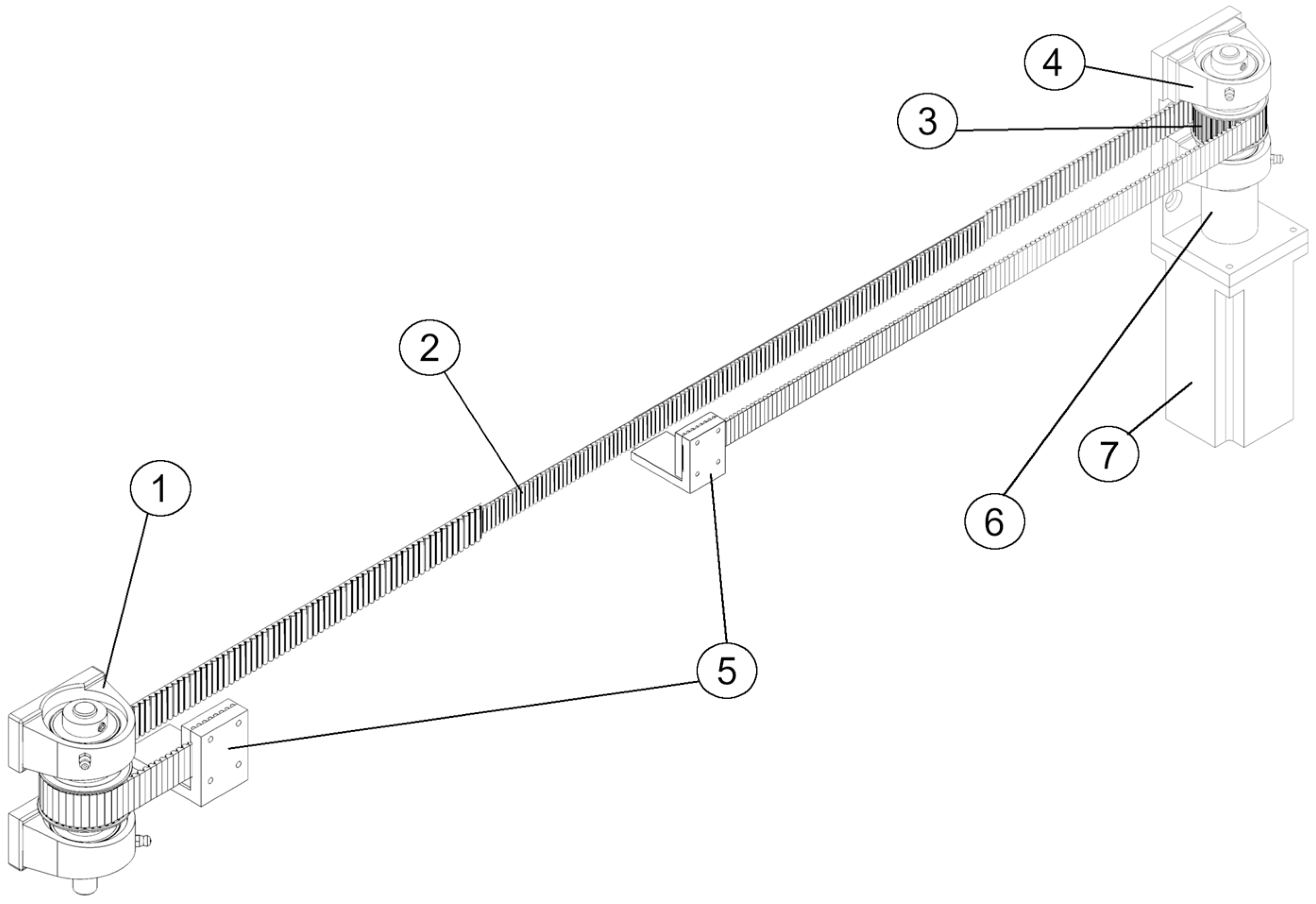
2.1. Stage 1. Selection of Basic Parameters

Like any product, automatic door drive modules are characterized by a number of parameters—load capacity, stroke length, speed, etc., some of which are primary and others secondary. The primary parameters of the product determine its ability to perform a certain number of predetermined functions, and secondary parameters are all the others that are of secondary importance to the product and do not determine the ability of the product to perform its assigned tasks.
The correct determination of the set of primary parameters, in view of which the optimization will be carried out, predetermines to a significant extent the effectiveness of the size range. The complexity and laboriousness of solving the optimization problem also depends on the choice of parameters.
After analyzing the set of product parameters and taking into account the requirement for orthogonality (independence), one primary parameter x l is selected for the product under consideration—the load capacity, which is determined by the mass of the wing. It is an integral parameter, as it is related to both the stroke length and the driving belt (the overall dimensions of the wing), and the power of the motor required for the drive. Therefore, the load capacity of the module determines the most important operational (functional) parameters of the product and has stability. The stability property in this context means that the parameter is independent of frequently changing factors such as production technology, materials used, etc., and does not limit the possibilities for improving the design of the product.
After market research encompassing the Eastern European market for automatic sliding doors and specifically the market share of the mentioned leading manufacturers, the limits of variation of the main parameter are determined:
x ¯ l 223,15 ; 629,99   k g
where x ¯ l , l = 1 ÷ L ¯ , is the load capacity of i -th size, kg; and L ¯ —is the total number of sizes determined from the market research.
The study conducted, based on customer orders for the years 2023–2024, has established that in the considered range there is a demand for L ¯ = 110 module sizes that make up the initial size range.

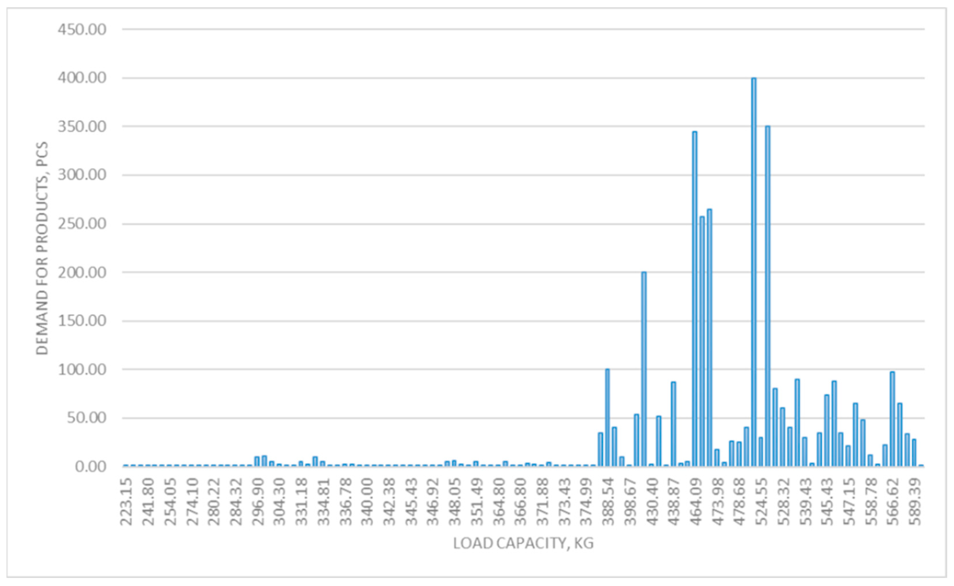
2.2. Stage 2. Determining Demand

The demand for each element x ¯ l , l = 1 ÷ L ¯ , in the initial size range Z ¯ is determined after the market research, i.e., the elements of the set N ¯ = N ¯ 1 , N ¯ 2 , , N ¯ l , , N ¯ L ¯ , l = 1 ÷ L ¯ , are determined, where N ¯ l is the quantity of products with value of the main parameter x ¯ l .
The obtained results for the demand are shown in Figure 3, where the values of the main parameter (the mass of the wing) are plotted on the abscissa, and the corresponding quantity on the ordinate. Additionally, the exact values can be read in Appendix A.

2.3. Stage 3. Selection of Optimality Criterion

To solve the problem, it is proposed to use the total costs of the range, which must be minimized, as a criterion for optimality. They include the costs of manufacturing all sizes in the range, estimated by the cost of the main components of the product, representing the most significant variable part of these costs, and additional costs in the field of operation, which take into account the discrepancy between the required and offered sizes.
In this way, the selected criterion takes into account the conflicting interests of manufacturers and users. It should be noted that the total costs do not include the costs of power and maintenance during the operation of the product. Since the optimization proposed will always reduce the operation costs in respect to an oversized module, this aspect is not considered here, focusing on the costs of production.
Therefore, the selected criterion for evaluating alternative size ranges has the following form:
R = j = 1 L T S ( x l j ) · N l j · N T S N l j ν 1 + j = 1 L u U l j D R ( x l j , x ¯ u , N ¯ u )
where R is the total cost for all elements in the size range; L —the number of elements in the current range Z = { x l 1 ,   x l 2 ,     , x l j ,     , x l L } being analyzed; x l j —the value of the main parameter (the load capacity of the module) of l j -th size in current row; T S ( x l j ) —production costs of l j -th size; N l j —the quantity (number) of l j -th size product; u U l j D R ( x l j , x ¯ u , N ¯ u ) —the additional costs of a mismatch between demand and supply for l j -th size in the current range that replaces sizes x ¯ u , u U l j , elements of the initial size range Z ¯ = { x ¯ 1 ,   x ¯ 2 ,     , x ¯ l ,     , x ¯ L ¯ } , l = 1 ÷ L ¯ ; U l j —the set of element indices in the initial size range that are replaced by l j -th size in the current range; N ¯ u —the quantity (number) of u -th product size, u U l j , elements of the initial size range; v 1 —the coefficient characterizing the intensity of cost changes depending on the change in the production program, taking into account the “learning rate” [27,28]; N T S —the coefficient taking into account the scale factor in the sphere of production and operation of the product.
To calculate the additional costs taking into account the use of oversized modules instead of the necessary ones, the following dependence is proposed:
j = 1 L u U l j D R x l j , x ¯ u , N ¯ u = u = 1 l 1 N ¯ u T S x l 1 T S x ¯ u + α j = 2 L u = l j 1 + 1 l j N ¯ u T S x l j T S x ¯ u
where T S x l 1 is the cost of producing the first size in the current size range; T S x ¯ u —the cost of producing the u -th size from the initial size range; α —Boolean variable, where α = 0 , when L = 1 , i.e., l 1 = L ¯ , and α = 1 when L = 2 ÷ L ¯ . In short, the result of (3) is the cost difference between using exactly the demanded module and using an oversized module.

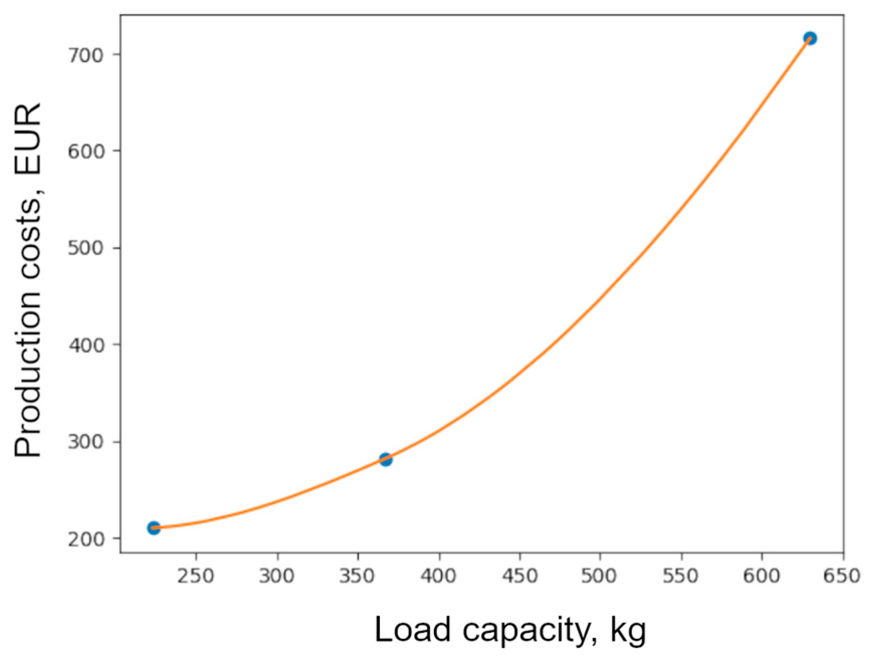
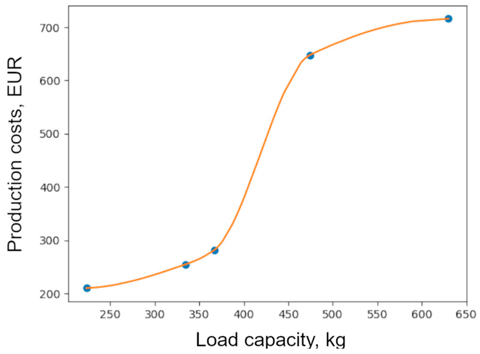
2.4. Stage 4. Development of a Cost Model

Production costs T S ( x l j ) are modeled on the basis of the cost of the building components of the drive modules. The most significant share determining these costs are the following three components: motor, belt, and pulleys. Engineering calculations have been performed to select these components for specific values of the main parameter, load capacity. After calculations for selecting belt drive and motor corresponding to the loading, the components’ prices are obtained from selected suppliers [29,30]. In the following calculations, risk and uncertainty are not considered, i.e., the calculations are under certain conditions and without taking into account risk (chosen concrete suppliers of parts, no change in the economic conditions).
At first, from the initial size range Z ¯ of one hundred and ten sizes, three elements x ¯ 1 , x ¯ 55 , x ¯ 110 are selected. Cost calculations are made for them, and the relevant components have been selected and valued, i.e., T S ( x ¯ 1 ) , T S ( x ¯ 55 ) , and T S ( x ¯ 110 ) are calculated. These sizes are selected on the basis of equal intervals in the size index range l j 1 ; 110 . To determine the cost of the remaining one hundred and seven sizes, a method of piecewise interpolation using a cubic Hermite interpolation polynomial, proposed in [31], was used. The selected interpolation polynomial preserves the monotonicity in the interpolated data and does not skip points if the data do not describe a smooth function.
The result of the interpolation at the three selected points is shown in Figure 4. The values for the load capacity of the modules in kg are plotted on the abscissa, and the production costs in € on the ordinate. The points of the input data are depicted as solid points connected by a curve depicting the interpolation polynomial.
Then, the interpolation polynomial was calculated for data with two added points to the original three from Figure 4, i.e., the cost was calculated for five sizes, and the corresponding polynomial was built on this basis—in this case, the production costs for sizes x ¯ 1 , x ¯ 28 ,   x ¯ 55 , x ¯ 82 , x ¯ 110 . The result is shown in Figure 5.
Comparing the results obtained from Figure 4 and Figure 5, it is evident that there are significant differences; therefore, five more points were added to the calculated five points, x ¯ 1 , x ¯ 14 , x ¯ 28 ,   x ¯ 41 , x ¯ 55 , x ¯ 68 , x ¯ 75 , x ¯ 82 , x ¯ 96 , x ¯ 110 , and the interpolation polynomial was generated again (Figure 6).
Analyzing the results of Figure 5 and Figure 6, some differences in the interpolation polynomial are visible, but to a significant extent it retains its form. The final interpolation polynomial used for the production cost model is given in Figure 7. The difference between it and the one shown in Figure 6 is in one added point, i.e., for Figure 7, x ¯ 1 , x ¯ 14 , x ¯ 28 ,   x ¯ 41 , x ¯ 55 , x ¯ 68 , x ¯ 75 , x ¯ 82 , x ¯ 96 , x ¯ 103 , x ¯ 110 .
A consideration for stopping further addition of interpolation points is the limited variety of motor sizes and belt and pulley sizes available on the market (also subject to size ranges), i.e., differences in production costs upon further granulation would arise from different belt lengths. Since the lengths of the door wings increase relatively smoothly, the change in belt length will have a smaller impact on production costs when comparing adjacent sizes. Therefore, it is considered that the interpolation polynomial depicted in Figure 7 interpolates T S ( x l j ) with sufficient accuracy.
Therefore, the dependence for the total costs has the following form:
R = j = 1 L T S ( x l j ) · N l j · 30 N l j 0.25 + j = 1 L u U l j D R ( x l j , x ¯ u , N ¯ u )
where T S ( x l j ) is determined by the interpolation polynomial, graphically depicted in Figure 7; determining values for T S ( x l j ) at points l = 1 ÷ 110 is specified in Appendix B.
Figure 8 shows the change in the total costs R (set of points 3) and the two components included in them. Each point on the abscissa represents the number of elements in a size range that satisfies all demand with the minimum total cost. This is a graphical representation of the optimal values for the cost components (production and additional costs) and total costs for all possible size ranges of the problem being solved. The graphical representation includes size ranges built from 1 to 110 elements (sizes) ( l = 1 ÷ 110 ). As can be seen from the figure, the objective function (set of points 3) is a discrete convex function and has a global minimum. This property will be used when determining the condition for stopping the calculations according to the selected optimization method.

2.5. Stage 5. Building a Mathematical Model

The problem of selecting an optimal size range of sliding door drive modules is a one-parameter optimization problem in which there are no restrictions on the applicability of the elements constituting the size range. In this case, each element in the evaluated alternative size ranges has a greater value of its main parameter than the value of the previous element in the range.
According to [26], the considered problem is of the first hierarchical level and its mathematical model has the following form:
For a given demand set N ¯ = N ¯ 1 , N ¯ 2 , , N ¯ n , , N ¯ L ¯ , of products Z ¯ = x ¯ 1 , x ¯ 2 , , x ¯ n , , x ¯ L ¯ , x ¯ n 1 < x ¯ n , n = 1 ÷ L ¯ , characterized by one main parameter x ¯ —load capacity of the module, find L * , Z * = x l 1 * , x l 2 * , , x l k * , , x l L * * , Z * Z ¯ , l k 1 , 2 , , L ¯ , N * = N * 1 , N * 2 , , N * k , , N * L * , k = 1 ÷ L * , L * L ¯ , which minimize the chosen optimality criterion:
m i n R L , x ¯ 1 , , x ¯ n , , x ¯ L ¯ , N ¯ 1 , , N ¯ n , , N ¯ L ¯ = j = 1 L G x l j , N j , L = 1 ÷ L ¯
under the following conditions:
j = 1 L N j = k = 1 L * N * k = n = 1 L ¯ N ¯ n = N 0
x l L = x l L * * = x ¯ L ¯
x l j Z ¯ = x ¯ 1 , x ¯ 2 , , x ¯ l , , x ¯ m , , x ¯ L ¯ , j = 1 ÷ L ¯
x l j 1 < x l j , j = 1 ÷ L
where L ¯ is the number of elements in the initial size range Z ¯ = x ¯ 1 , x ¯ 2 , , x ¯ l , , x ¯ m , , x ¯ L ¯ , determined after a demand study; L —the number of elements in the currently analysed range Z = x l 1 , x l 2 , , x l j , , x l L , l j 1 , 2 , , L ¯ . There is a unique mapping between the elements in the current and initial range, where each element x l j matches with one element x ¯ m . The elements of the current ranges are a combination of L , L = 1 ÷ L ¯ , elements of possible L ¯ number of elements of the initial size range; L * —the number of elements in the optimal size range Z * = x l 1 * , x l 2 * , , x l k * , , x l L * * , k = 1 ÷ L * , L * L ¯ ; N j —demand for product x l j element of the currently analysed range Z = x l 1 , x l 2 , , x l j , , x l L , which index l j corresponds to the index m of product x ¯ m Z ¯ , element of the initial size range, as x l j = x ¯ m , N j = p = l + 1 m N ¯ p , and x l j 1 = x ¯ l , m , l 1 , 2 , , L ¯ ; N * k —the number of products from l k -th size in the optimal size range; N 0 —the total quantity of product demand; N ¯ = N ¯ 1 , N ¯ 2 , , N ¯ n , , N ¯ L ¯ , n = 1 ÷ L ¯ —the set of product demand of the initial size range, which is specified in a tabular form.
Condition (6) means that all analyzed ranges, including the optimal one, must satisfy all demand; condition (7) means that in each size range, including the optimal one, the element from the initial range with the maximum values of its main parameter x ¯ L ¯ must be included; and condition (8) that the elements of all ranges are selected from the set of elements of the initial row, determined after studying the demand. Condition (9) means that each element in the evaluated alternative size ranges has a greater value of its main parameter than the value of the previous element of the range.

2.6. Stage 6. Selection of a Mathematical Method

The formulated problem is characterized by a large number of possible size ranges that must be analyzed. This number is determined by the dependence k = 1 L ¯ 1 C L ¯ 1 k = 2 L ¯ 1 1 , where k is the number of elements in the range formed by elements of the initial size range with L ¯ elements [8].
For the considered problem, L ¯ = 110 . Therefore, the number of alternative size ranges is 2 109 1 = 6.4903711 × 1 0 32 1 . The time involved to solve the problem with 7 elements in the size range is about 137 min (Intel Core i7-4710HQ CPU, 2.50 GHz, 8 GB RAM). A conservative (polynomial) estimation of the calculation time for L ¯ = 110 is about 339 years. The time involved makes it impossible to solve the problem by full combination and necessitates the use of a method for directed search for the optimal solution.
One of the effective methods for solving the formulated problem is the dynamic programming method [32], which will be applied in this paper. The main advantage of the method is its good adaptability for solving discrete optimization problems, as its application does not depend on the type of objective function.
According to the chosen method, the following recurrent dependencies for determining the total costs have been derived: for l = 1 , m = l ÷ L ¯ ,
R m 1 = G x ¯ m , p = 1 m N ¯ p = T S x ¯ m · p = 1 m N ¯ p ·   N T S p = 1 m N ¯ p ν 1 + p = 1 m D R x ¯ m , x ¯ p , p = 1 m N ¯ p
for l = 2 ÷ L ¯ , m = l ÷ L ¯ , m ¯ ~ = ( l 1 ) ÷ ( m 1 ) ,
R m l = min R m ¯ ~ l 1 + G x ¯ m , p = m ¯ ~ + 1 m N ¯ p   = R m ¯ ~ l 1 + T S x ¯ m · p = m ¯ ~ + 1 m N ¯ p ·   N T S p = m ¯ ~ + 1 m N ¯ p ν 1 + p = m ¯ ~ + 1 m D R x ¯ m , x ¯ p , p = m ¯ ~ + 1 m N ¯ p
where R m l is the minimum (optimal) value of the objective function to satisfy the demand for products with values of the main parameter in the interval ( 0 , x ¯ m ] , m = 1 ÷ L ¯ , with l number of sizes; L ¯ —the number of permissible values of the main parameter of the product; N ¯ p —the demand for products with values of the main parameter in the range ( x ¯ p 1 ,   x ¯ p ] .
Since the objective function is a discrete convex function and has a global minimum, the calculation of R m l , l = 1 ÷ L ¯ , continues until the following condition is met:
R L ¯ l R L ¯ l + 1

2.7. Stage 7. Algorithmic and Software Support

Two algorithms are developed to solve the problem—the first implementing a full combination method taking into account the additional costs due to discrepancy, which will be used to solve problems with a small number of possible size ranges and to verify the results of the application of the dynamic programming method, and the second implementing the proposed recurrent dependencies (10) and (11) and condition (12).

2.7.1. Full Combination Algorithm

The complete algorithm can be read in Appendix C.1. Here, the main structure is discussed.
The necessary input data for the algorithm are the values of the main parameter x ¯ n for each element of the initial size range Z ¯ , and the demand N ¯ n for each element x ¯ n , n = 1 ÷ L ¯ .
The algorithm iterates over all combinations without repetition of l elements from L ¯ , l = 2 ÷ L ¯ , i.e., C L ¯ l . The first iteration is for the special case of l = 1 . This is a special case, because the number of possible size ranges is 1, and not C L ¯ 1 . This case coincides with the size range composed of only the biggest (in terms of value of the main parameter) element x ¯ L ¯ . Next, iterations generate size ranges with number of elements l = 2 ÷ L ¯ . For l = 2 , there are C L ¯ 2 number of size ranges (combinations of elements x ¯ n ), for l = 3 , there are C L ¯ 3 number of size ranges, etc. For each of these size ranges, the following calculations are made in this sequence: calculate demand for each element in the current (current combination of elements) size range; calculate production costs j = 1 L T S ( x l j ) · N l j · N T S N l j ν 1 ; calculate additional costs j = 1 L u U l j D R ( x l j , x ¯ u , N ¯ u ) ; calculate total cost R . After calculating the total cost for the current size range, it is compared to the minimum value of R found so far. If total cost for the current size range is lower than the minimum, then it becomes the current global optimum (minimum); otherwise, iterations continue with the next size range. Additionally, the algorithm searches for local optima, i.e., the size range with min R for the combination set C L ¯ l for a particular l , l = 2 ÷ L ¯ . For example, the local optimum for the combination set C L ¯ 2 is the size range Z = x ¯ l 1 , x ¯ l 2 , l 1 , l 2 1 ÷ L ¯ , which has minimum total cost in comparison to all size ranges with 2 elements that are a combination without repetition from L ¯ . The local optimum for C L ¯ 1 is the size range Z = x ¯ L ¯ , as it is the only possible one in this combination set.
After determining if the current size range is globally, locally, or not optimal, the algorithm generates the next combination (next size range) of elements. The algorithm finishes after all combinations are checked, i.e., after 2 L ¯ 1 1 iterations.

2.7.2. Algorithm Implementing the Dynamic Programming Method

The complete algorithm can be read in Appendix C.2. Here, the main structure is discussed.
The necessary input data for the algorithm are the values of the main parameter x ¯ n for each element of the initial size range Z ¯ , and the demand N ¯ n for each element x ¯ n , n = 1 ÷ L ¯ .
The algorithm uses previously calculated cost values for accelerating the finding of optima. These costs are remembered in an upper triangular matrix C L ¯ × L ¯ . In the beginning the total costs R m 1 of each element (size) x ¯ m , m = 1 ÷ L ¯ , is calculated from (10). These costs form the first row of C L ¯ × L ¯ . Cost calculations continue using the expression (11) for R m l , l = 2 ÷ L ¯ , m = l ÷ L ¯ where R m l is the minimum (optimal) value of the objective function to satisfy the demand for products with values of the main parameter in the interval ( 0 , x ¯ m ] , m = 1 ÷ L ¯ , with l number of sizes. In (11), the term R m ¯ ~ l 1 , m ¯ ~ = ( l 1 ) ÷ ( m 1 ) , refers to costs that have been previously calculated and remembered in C L ¯ × L ¯ , where l 1 indicates the row from which the cost value is taken and m ¯ ~ —the column. The last column of the table C L ¯ × L ¯ yields the optima for the size ranges with number of elements corresponding to the row index. Thus, C 2 × L ¯ is the optimum for the size ranges with 2 elements from L ¯ . The optimal total cost is found by selecting the minimum value of the values in the last column of table C L ¯ × L ¯ . The algorithm stops after calculating all values in the table and selecting the minimum total cost from the L ¯ -th column.

2.7.3. Software Applications

Software applications using the proposed algorithms are developed. The application implementing the full combination algorithm outputs a text file with data about the found optimum for size ranges with an increasing number of elements, i.e., for L = 1 ÷ L ¯ (Figure 9). Additional information about the elements in the optimal range, the total costs, and the time to reach this solution is also output.
Implementation of the software applications is done in C++ programming language. These are command line interface executables which operate with a simple textual input file including data regarding the number of sizes in the initial size range, list of values of the main parameter, and list of values for the demand corresponding to each parameter value. No third-party libraries are used. Verifying the correct working of the developed software applications is done through solving test problems from specialized literature.
The application implementing the dynamic programming algorithm saves the data from solving the problem in a CSV file. The file can then be opened in a program that allows working with CSV files.

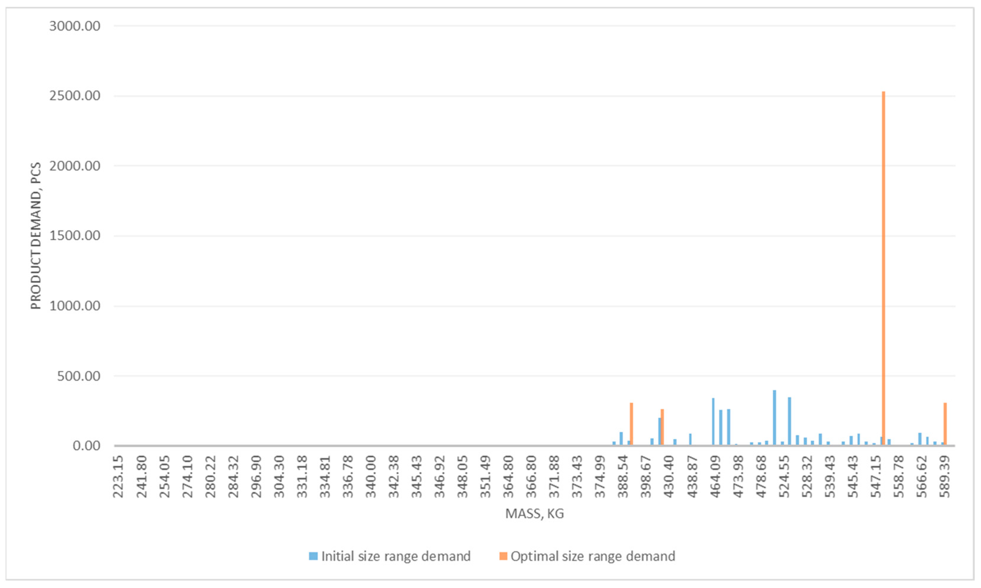
2.8. Stage 8. Solving the Problem—Choosing the Optimal Size Range

The problem (5)–(9) is solved using the developed tools (mathematical model of the optimization problem, model of the total costs, algorithms, and application programs).
The results are shown in Table 1, where R * is the minimum (optimal) total costs, €; L * —the number of elements in the optimal size range; R L ¯ L ¯ —the total costs for the size range including all sizes, i.e., the initial size range, €.
Table 2 shows the data for the chosen optimal size range, which includes L * = 5 elements. Each element satisfies demand in the range from the previous element until the current element in the range, i.e., x ¯ 68 satisfies the demand for sizes from x ¯ 1 to x ¯ 68 inclusive, x ¯ 72 satisfies the demand for sizes from x ¯ 69 to x ¯ 72 inclusive, etc.
Figure 10 shows the demand of the elements of the optimal size range and the elements of the initial size range, and Figure 11—the total costs determined in the process of solving the problem as a discrete function, with an approximating polynomial of the sixth degree. Each point on the abscissa of Figure 11 represents the number of elements in a size range that satisfies all demand with minimum total cost, i.e., minimum total costs for a size range with 1 size, with 2 sizes, etc.
The optimal solution found has the following characteristics:
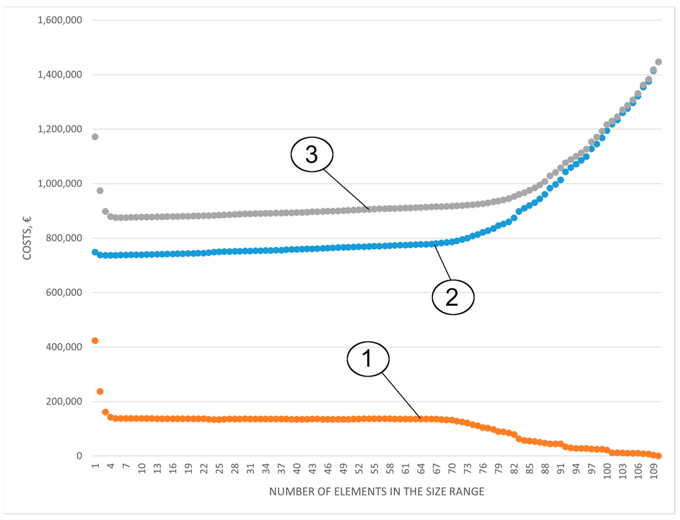
  • Reduction of the number of sizes from 110 to 5, i.e., by approximately 96%;
  • Reduction of total costs compared to the size range including all possible sizes by €571,317.56, or by 39.5%;
  • Reduction of total costs compared to a range including only one (largest) size by 34%, which is the most common case in practice.

2.9. Stage 9. Studying the Sensitivity of the Optimal Solution

A study and analysis of the sensitivity of the found optimal solution to the problem is carried out. For this purpose, the problem is solved by changing one or several parameters of the mathematical model within certain limits while maintaining the value of the others. The main goal is to determine the influence of these parameters on the solution of the optimization problem and determine the most important ones for which the most accurate information should be obtained.
For this purpose, in [33] numerical experiments have been conducted, which consist of solving the problems (5)–(9) at different values of the main coefficients and components included in the mathematical model.
The sensitivity analysis includes the following experiments:
A. Changing the demand set N ¯ = N ¯ 1 , N ¯ 2 , , N ¯ n , , N ¯ L ¯ while maintaining the total produced quantity N 0 ;
B. Changing the production program N 0 ;
C. Changing the coefficient taking into account the scale of production N T S ;
D. Changing the coefficient taking into account the learning rate ν 1 .
As a result of the conducted numerical experiments, the following findings are made:
  • The demand function, the coefficients taking into account the scale of production, and the learning rate must be determined as accurately as possible, since they have a significant impact on the optimal solution;
  • Changing the production program does not have a significant impact on the number and type of elements in the optimal size range, as its change leads only to a change in the amount of total costs.

3. Conclusions

In this work, an approach for optimizing size ranges of technical products is tested, using the example of a module for driving automatic sliding doors, and the following important results have been achieved:
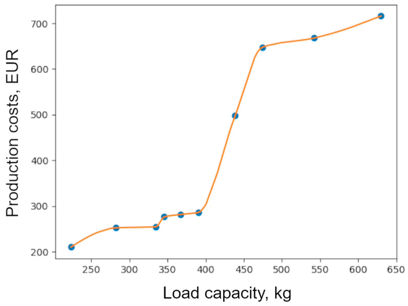
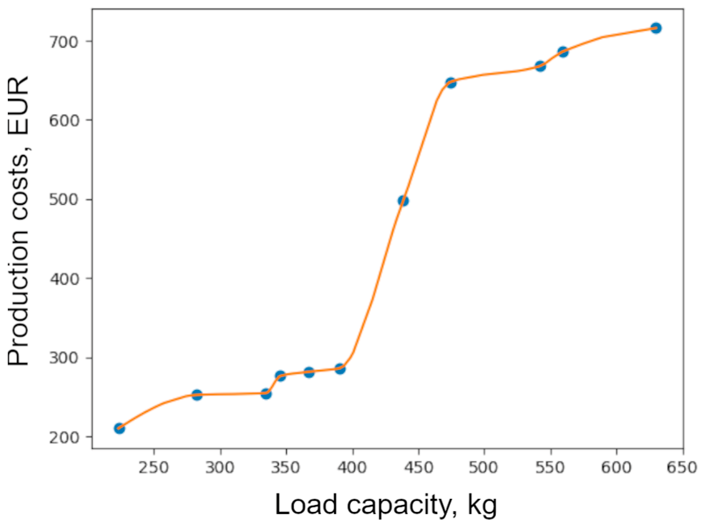
  • The demand for modules for driving automatic sliding doors is determined as a function of their load capacity.
  • A mathematical model of the problem for choosing an optimal size range is developed.
  • The analytical dependence of the optimality criterion “total costs” is proposed, including the main variable production costs and additional costs in the field of operation, which take into account the discrepancy between the required and offered standard sizes.
  • The functional dependence between the total costs and the influencing parameters has been determined using an established interpolation method.
  • Recurrence relations for calculating the total costs based on the Bellman optimality principle have been derived.
  • Algorithms and the corresponding software applications have been developed to solve the problem.
  • The optimal size range of modules for driving automatic sliding doors is determined, which is characterized by a reduction in the number of elements in the initial range, determined after the market research, by 96%; a reduction in total costs compared to the initial range by 39.5%; and with the range including only the largest size, which is the most common case in practice, by 34%.
In addition to the achieved goal—choosing of an optimal size range of modules for driving automatic sliding doors—this work proves the applicability of the approach used, which due to its universal nature can be applied to the optimization of size ranges of other products after building the relevant demand and cost models, and adapting it to the conditions of the specific problem.
Future research will be aimed at solving multiparametric optimization problems for size range optimization; problems with constraints on the applicability of the different sizes (application ranges); and studying different ways of building size ranges and improving known software products for designing and creating technical documentation for automatic sliding doors based on the developed size range of the drive system.

Author Contributions

I.M., V.Z. and H.H. were involved in the full process of producing this paper, including conceptualization, methodology, modeling, validation, visualization, and preparing the manuscript. All authors have read and agreed to the published version of the manuscript.

Funding

This research was funded by the European Union—Next Generation EU, project № BG-RRP-2.004-0005.

Data Availability Statement

Data are contained within the article.

Acknowledgments

This study is financed by the European Union—Next Generation EU, through the National Recovery and Resilience Plan of the Republic of Bulgaria, project № BG-RRP-2.004-0005.

Conflicts of Interest

The authors declare no conflicts of interest.

Appendix A

The demand N ¯ l for each element x ¯ l , l = 1 ÷ L ¯ , in the initial size range Z ¯ , is given as a tuple ( x l ; N ¯ l ), i.e., (main parameter value [kg], demand value [pcs]), in the following set: {(223.15; 1), (234.22; 1), (236.65; 1), (241.80; 1), (244.36; 1), (250.82; 1), (254.05; 1), (257.28; 1), (257.93; 1), (274.10; 1), (276.14; 1), (278.17; 1), (280.22; 1), (282.60; 1), (283.98; 1), (284.32; 1), (287.04; 1), (287.72; 1), (296.90; 10), (299.01; 11), (303.96; 5), (304.30; 2), (306.79; 1), (310.29; 1), (331.18; 5), (334.14; 2), (334.51; 10), (334.81; 5), (335.64; 1), (335.72; 1), (336.78; 2), (337.92; 2), (339.41; 1), (340.00; 1), (340.89; 1), (341.64; 1), (342.38; 1), (344.68; 1), (345.06; 1), (345.43; 1), (345.80; 1), (346.55; 1), (346.92; 1), (347.30; 1), (347.83; 5), (348.05; 6), (348.83; 2), (349.58; 1), (351.49; 5), (355.25; 1), (364.34; 1), (364.80; 1), (365.11; 5), (366.03; 1), (366.80; 1), (367.88; 3), (371.49; 2), (371.88; 1), (372.66; 4), (373.04; 1), (373.43; 1), (374.21; 1), (374.60; 1), (374.99; 1), (376.58; 1), (387.00; 35), (388.54; 100), (390.40; 40), (393.76; 10), (398.67; 1), (400.92; 54), (415.42; 200), (430.40; 2), (433.36; 52), (438.62; 1), (438.87; 87), (442.77; 3), (445.38; 5), (464.09; 345), (468.23; 257), (473.09; 265), (473.98; 18), (474.88; 4), (478.41; 26), (478.68; 25), (480.62; 40), (498.80; 400), (524.55; 30), (525.96; 350), (527.38; 80), (528.32; 60), (529.27; 40), (532.29; 90), (539.43; 30), (541.33; 3), (541.81; 35), (545.43; 74), (546.38; 88), (546.39; 35), (547.15; 21), (547.34; 65), (551.15; 48), (558.78; 12), (559.73; 2), (563.37; 22), (566.62; 97), (570.62; 65), (575.80; 34), (589.39; 28), (629.99; 1)}.

Appendix B

The values for T S ( x l j ) , EUR, at points l = 1 ÷ 110 specified in the following set: {209.99, 221.5, 223.91, 228.86, 231.2, 236.75, 239.28, 241.64, 242.1, 250.46, 251.07, 251.57, 251.95, 252.24, 252.35, 252.38, 252.57, 252.61, 253.01, 253.07, 253.18, 253.19, 253.24, 253.31, 254.31, 254.61, 254.66, 254.69, 255.09, 255.16, 256.53, 258.76, 262.48, 264.09, 266.56, 268.62, 270.54, 275.13, 275.6, 275.94, 276.18, 276.53, 276.69, 276.86, 277.07, 277.16, 277.46, 277.73, 278.33, 279.27, 280.91, 281.0, 281.06, 281.24, 281.4, 281.62, 282.26, 282.32, 282.44, 282.5, 282.56, 282.67, 282.73, 282.78, 283.01, 284.89, 285.3, 285.87, 288.83, 299.21, 306.07, 372.65, 457.15, 472.67, 497.5, 498.58, 516.89, 530.27, 624.32, 637.81, 646.81, 647.51, 648.05, 649.99, 650.12, 651.05, 656.73, 661.42, 661.77, 662.14, 662.4, 662.68, 663.64, 666.52, 667.46, 667.71, 670.6, 671.62, 671.62, 672.51, 672.73, 677.58, 685.81, 686.44, 688.84, 690.96, 693.51, 696.71, 704.36, 715.97}.

Appendix C

Appendix C.1

Algorithm A1: Full combination algorithm
  Step 1. Entering input information: Z ¯ = x ¯ 1 , x ¯ 2 , , x ¯ n , , x ¯ L ¯ , N ¯ = N ¯ 1 , N ¯ 2 , , N ¯ n , , N ¯ L ¯ , n = 1 ÷ L ¯ . The following sets are defined: the set I = i 1 , i 2 , , i η , , i L ¯ , i 1 = L ¯ , which is used to store the indices of the current combination of elements in the currently analyzed size range; the set N = N 1 , N 2 , , N n , , N L ¯ , which is used to calculate the element demand for the currently analyzed size range, N n = 0 , n = 1 ÷ L ¯ .
  Step 2. j = 1 . If j L ¯ follows Step 3, otherwise follows Step 61.
  (Step 3 to Step 6—generate first combination of element indices for current size ranges containing number of elements  j )
  Step 3. k = 2 .
  Step 4. If k j follows Step 5, otherwise follows Step 7.
  Step 5. i k = L ¯ k + 1 .
  Step 6. k = k + 1 . Follows Step 4.
  Step 7. R j * = 0 .
  (Step 8 to Step 22—calculating the demand of the elements that make up the current size range)
  Step 8. If j > 1 follows Step 9, otherwise follows Step 19.
  Step 9.  k = 1 .
  Step 10. If k < j follows Step 11, otherwise follows Step 16.
  Step 11.  m = i k .
  Step 12. If m > i k + 1 follows Step 13, otherwise follows Step 15.
  Step 13. N k = N k + N ¯ m .
  Step 14.  m = m 1 . Follows Step 12.
  Step 15. k = k + 1 . Follows Step 10.
  Step 16. If m > 0 follows Step 17, otherwise follows Step 23.
  Step 17.  N k = N k + N ¯ m .
  Step 18.  m = m 1 . Follows Step 16.
  Step 19.  k = 1 .
  Step 20. If k L ¯ follows Step 21, otherwise follows Step 23.
  Step 21.  N 1 = N 1 + N ¯ k .
  Step 22. k = k + 1 . Follows Step 20.
  (Step 23 to Step 26—calculation of production costs  T S of the current size range)
  Step 23. k = 1 , T S = 0 .
  Step 24. If k j follows Step 25, otherwise follows Step 27.
  Step 25.  T S = T S + T S x ¯ i k N k 30 N k 0.25 .
  Step 26. k = k + 1 . Follows Step 24.
  (Step 27 to Step 37—calculation of additional costs  D R of the current size range)
  Step 27. k = 1 , D R = 0 .
  Step 28. If k < j follows Step 29, otherwise follows Step 34.
  Step 29. m = i k 1 .
  Step 30. If m > i k + 1 follows Step 31, otherwise follows Step 33.
  Step 31. D R = D R + N m T S x ¯ i k T S x ¯ m .
  Step 32. m = m 1 . Follows Step 30.
  Step 33. k = k + 1 . Follows Step 28.
  Step 34. m = i j .
  Step 35. If m > 0 follows Step 36, otherwise follows Step 38.
  Step 36. D R = D R + N m T S x ¯ i j T S x ¯ m .
  Step 37. m = m 1 . Follows Step 35.
  (Step 38—calculate the total cost  R for the current size range)
  Step 38. R = T S + D R .
  (Step 39 to Step 41—checking for global optimum)
  Step 39. If j > 1 follows Step 40, otherwise follows Step 41.
  Step 40. If o p t R > R follows Step 41, otherwise follows Step 42.
  Step 41.  o p t R = R . The indices i η from the set I for which η 1 ; j is satisfied are stored in the set I * , which contains the indices of the elements of the optimal size range. If from previous iterations of the algorithm the set I * contains indices, then its elements are completely replaced by the elements i η , η 1 ; j .
  (Step 42 to Step 44—checking for local optimum, i.e., for the set of size ranges with the same number of sizes  j )
  Step 42. If R j * > 0 follows Step 43, otherwise follows Step 44.
  Step 43. If R j * > R , follows Step 44, otherwise follows Step 45.
  Step 44. R j * = R .
  (Step 45 to Step 58—generate next combination of element indices for next current size range)
  Step 45.  k = j , m = 1 .
  Step 46. If k > 1 follows Step 47, otherwise follows Step 49.
  Step 47. If i k m follows Step 49, otherwise follows Step 48.
  Step 48.  k = k 1 , m = m + 1 . Follows Step 46.
  Step 49. If k = 1 follows Step 60, otherwise follows Step 50.
  Step 50.  k = j .
  Step 51. If k > 1 follows Step 52, otherwise follows Step 55.
  Step 52. If i k j k follows Step 53, otherwise follows Step 54.
  Step 53.  i k = i k 1 . Follows Step 55.
  Step 54.  k = k 1 . Follows Step 51.
  Step 55. m = k + 1 p = 1 .
  Step 56. If m < j + 1 follows Step 57, otherwise follows Step 59.
  Step 57. i m = i k p .
  Step 58. m = m + 1 p = p + 1 . Follows Step 56.
  Step 59. N n = 0 , n = 1 ÷ L ¯ . Follows Step 8.
  Step 60. N n = 0 , n = 1 ÷ L ¯ . At this stage in o p t R , R j * and I * are recorded, respectively, the optimal value for the total costs found up to the current iteration of the algorithm, the optimal value for the total costs for size ranges with j number of elements and the indices of the elements constituting the size range with total costs o p t R . Follows Step 2.
  Step 61. The optimum for total costs is o p t R , and the elements of the optimal size range are I * . End.

Appendix C.2

Algorithm A2: Algorithm implementing the dynamic programming method
  Step 1. Entering input information: Z ¯ = x ¯ 1 , x ¯ 2 , , x ¯ n , , x ¯ L ¯ , N ¯ = N ¯ 1 , N ¯ 2 , , N ¯ n , , N ¯ L ¯ , n = 1 ÷ L ¯ . The following matrices are defined: of the minimum costs C L ¯ × L ¯ = c m p , c m p = , and the indices of the elements (sizes) that participate in the size ranges with minimum costs I L ¯ × L ¯ = i m p , i m p = 0 .
  Step 2.  m = 1 , l = 1 .
  Step 3. Calculating R m 1 = G x ¯ m , p = 1 m N ¯ p , after which c m 1 = R m 1 .
  Step 4.  m = m + 1 . If m > L ¯ follows Step 5, otherwise return to Step 3.
  Step 5. l = 2 . If  l > L ¯ follows Step 12, otherwise follows Step 6.
  Step 6.  m = 1 .
  Step 7.  m ¯ ~ = l 1 .
  Step 8. Calculating R m l = c m ¯ ~ l 1 + G x ¯ m , p = m ¯ ~ + 1 m N ¯ p . If c m l > R m l , then c m l = R m l and i m l = m ¯ ~ .
  Step 9.  m ¯ ~ = m ¯ ~ + 1 . If m ¯ ~ > m 1 follows Step 10, otherwise follows Step 8.
  Step 10.  m = m + 1 . If m > L ¯ follows Step 11, otherwise follows Step 7.
  Step 11.  l = l + 1 . If l > L ¯ follows Step 12, otherwise follows Step 6.
  Step 12.  o p t R = , L * = 0 , l = 1 .
  Step 13. If o p t R > c L ¯ l , then o p t R = c L ¯ l and L * = l .
  Step 14.  l = l + 1 . If l > L ¯ follows Step 15, otherwise follows Step 13.
  Step 15. The optimal size range having total costs o p t R , is Z * = x l 1 * , x l 2 * , , x l k * , , x l L * * , N * = N * l 1 , N * l 2 , , N * l k , , N * l L * . The indices of its members, elements of the initial size range, are determined by the matrix I L ¯ × L ¯ = i m p , starting from the last to the first: l L * = L ¯ , l k = i k + 1 k + 1 , where k = L * 1 ÷ 1 . End.

References

  1. Dormakaba. Meeting All Your Access Needs; Product Brochure; Dormakaba: Rümlang, Swithzerland, 2022. [Google Scholar]
  2. Alumil. Available online: https://www.alumil.com/international/aluminium-systems/all-architectural-aluminium-systems/minimal-sliding-insulated-system-supreme-s650-phos (accessed on 5 March 2025).
  3. Record. Available online: https://record-bg.com/ (accessed on 5 March 2025).
  4. GEZE. Available online: https://www.geze.com/en/products-solutions/sliding_doors/automatic_sliding_doors/slimdrive/c_36770 (accessed on 5 March 2025).
  5. Pahl, G.; Beitz, W. Konstruktionslehre. Methoden und Anwendung; Springer: Berlin/Heidelberg, Germany, 2007. [Google Scholar]
  6. Vietor, T.; Stechert, C. Produktarten zur Rationalisierung des Entwicklungsund Konstruktionsprozesses. In Pahl/Beitz Konstruktionslehre; Feldhusen, V.J.H., Grote, K.-H., Eds.; Springer: Berlin, Germany, 2013; pp. 817–871. [Google Scholar]
  7. Mueller, D. A cost calculation model for the optimal design of size ranges. J. Eng. Des. 2011, 22, 467–485. [Google Scholar] [CrossRef]
  8. Dashenko, A.; Belousov, A. Design of Automated Lines; Graduate School: Moscow, Russia, 1983. (In Russian) [Google Scholar]
  9. Zhang, M.; Tseng, M. A product and process modeling based approach to study cost implications of product variety in mass customization. IEEE Trans. Eng. Manag. 2007, 54, 130–144. [Google Scholar] [CrossRef]
  10. Zaharinov, V.; Malakov, I.; Hasansabri, H. Choosing of an Optimal Structural Variant of a Basic Size of a Size Range of Modules. Ann. DAAAM Proc. Int. DAAAM Symp. 2023, 34, 62–71. [Google Scholar]
  11. Dichev, D.; Kogia, F.; Koev, H.; Diakov, D. Method of Analysis and correction of the Error from Nonlinearity of the Measurement Instruments. J. Eng. Sci. Technol. Rev. 2016, 9, 116–121. [Google Scholar] [CrossRef]
  12. Dichev, D.; Zhelezarov, I.; Dicheva, R.; Diakov, D.; Nikolova, H.; Cvetanov, G. Algorithm for estimation and correction of dynamic errors. In Proceedings of the 30th International Scientific Symposium Metrology and Metrology Assurance, Sozopol, Bulgaria, 7–11 September 2020. [Google Scholar] [CrossRef]
  13. Kamberov, K.; Todorov, G.; Zlatev, B. Virtual Prototyping-Based Development of Stepper Motor Design. Actuators 2024, 13, 512. [Google Scholar] [CrossRef]
  14. Mitev, P. Development of a Training Station for the Orientation of Dice Parts with Machine Vision. Eng. Proc. 2024, 70, 57. [Google Scholar] [CrossRef]
  15. Nikolov, S.; Dimitrova, R.; Tsolov, S.; Dimitrov, L. Classification of Parallel Kinematics Robots. AIP Conf. Proc. 2024, 3063, 060001. [Google Scholar] [CrossRef]
  16. Todorov, G.; Kralov, I.; Kamberov, K.; Zahariev, E.; Sofronov, Y.; Zlatev, Z. An Assessment of the Embedding of Francis Turbines for Pumped Hydraulic Energy Storage. Water 2024, 16, 2252. [Google Scholar] [CrossRef]
  17. Simpson, T.W. Product platform design and customization. Artif. Intell. Eng. Des. Anal. Manuf. 2004, 18, 3–20. [Google Scholar] [CrossRef]
  18. Ginsburg, A.; Börjesson, F.; Erixon, G. Size ranges in modular products—A financial approach. In Proceedings of the 7th Workshop on Product Structuring–Product Platform Development, Göteborg, Sweden, 24–25 March 2004; pp. 141–150. [Google Scholar]
  19. Lotz, J.; Freund, T.; Würtenberger, J.; Kloberdanz, H. Uncertainty in size range development—An analysis of potential for a new scaling approach. Proc. Int. Des. Conf. 2016, 84, 341–350. [Google Scholar]
  20. Chaymae, B.; Abdellah, E.B. Reconfigurable Manufacturing Systems: Enhancing Efficiency via Product Family Optimization. J. Manuf. Mater. Process. 2025, 9, 39. [Google Scholar] [CrossRef]
  21. Cetin, O.; Saitou, K. Decomposition-based assembly synthesis for structural modularity. ASME J. Mech. Des. 2003, 126, 234–243. [Google Scholar] [CrossRef]
  22. Kipp, T.; Krause, D. Computer aided size range development–data mining vs. optimization. In Proceedings of the ICED 09, the 17th International Conference on Engineering Design, Vol. 4, Product and Systems Design, Palo Alto, CA, USA, 24–27 August 2009; Design Society: Glasgow, UK, 2009; pp. 179–190. [Google Scholar]
  23. Lotz, J. Beherrschung von Unsicherheit in der Baureihenentwicklung. Ph.D. Thesis, TU Darmstadt, Darmstadt, Germany, 2018. [Google Scholar]
  24. Kokkolaras, M.; Fellini, R.; Kim, H.; Michelena, N.; Papalambros, P. Extension of the target cascading formulation to the design of product families. Struct. Multidiscipilnary Optim. 2002, 24, 293–301. [Google Scholar] [CrossRef]
  25. Yu, T.; Yassine, A.A.; Goldberg, D.E. A Genetic Algorithm for Developing Modular Product Architectures. In Proceedings of the ASME 2003 International Design Engineering Technical Conferences and Computers and Information in Engineering Conference. Volume 3b: 15th International Conference on Design Theory and Methodology, Chicago, IL, USA, 2–6 September 2003; pp. 515–524. [Google Scholar] [CrossRef]
  26. Malakov, I.; Zaharinov, V.; Tzenov, V. Size ranges optimization. Procedia Eng. 2015, 100, 791–800. [Google Scholar] [CrossRef]
  27. Groover, M. Automation, Production Systems and Computer-Integrated Manufacturing, 2nd ed.; Prentice Hall: Hoboken, NJ, USA, 2001; ISBN 9780130889782. [Google Scholar]
  28. Du, Z.; Li, J.; Li, J. Hybrid Multi-Objective Artificial Bee Colony for Flexible Assembly Job Shop with Learning Effect. Mathematics 2025, 13, 472. [Google Scholar] [CrossRef]
  29. Mädler Catalogue 43, Catalogue, 1 ed., Mädler. 2025. Available online: https://blaetterkatalog.maedler.de/blaetterkatalog/index.html?catalog=MAEDLER_Katalog43_EN&lang=en#page_1 (accessed on 6 April 2025).
  30. Exoror. Available online: https://www.exoror.com/ (accessed on 6 April 2025).
  31. Fritsch, F.N.; Butland, J. A method for constructing local monotone piecewise cubic interpolants. SIAM J. Sci. Comput. 1984, 5, 300–304. [Google Scholar] [CrossRef]
  32. Bellman, R. Dynamic Programming; Princeton University Press: New York, NY, USA, 1957. [Google Scholar]
  33. Zaharinov, V.; Malakov, I.; Hasansabri, H. Determining the Influence of Model Parameters on the Choosing of an Optimal Size Range of Linear Modules for Automated Sliding Doors. In Proceedings of the 2024 XXXIV International Scientific Symposium Metrology and Metrology Assurance (MMA), Sozopol, Bulgaria, 7–11 September 2024; pp. 1–6. [Google Scholar]
Figure 1. Drive module integrated into the door side pillars.
Algorithms 18 00248 g001
Figure 2. Basic size of a module for driving automatic sliding doors with component designations: 1—Left bearing support; 2—Toothed belt; 3—Driving pulley; 4—Right bearing support; 5—Toothed belt attachment clamps; 6—Coupling; 7—Stepper motor.
Algorithms 18 00248 g002
Figure 3. Product demand determined through market research.
Algorithms 18 00248 g003
Figure 4. Interpolated production cost data at three calculated points.
Algorithms 18 00248 g004
Figure 5. Interpolated production cost data at five calculated points.
Algorithms 18 00248 g005
Figure 6. Interpolated production cost data at ten calculated points.
Algorithms 18 00248 g006
Figure 7. Interpolated production cost data at eleven calculated points.
Algorithms 18 00248 g007
Figure 8. Change in total costs R , where 1—additional costs, u U l j D R ( x l j , x ¯ u , N ¯ u ) ; 2—production costs, T S ( x l j ) · N l j · 30 N l j 0.25 ; 3—total costs, R .
Algorithms 18 00248 g008
Figure 9. Output from the application implementing the full combination algorithm.
Algorithms 18 00248 g009
Figure 10. Demand for the elements of the optimal size range (orange), compared to that of the initial size range (blue).
Algorithms 18 00248 g010
Figure 11. Change in total costs R .
Algorithms 18 00248 g011
Table 1. Results of solving the problem.
IndicatorOptimal Size Range
R * , €875,069, 19
L * 5
R L ¯ L ¯ , €1,446,386, 75
100 R L ¯ L ¯ R * R L ¯ L ¯ , %39.5%
Table 2. Optimal size range.
NoSize
x l k * X * ,   k = 1 ÷ 5
Size
x ¯ m X ¯ ,   l 1 , , L ¯
Demand
N * k ,   k = 1 ÷ 5
1 x l 1 * x ¯ 68 = 390.40 N * 1 = 308
2 x l 2 * x ¯ 72 = 415.42 N * 2 = 265
3 x l 3 * x ¯ 101 = 547.34 N * 3 = 2531
4 x l 4 * x ¯ 109 = 589.39 N * 4 = 308
5 x l 5 * x ¯ 110 = 629.99 N * 5 = 1
Disclaimer/Publisher’s Note: The statements, opinions and data contained in all publications are solely those of the individual author(s) and contributor(s) and not of MDPI and/or the editor(s). MDPI and/or the editor(s) disclaim responsibility for any injury to people or property resulting from any ideas, methods, instructions or products referred to in the content.

