A Virtual Power Plant-Integrated Proactive Voltage Regulation Framework for Urban Distribution Networks: Enhanced Termite Life Cycle Optimization Algorithm and Dynamic Coordination

Abstract

Amid global decarbonization mandates, urban distribution networks (UDNs) face escalating voltage volatility due to proliferating distributed energy resources (DERs) and emerging loads (e.g., 5G base stations and data centers). While virtual power plants (VPPs) and network reconfiguration mitigate operational risks, extant methods inadequately model load flexibility and suffer from algorithmic stagnation in non-convex optimization. This study proposes a proactive voltage control framework addressing these gaps through three innovations. First, a dynamic cyber-physical load model quantifies 5G/data centers’ demand elasticity as schedulable VPP resources. Second, an Improved Termite Life Cycle Optimizer (ITLCO) integrates chaotic initialization and quantum tunneling to evade local optima, enhancing convergence in high-dimensional spaces. Third, a hierarchical control architecture coordinates the VPP reactive dispatch and topology adaptation via mixed-integer programming. The effectiveness and economic viability of the proposed strategy are validated through multi-scenario simulations of the modified IEEE 33-bus system (represented by 12.66 kV, it is actually oriented to a broader voltage scene). These advancements establish a scalable paradigm for UDNs to harness DERs and next-gen loads while maintaining grid stability under net-zero transitions. The methodology bridges theoretical gaps in flexibility modeling and metaheuristic optimization, offering utilities a computationally efficient tool for real-world implementation.

1. Introduction

With the rise of ‘net-zero’ initiatives, the power and energy sector has been continuously deepening its low-carbon transformation strategy, bringing unprecedented opportunities and challenges to developing and evolving new types of power systems [1,2]. Urban distribution networks (UDNs), as the receiving end of the power grid and facing users directly, can facilitate the integration of a vast amount of distributed generation (DG) and the flexible management of user-side loads. They are an essential component in new types of power systems [3,4].

The digital industrial upgrading process of UDNs in China is gradually accelerating, and the novel electrical load resources, mainly consisting of 5G base stations and Internet data centers (IDCs), are experiencing rapid growth. As a result, UDNs typically exhibit significant load peak–valley differences [5,6]. However, the annual duration of peak loads in UDNs is between a dozen hours and several hours. Constructing many redundant power sources to fill short-term peak gaps is not an optimal solution in either economic or physical terms [7,8]. Therefore, while facing short-term power shortages, UDNs possess abundant aggregable resource endowments [9]. Under such circumstances, VPPs can integrate distributed energy resources (DERs) and optimize industrial layout [10]. By leveraging intelligent computing and communication network technologies, VPPs can match the output of each generation unit within the system to the fluctuations in power demand, thereby achieving coordinated scheduling and resource mutual assistance [11,12]. However, although VPPs can obtain economic benefits by utilizing load-side resources for peak–valley regulation, when third-party-operated VPPs focus solely on economic benefits as the optimization goal, their dispatching behavior may exacerbate voltage deviations in UDNs, posing new challenges to the safe and stable operation of UDNs.

In UDNs incorporating VPPs, the line impedance exhibits resistive characteristics, with resistance values significantly higher than reactance values. As a result, adjusting the active power of various loads within the UDN can effectively control voltage deviations. As one of the active management measures for UDNs, distribution network reconfiguration indirectly adjusts loads’ active power by changing the on-off status of tie switches and sectionalizing switches, thereby reducing voltage deviations and achieving efficient proactive voltage control [13,14]. An optimization operation framework for VPPs in reconfigurable grids is proposed in [15], which integrates combined heat and power (CHP), DG, and energy storage systems to address potential voltage security issues in the grid. An optimization aggregation method for DERs in VPPs is introduced in [16], where a network partitioning model constrained by electrical distance proximity and resource complementarity is constructed to minimize internal voltage deviations within the VPP and ensure the safe and stable operation of UDNs. A coordinated optimization scheduling model for CHP-VPPs integrated with reconfigurable district heating networks is developed in [17], which simplifies computational complexity through energy flow models and employs adaptive robust optimization combined with column and constraint generation algorithms to handle wind power uncertainty, ensuring stability under extreme scenarios. However, in the existing optimization and reconfiguration of UDNs incorporating VPPs, novel electrical load resources such as 5G base stations and IDCs have not been adequately modeled. This deficiency can reduce the rationality of reconfiguration schemes and negatively impact the voltage stability of UDNs.

On the other hand, the optimization and reconfiguration problem of UDNs involves many integer variables and nonlinear constraints, making it difficult to find practical and feasible solutions using traditional mathematical methods. Incorporating metaheuristic techniques into optimal strategies’ training process allows a balance between solution accuracy and computational efficiency and speed without increasing problem-specific constraints [18,19]. In [20,21], it proposes an intelligent Ant Lion Optimizer (ALO) algorithm, which can effectively solve the multi-objective reconfiguration optimization problem of distribution networks. However, the ALO algorithm has a relatively slow convergence speed. The computational speed and accuracy of the Seagull Optimization Algorithm (SOA) are enhanced through chaotic mapping initialization and Lévy flight strategies [22], effectively improving the stability and economy of the reconfigured active distribution network. However, the SOA algorithm’s performance is susceptible to the initial population and search strategy, resulting in unstable adaptability to the problem and variable solution quality. An Improved Fireworks Algorithm (IFA) has been proposed, tailored to distribution networks’ topological structure and operational technical requirements. This IFA is designed to optimize the established multi-objective model. By employing various explosion modes, the IFA effectively overcomes the shortcomings of the SOA and better coordinates the accommodation of new energy with reconfiguration costs [23]. Nevertheless, integrating many novel load resources, such as 5G base stations and IDCs, introduces new constraints to the optimization and reconfiguration problem of UDNs incorporating VPPs, significantly increasing the complexity of the optimization problem. This can degrade the performance of the aforementioned conventional metaheuristic algorithms, resulting in inaccurate solutions.

To summarize, in order to enhance the voltage security of UDNs with large-scale integration of novel electrical load resources, such as 5G base stations and IDCs, and to address the insufficient performance of existing metaheuristic algorithms in solving these problems, this paper proposes an efficient proactive voltage control strategy for UDNs incorporating VPPs and the Improved Termite Life Cycle Optimizer (ITLCO) algorithm. The contributions of this paper are as follows:

• A classification model for novel electrical load resources, such as 5G base stations and IDCs in UDNs is established, and their regulation potential when acting as internal resources of VPPs is derived, thereby improving the control capability of the efficient proactive voltage control strategy.
• The TLCO algorithm is improved by employing a chaotic map and an incremental pheromone update model, which enables it to explore the solution space more effectively and avoid falling into local optima, thus enhancing its global optimization capability.
• The effectiveness of the proposed efficient proactive voltage control strategy for UDNs is verified through simulations on the modified IEEE 33-bus system.

The structure of this paper is as follows: Section 1 introduces the architecture of UDNs incorporating VPPs. Section 2 presents the modeling of novel electrical load resources in UDNs incorporating VPPs. Section 3 establishes the optimization and reconfiguration model of UDNs incorporating VPPs as the control strategy for efficient proactive voltage security. Section 4 proposes the ITLCO algorithm and outlines the solution process for UDNs’ efficient proactive voltage control strategy. Section 5 provides case studies. Section 6 concludes the paper and offers future work directions.

2. Modeling of Novel Electrical Load Resources in UDNs Incorporating VPPs

The UDNs incorporating VPPs considered in this paper are shown in Figure 1. The VPP controls the operating power of various adjustable load devices within the UDN through intelligent terminals, participating in external demand response as an integrated VPP entity.

This section focuses on modeling novel electrical load resources in UDNs incorporating VPPs, and the permissible range of bus voltages in the UDN is 0.95–1.05 p.u. The aim is to thoroughly investigate and analyze the electrical characteristics of new types of loads, such as 5G base stations, IDCs, electric vehicle (EV) charging stations, and energy storage devices, and their impacts on UDNs. By modeling these novel loads, theoretical support is provided for effectively integrating VPPs and developing efficient proactive voltage control strategies for UDNs.

2.1. 5G Base Stations

When 5G base stations serve as internal regulation resources of a VPP, load curtailment is primarily achieved by adjusting the number of activated terminals and data traffic [23]. This paper employs a dynamic model to characterize the power consumption of 5G base stations. Assuming that the number of terminals remains constant within a scheduling time interval Δt, the power variation of the 5G base station can be represented by the increase or decrease in the number of activated terminals, which is expressed as follows:

$$P_{5\mathrm{G}}^t=P_{i,\mathrm{AAU}}^t+P_{b,\mathrm{AAU}}^t+P_{b,\mathrm{BBU}}^t$$

(1)

where $P_{5\mathrm{G}}^t$ represents the total power consumption of the 5G base station at time t; $P_{i,\mathrm{AAU}}^t$ denotes the incremental power consumption of the Active Antenna Unit (AAU) in the 5G base station; $P_{b,\mathrm{AAU}}^t$ is the rated power of the AAU; and $P_{b,\mathrm{BBU}}^t$ is the rated power of the Baseband Unit (BBU) in the 5G base station.

The $P_{i,\mathrm{AAU}}^t$ consists of the power consumption generated by downlink data $P_{\mathrm{idd},\mathrm{AAU}}^t$ and the power consumption generated by downlink signaling $P_{\mathrm{ids},\mathrm{AAU}}^t$. The power of the 5G base station can also be regulated by reducing or increasing the data transmission volume of the 5G base station, which is expressed as follows:

$$P_{i,\mathrm{AAU}}^t=P_{\mathrm{idd},\mathrm{AAU}}^t+P_{\mathrm{ids},\mathrm{AAU}}^t$$

(2)

$$P_{\mathrm{idd},\mathrm{AAU}}^t={\displaystyle \frac{P_{\max ,\mathrm{AAU}}-P_{b,\mathrm{AAU}}}{D_{{\mathrm{dd}}_{\max }}}}\cdot D_{\mathrm{dd}}^t$$

(3)

$$D_{\mathrm{dd}}^t=A_{RE}\cdot R_{\mathrm{ds}}^t$$

(4)

$$P_{\mathrm{ids},\mathrm{AAU}}^t={\displaystyle \frac{P_{\max ,\mathrm{AAU}}-P_{b,\mathrm{AAU}}}{R_{{\mathrm{ds}}_{\mathrm{RE}}}+R_{{\mathrm{dd}}_{\mathrm{RE}}}}}\cdot D_{\mathrm{dd}}^t$$

(5)

where $P_{\max ,\mathrm{AAU}}$ is the maximum power of the AAU; $D_{{\mathrm{dd}}_{\max }}$ is the maximum downlink data rate of the 5G base station; $D_{\mathrm{dd}}^t$ is the downlink data rate at time t (This parameter is related to the hardware equipment, communication protocol and network environment of the base station, and can be obtained through the technical specifications of the base station equipment or determined according to the relevant communication standards and test results in practical applications); $A_{RE}$ is the average data carried by each signaling resource element; $R_{\mathrm{ds}}^t$ is the downlink signaling resource element at time t. where $R_{{\mathrm{ds}}_{\mathrm{RE}}}$ represents the total number of signaling resource elements used for the downlink; and $R_{{\mathrm{dd}}_{\mathrm{RE}}}$ represents the total number of data resource elements used for the downlink.

Nevertheless, during regular operation, the 5G base station must maintain performance indicators such as data transmission rate and delay at a basic level. Therefore, it is necessary to consider the downlink data rate constraints and downlink signaling resource constraints to ensure the essential service quality of the 5G base station, which is expressed as follows:

$$\left\{\begin{array}{l}{D}_{\mathrm{dd}}^t\le D_{{\mathrm{dd}}_{\max }}\\ R_{\mathrm{ds}}^t\le R_{{\mathrm{ds}}_{\max }}\end{array}\right.$$

(6)

where $D_{{\mathrm{dd}}_{\max }}$ represents the maximum downlink data rate and $R_{{\mathrm{ds}}_{\max }}$ represents the maximum downlink signaling resource.

By regulating the number of activated terminals and data traffic, the load regulation power expression of the 5G base station is as follows:

$$P_{5\mathrm{G},\mathrm{DR}}^t=\left(P_{\max ,\mathrm{AAU}}-P_{b,\mathrm{AAU}}\right)\left({\displaystyle \frac{D_{\mathrm{dd}}^t-{D^{\prime }}_{\mathrm{dd}}^t}{D_{{\mathrm{dd}}_{\max }}}}+{\displaystyle \frac{R_{\mathrm{ds}}^t-{R^{\prime }}_{\mathrm{ds}}^t}{R_{{\mathrm{ds}}_{\mathrm{RE}}}+R_{{\mathrm{dd}}_{\mathrm{RE}}}}}\right)$$

(7)

where $R_{{\mathrm{ds}}_{\mathrm{RE}}}$ represents the total number of signaling resource elements used for the downlink and $R_{{\mathrm{dd}}_{\mathrm{RE}}}$ represents the total number of data resource elements used for the downlink.

In the operation process of 5G base stations, there is a dynamic coupling relationship between relevant parameters and voltage regulation strategies, which has an important impact on the voltage stability of UDNs:

(1) Downlink data rate and base station power consumption fluctuation

$D_{\mathrm{dd}}^t$ is one of the key factors affecting the power consumption of 5G base stations. In the $P_{i,\mathrm{AAU}}^t$, the $P_{\mathrm{idd},\mathrm{AAU}}^t$ is closely related to the downlink data rate. As $D_{\mathrm{dd}}^t$ increases, $P_{\mathrm{idd},\mathrm{AAU}}^t$ increases because more data transfers require AAU to consume more energy to process and send. When users watch high-definition videos or download large files, the downlink data rate of 5G base stations will increase, and $P_{\mathrm{idd},\mathrm{AAU}}^t$ will also rise accordingly, resulting in an increase in the total power consumption of the base station. Conversely, when $D_{\mathrm{dd}}^t$ is reduced, such as when the user is engaged in simple instant messaging, $P_{\mathrm{idd},\mathrm{AAU}}^t$ is reduced, the base station power consumption is also reduced, and this fluctuation in power consumption changes in real time as the downlink data rates.

(2) The influence of base station power consumption fluctuation on UDNs voltage stability

As a load in UDNs, 5G base stations’ power consumption fluctuations will affect the voltage stability of UDNs. When the base station power consumption increases, the current in the UDNs will increase. According to Ohm’s law, when the UDN resistance R is particular, the current increase will increase the line’s voltage drop. When multiple 5G base stations experience increased power consumption at the same time, this accumulation of voltage drops may cause local voltage drops in UDNs. Suppose the voltage drop is too significant and exceeds the normal operating voltage range of the UDN device. In that case, the voltage stability of the UDNs will be affected, resulting in abnormal operation of the device and even the safe and reliable operation of the entire UDNs. On the contrary, when the power consumption of the base station is reduced, the current in the UDNs will decrease, and the line voltage drop will also decrease, which has a specific positive impact on the voltage stability of the UDNs.

(3) Feedback effect of voltage regulation strategy on relevant parameters:

In order to maintain the voltage stability of UDNs, some voltage regulation strategies are usually adopted. Power is adjusted in the 5G base station scenario when the UDN voltage drops are detected. The usual way is to reduce base station power consumption by reducing the downlink data rate of some non-critical services. For example, under the premise of ensuring the essential communication quality, reduce the resolution of the video stream, thereby reducing $D_{\mathrm{dd}}^t$, thereby reducing $P_{\mathrm{idd},\mathrm{AAU}}^t$ and the total power consumption of the base station, and alleviate the pressure of UDN voltage drop. This regulation strategy will affect the relevant parameters of 5G base stations and achieve a dynamic coupling between the voltage regulation strategy and the base station parameters. If the UDN voltage is too high, the power of the base station can also be appropriately increased to improve the downlink data rate, consume excess electrical energy, and stabilize the UDN voltage.

2.2. IDC

IDCs possess substantial computing resources and storage devices, which can be flexibly scheduled according to UDNs’ demands [6]. Through demand response programs, IDCs can reduce energy consumption during peak electricity demand periods or increase energy consumption during off-peak periods, providing flexible resources for UDNs [24]. The total load $P_{\mathrm{IDC}}^t$ of the IDC is expressed as follows:

$$P_{\mathrm{IDC}}^t=P_{\mathrm{ITM}}^t+P_{\mathrm{ITH}}^t+P_{\mathrm{C}}^t+e_O^t$$

(8)

where $P_{\mathrm{ITM}}^t$ represents the power of information technology (IT) equipment at time t to meet the minimum quality of service (QoS); $P_{\mathrm{ITH}}^t$ represents the additional power of IT equipment at time t to enhance QoS; $P_{\mathrm{C}}^t$ represents the power of the cooling system at time t; and $e_O^t$ represents the power of other equipment at time t.

When developing the regulation potential of IDCs as internal resources of a VPP, it is essential to consider constraints such as IT equipment power constraints, cooling system power constraints, and demand response strategy constraints within the IDC. Regarding IT equipment power constraints, IDCs must maintain a certain level of IT equipment power to handle interactive and batch workloads. This portion of power is a necessary condition to meet QoS requirements and cannot be reduced, which is expressed as follows:

$$P_{\mathrm{ITM}}^t=\left({\displaystyle \frac{n_{\mathrm{E}}{e}_{\mathrm{E}}+n_{\mathrm{A}}{e}_{\mathrm{A}}+n_{\mathrm{C}}{e}_{\mathrm{C}}}{n_{\mathrm{S}}}}+e_{\mathrm{I}}\right)\left(m_{\mathrm{IM}}^t+{\displaystyle \sum _{q=1}^{n_{\mathrm{B}}}{m}_{\mathrm{BM}}^{q,t}}\right)$$

(9)

where n_E is the number of edge switches; e_E is the rated power consumption of each edge switch; n_A is the number of aggregation switches; e_A is the rated power consumption of each aggregation switch; n_C is the number of core switches; e_C is the rated power consumption of each core switch; n_S is the total number of servers; e_I is the idle/peak power of each active server; $m_{\mathrm{IM}}^t$ is the minimum number of active servers serving interactive workloads in the IDC at time t; $m_{\mathrm{BM}}^{q,t}$ is the minimum number of active servers serving the q-th type of batch workloads in the IDC at time t; and n_B is the total number of batch workload types.

To enhance QoS, IDCs configure additional IT equipment power. This portion of power can be adjusted according to demand response strategies but must maintain a certain redundancy to handle sudden workloads, which is constrained as follows:

$$P_{\mathrm{ITH}}^t\le \left(n_{\mathrm{E}}{e}_{\mathrm{E}}+n_{\mathrm{A}}{e}_{\mathrm{A}}+n_{\mathrm{C}}{e}_{\mathrm{C}}+n_{\mathrm{S}}{e}_{\mathrm{P}}\right)-P_{\mathrm{ITM}}^t$$

(10)

where e_P is the peak power of each active server.

Regarding cooling system power constraints, the cooling system’s power needs to be adjusted according to the heat dissipation of IT equipment and indoor temperature but cannot exceed its upper power limit. The expression for the cooling system power $P_{\mathrm{C}}^t$ at time t is as follows:

$$P_{\mathrm{C}}^t=b_1{h}^t+b_2$$

(11)

where b₁ is the cooling efficiency coefficient; h^t is the thermal cooling power of the data center at time t; and b₂ is the base power consumption of the cooling system without thermal load.

The constraint for the cooling system power is as follows:

$$b_2\le P_{\mathrm{C}}^t\le P_{\mathrm{C},\max }$$

(12)

where $P_{\mathrm{C},\max }$ is the maximum power of the cooling system.

In addition, the indoor temperature of the IDC must be maintained within a reasonable range to ensure the regular operation of the equipment. Therefore, when considering the constraints of the cooling system power, the indoor temperature constraints must also be taken into account, which is expressed as follows:

$$T_{\min }^{\mathrm{inside},t}\le T^{\mathrm{inside},t}\le T_{\max }^{\mathrm{inside},t}$$

(13)

where $T^{\mathrm{inside},t}$ is the indoor temperature at time t; and $T_{\min }^{\mathrm{inside},t}$ and $T_{\max }^{\mathrm{inside},t}$ are the minimum and maximum indoor temperatures, respectively, when the equipment is operating normally.

The demand response strategy constraints include geographical load balancing, batch workload scheduling, and thermal energy storage utilization, among other demand response strategy constraints, which are expressed as follows:

$${\displaystyle \sum _{\nu =1}^{n_{\nu }}{\theta }_{\nu }^{\delta ,t}={\varphi }_{\nu }^{\delta ,t}}$$

(14)

$${\displaystyle \sum _{t=\mho {\psi }_q+1}^{\left(\mho +1\right){\psi }_q}{\chi }_q^t={\displaystyle \sum _{t=\left(\mho -1\right){\psi }_q+1}^{\mho {\psi }_q}{\varphi }_q^t}}$$

(15)

$$s^t={\alpha }_3{s}^{t-1}-{\alpha }_4{P}_{\mathrm{TA}}^t+{\beta }_2$$

(16)

where ${\theta }_{\nu }^{\delta ,t}$ denotes the interactive workload allocated from the front-end server δ to the IDC at time t; n_V represents the total number of IDCs; ${\varphi }_{\nu }^{\delta ,t}$ is the total interactive workload arriving at the front-end server δ at time t; ${\chi }_q^t$ is the amount of the q-th type of batch workload processed by the IDC at time t; ${\psi }_q$ is the time slot length of the q-th type of batch workload; ${\varphi }_q^t$ is the amount of the q-th type of batch workload arriving at the IDC at time t; $\mho$ is the index of the time slot; s^t is the thermal energy storage state of the IDC at time t; α₃ is the thermal energy storage decay coefficient of the IDC; s^t−1 is the thermal energy storage state of the IDC at time t − 1; α₄ is the thermal energy storage coefficient of the IDC; $P_{\mathrm{TA}}^t$ is the power regulated by the IDC through thermal energy storage utilization at time t; and β₂ is the baseline parameter related to thermal energy storage of the IDC.

The load regulation power $P_{\mathrm{IDC},\mathrm{reg}}^t$ of the IDC can be derived from (8) to (16), which is expressed as follows:

$$P_{\mathrm{IDC},\mathrm{DR}}^t=P_{\mathrm{GA}}^t+{\displaystyle \sum _{q=1}^{n_{\mathrm{BA}}}{P}_{\mathrm{BA}}^t}-P_{\mathrm{TA}}^t$$

(17)

where $P_{\mathrm{GA}}^t$ represents the power regulated by geographical load balancing among IDCs; n_BA is the total number of batch workload types; ${\displaystyle \sum _{q=1}^{n_{\mathrm{BA}}}{P}_{\mathrm{BA}}^t}$ is the power regulated by the IDC for processing the q-th type of batch workload at time t; and $P_{\mathrm{TA}}^t$ is the power regulated by the cooling system through thermal energy storage utilization at time t.

2.3. EV Charging Stations

To facilitate the analysis of the regulatory potential of EV charging stations, this paper considers the entire charging station as a single entity. It assumes that electric buses’ state of charge (SOC) is the same during their operating hours [25,26]. When regulating a VPP, the primary method of load shifting is achieved by adjusting the charging power during different periods. The expression for this is given by the following:

$$\left\{\begin{array}{l}{P}_{\mathrm{EV}}^{\mathrm{ch},t}=0\forall t\in t_{\mathrm{dis}}\\ P_{\mathrm{EV},\min }^{\mathrm{ch},t}\le P_{\mathrm{EV}}^{\mathrm{ch},t}\le P_{\mathrm{EV},\max }^{\mathrm{ch},t}\forall t\in t_{\mathrm{ch}}\end{array}\right.$$

(18)

$$\left\{\begin{array}{l}{\Lambda }_{\mathrm{EV}}^t={\Lambda }_{\mathrm{EV}}^{t-1}+{\eta }_{\mathrm{EV}}^{\mathrm{ch}}{P}_{\mathrm{EV}}^{\mathrm{ch},t}\Delta t\\ 0\le {\Lambda }_{\mathrm{EV}}^t\le {\Lambda }_{\mathrm{EV},\max }\\ {\Lambda }_{\mathrm{EV}}^{t_{\mathrm{ch}\_\mathrm{end}}}\ge {\Lambda }_{\mathrm{EV}}^{\mathrm{end}}\end{array}\right.$$

(19)

where $P_{\mathrm{EV}}^{\mathrm{ch},t}$ is the charging power of the bus at time t; $P_{\mathrm{EV},\min }^{\mathrm{ch},t}$ is the minimum power required at time t to prevent the vehicle from entering a dormant state; $P_{\mathrm{EV},\max }^{\mathrm{ch},t}$ is the maximum charging power at time t; ${\eta }_{\mathrm{EV}}^{\mathrm{ch}}$ is the charging efficiency; ${\Lambda }_{\mathrm{EV}}^t$ is the battery charge of the bus at time t; ${\Lambda }_{\mathrm{EV},\max }$ is the maximum energy storage capacity of the battery; t_dis, t_ch, and t_{ch_end} are the bus operating period, night charging period, and charging end period, respectively; and ${\Lambda }_{\mathrm{EV}}^{\mathrm{end}}$ is the minimum battery charge required at the end of charging.

The regulation power of the EV charging station is given by the following:

$$P_{\mathrm{EV},\mathrm{DR}}^t=P_{\mathrm{EV},\mathrm{ini}}^{\mathrm{ch},t}-P_{\mathrm{EV}}^{\mathrm{ch},t}$$

(20)

where $P_{\mathrm{EV},\mathrm{DR}}^t$ is the regulation power of the EV charging station at time t, and $P_{\mathrm{EV},\mathrm{ini}}^{\mathrm{ch},t}$ is the charging power when the EV charging station is not participating in the regulation of the VPP at time t.

2.4. Electrochemical Energy Storage Devices

Electrochemical energy storage devices can participate in multiple scenarios, such as peak shaving and valley filling as flexibility resources [27]. The constraints for electrochemical energy storage are mainly as follows:

$$\left\{\begin{array}{l}{\Lambda }_{\mathrm{ES}}^t={\Lambda }_{\mathrm{ES}}^{t-1}+{\eta }_{\mathrm{ES}}^{\mathrm{ch}}{P}_{\mathrm{ES}}^{\mathrm{ch},t}-P_{\mathrm{ES}}^{\mathrm{dis},t}/{\eta }_{\mathrm{ES}}^{\mathrm{dis}}\Delta t\\ 0\le P_{\mathrm{ES}}^{\mathrm{ch},t}\le {\upsilon }_{\mathrm{ES}}^{\mathrm{ch},t}{P}_{\mathrm{ES}}^{\mathrm{ch},\max }\\ 0\le P_{\mathrm{ES}}^{\mathrm{dis},t}\le {\upsilon }_{\mathrm{ES}}^{\mathrm{dis},t}{P}_{\mathrm{ES}}^{\mathrm{dis},\max }\\ {\upsilon }_{\mathrm{ES}}^{\mathrm{ch},t}+{\upsilon }_{\mathrm{ES}}^{\mathrm{dis},t}\le 1\\ {\Lambda }_{\mathrm{ES},\min }\le {\Lambda }_{\mathrm{ES}}^t\le {\Lambda }_{\mathrm{ES},\max }\\ {\Lambda }_{\mathrm{ES},0}={\Lambda }_{\mathrm{ES}}^{t_{\mathrm{end}}}\end{array}\right.$$

(21)

where ${\Lambda }_{\mathrm{ES}}^t$ is the energy stored in the storage device at time t; ${\Lambda }_{\mathrm{ES},\min }$ and ${\Lambda }_{\mathrm{ES},\max }$ are the lower and upper limits of the energy storage, respectively; $P_{\mathrm{ES}}^{\mathrm{ch},t}$ is the charging power of the storage at time t; $P_{\mathrm{ES}}^{\mathrm{dis},t}$ is the discharging power of the storage at time t; $P_{\mathrm{ES}}^{\mathrm{ch},\max }$ and $P_{\mathrm{ES}}^{\mathrm{dis},\max }$ are the maximum charging and discharging powers, respectively; ${\eta }_{\mathrm{ES}}^{\mathrm{ch}}$ and ${\eta }_{\mathrm{ES}}^{\mathrm{dis}}$ are the charging and discharging efficiencies, respectively; ${\upsilon }_{\mathrm{ES}}^{\mathrm{ch},t}$ and ${\upsilon }_{\mathrm{ES}}^{\mathrm{dis},t}$ are the state variables for charging and discharging, respectively; ${\Lambda }_{\mathrm{ES},0}$ and ${\Lambda }_{\mathrm{ES}}^{t_{\mathrm{end}}}$ are the initial and final energy storage levels, respectively. ${\Lambda }_{\mathrm{ES},0}={\Lambda }_{\mathrm{ES}}^{t_{\mathrm{end}}}$ indicates that the storage should return to its initial state at the end of a scheduling period, and ΔE is the margin left for the next scheduling cycle.

The adjustable power of the electrochemical energy storage device is given by the following:

$$P_{\mathrm{ES},\mathrm{DR}}^t=P_{\mathrm{ES},\mathrm{ini}}^{\mathrm{ch},t}-P_{\mathrm{ES}}^{\mathrm{ch},t}+P_{\mathrm{ES}}^{\mathrm{dis},t}-P_{\mathrm{ES},\mathrm{ini}}^{\mathrm{dis},t}$$

(22)

where $P_{\mathrm{ES},\mathrm{DR}}^t$ is the adjustable power of the storage device at time t; $P_{\mathrm{ES},\mathrm{ini}}^{\mathrm{ch},t}$ and $P_{\mathrm{ES}}^{\mathrm{dis},t}$ are the charging and discharging powers when the energy storage is not participating in the regulation of the VPP, respectively.

3. The Optimization and Reconfiguration of UDNs Incorporating VPPs

The efficient proactive voltage control strategy for UDNs incorporating VPPs discussed in this paper is realized through the optimization and reconfiguration of the distribution network. This approach leverages advanced techniques to enhance voltage stability and operational efficiency.

3.1. Objective Functions

The optimization and reconfiguration of UDNs incorporating VPPs should consider both the distribution network’s stability and economy. Therefore, this paper proposes three optimization objectives: minimizing voltage deviation, minimizing network losses, and maximizing operational benefits.

3.1.1. Minimizing Voltage Deviation

Voltage deviation is an indicator of the stability of the UDN. A more minor voltage deviation indicates a more stable system. The expression for voltage deviation is as follows:

$$\min {\vartheta }_1={\displaystyle \sum _{i=1}^v\left|U_i-U_n\right|}$$

(23)

where ${\vartheta }_1$ is the system voltage deviation; U_i is the voltage magnitude at bus i; U_n is the rated voltage.

3.1.2. Minimizing Network Losses

Network losses refer to the inherent losses within the system and are an important indicator of the economic efficiency of the UDN. The expression for network losses is as follows:

$$\min {\vartheta }_2={\displaystyle \sum _{ij\in L}^L{\gamma }_{ij}{I}_{ij}^2{R}_{ij}}$$

(24)

where ${\vartheta }_2$ is the total network loss; L is the total number of lines in the UDNs; I_ij and R_ij are the current and resistance of line ij, respectively; γ_ij is the state variable of the tie switch, with a value of 1 indicating a closed switch and 0 indicating an open switch.

3.1.3. Maximize Operational Efficiency

The intelligent operator of the UDN maximizes benefits by utilizing VPP resources to participate in demand response. The revenue mainly includes the profit from electricity sales η_op, the revenue from demand response η_DR, and the subsidy cost for utilizing VPP resources ω_vpp. The objective function is as follows:

$$\left\{\begin{array}{l}\max {\vartheta }_3={\eta }_{\mathrm{op}}+{\eta }_{\mathrm{DR}}-{\omega }_{\mathrm{vpp}}\\ {\eta }_{\mathrm{op}}={\displaystyle \sum _{t=1}^T\left({\omega }_{\mathrm{sell}}{P}_{\mathrm{sell}}^t-{\omega }_{\mathrm{buy}}{P}_{\mathrm{buy}}^t\right)}\\ {\eta }_{\mathrm{DR}}={\displaystyle \sum _{t=1}^T\left({\omega }_{\mathrm{peak}}{P}_{\mathrm{peak}}^{\mathrm{DR},t}-{\omega }_{\mathrm{vally}}{P}_{\mathrm{vally}}^{\mathrm{DR},t}\right)}\\ {\omega }_{\mathrm{vpp}}={\displaystyle \sum _{t=1}^T\left({\rho }_{\mathrm{ES}}\left|P_{\mathrm{ES},\mathrm{DR}}^t\right|+{\rho }_{\mathrm{EV}}\left|P_{\mathrm{EV},\mathrm{DR}}^t\right|\right)}\end{array}\right.$$

(25)

where ω_sell and ω_buy are the electricity selling price to users and the purchasing price from the main grid, respectively; $P_{\mathrm{sell}}^t$ and $P_{\mathrm{buy}}^t$ are the electricity selling power and purchasing power from the main grid, respectively; ω_peak and ω_valley are the subsidy prices for peak shaving and valley filling responses, respectively; $P_{\mathrm{peak},t}^{\mathrm{DR}}$ and $P_{\mathrm{vally},t}^{\mathrm{DR}}$ are the powers participating in peak shaving and valley filling responses, respectively; ρ_ES and ρ_EV are the charge-discharge loss coefficients for energy storage.

From (23), (24), and (25), it can be seen that the optimization objectives of the UDN reconfiguration model incorporating VPPs are multi-objective. This paper converts the three optimization objectives into a single objective as follows:

$$\min \vartheta =w_1\times {\displaystyle \frac{{\vartheta }_1}{{\vartheta }_{1\max }}}+w_2\times \left({\displaystyle \frac{{\vartheta }_2}{{\vartheta }_{2\max }}}+{\displaystyle \frac{{\vartheta }_3}{{\vartheta }_{3\max }}}\right)$$

(26)

where ${\vartheta }_{1\max }$, ${\vartheta }_{2\max }$ and ${\vartheta }_{3\max }$ are the voltage deviation, network losses, and operational benefits of the UDN reconfiguration incorporating VPPs, respectively; w₁ and w₂ are the weights for stability and economic indicators, respectively. Considering the equal importance of stability and economy after UDN reconfiguration, w₁ = w₂ = 0.5 [26].

3.2. Constraints

The operation of UDNs incorporating VPPs must satisfy certain operational constraints, which mainly include power flow balance constraints, voltage and current constraints, DG power constraints, and VPP participation in demand response constraints.

3.2.1. Power Balance Constraints

The power balance constraint is as shown in (27).

$$\left\{\begin{array}{l}{P}_{\mathrm{sell}}^t={\displaystyle \sum _{i\in \psi }{P}_i^t}\\ P_{\mathrm{sell}}^t+P_{\mathrm{loss}}^t=P_{\mathrm{buy}}^t\end{array}\right.$$

(27)

where $P_i^t$ is the active power injected at bus i at time t; $P_{\mathrm{loss}}^t$ is the active power loss in the system at time t.

3.2.2. Active Power Loss Constraints

The active power loss constraint is as shown in (28).

$$P_{\mathrm{loss},j}={\displaystyle \sum _{ij\in L}{R}_{ij}\frac{P_{ij}^{t2}+Q_{ij}^{t2}}{U_i^{t2}}}$$

(28)

where $U_i^t$ is the voltage at bus i at time t; and $P_{ij}^t$ and $Q_{ij}^t$ are the active and reactive power flows on branch ij at time t, respectively.

3.2.3. Power Flow Constraints

The power flow constraint is as shown in (29) and (30).

$$\left\{\begin{array}{l}{\displaystyle \sum _{i\in u\left(j\right)}\left(P_{ij}^t-I_{ij}^t{R}_{ij}\right)+P_j^t={\displaystyle \sum _{i\in ƛ\left(j\right)}{P}_{jk}^t}}\\ {\displaystyle \sum _{i\in u\left(j\right)}\left(Q_{ij}^t-I_{ij}^t{X}_{ij}\right)+Q_j^t={\displaystyle \sum _{i\in ƛ\left(j\right)}{Q}_{jk}^t}}\end{array}\right.$$

(29)

$$U_j^{t2}=U_i^{t2}-2\left(R_{ij}{P}_{ij}^t+X_{ij}{Q}_{ij}^t\right)+\left(R_{ij}^2+X_{ij}^2\right)I_{ij}^t$$

(30)

where X_ij is the reactance of line ij in the UDN; $Q_j^t$ is the reactive power injected at bus j; u(j) is the set of buses from which power flows to bus j; and v(j) is the set of buses to which power flows from bus j.

It has been derived and proven in the relevant literature that when the bus load is unbounded and the objective function is a strictly increasing function of branch current, the above relaxation is exact and can be equivalently transformed into the standard second-order cone form as follows:

$$\left\{\begin{array}{l}{‖\begin{array}{l}2P_{ij}^t\\ 2Q_{ij}^t\\ I_{ij}^t-U_i^{\mathrm{sqr},t}\end{array}‖}_2\le I_{ij}^t+U_i^{\mathrm{sqr},t}\\ U_i^{\mathrm{sqr},t}=U_i^{2,t}\end{array}\right.$$

(31)

3.2.4. Bus Voltage Constraints

The bus voltage constraint is as shown in (32).

$$U_i^{\min }\le U_i^t\le U_i^{\max }$$

(32)

where $U_i^{\min }$ and $U_i^{\max }$ are the lower and upper bounds of the voltage magnitude at bus i, respectively.

3.2.5. Bus Power Constraints

The bus power constraint is as shown in (33).

$$P_i^{0,t}-P_i^t=P_{5\mathrm{G},\mathrm{DR}}^t+P_{\mathrm{IDC},\mathrm{DR}}^t+P_{\mathrm{EV},\mathrm{DR}}^t+P_{\mathrm{ES},\mathrm{DR}}^t$$

(33)

where $P_i^{0,t}$ is the active power injected at bus i at time t without invoking the VPP.

3.2.6. Line Transmission Capacity Constraints

The bus power constraint is as shown in (34).

$$-P_{ij}^{\max }\le P_{ij}^t\le P_{ij}^{\max }$$

(34)

where $P_{ij}^{\max }$ is the maximum transmission power of line ij.

3.2.7. DG Power Constraints

The DG power constraint is as shown in (35).

$$\left\{\begin{array}{l}0\le P_{{\mathrm{DG}}_i}\le P_{{\mathrm{DG}}_i}^{\max }\\ 0\le Q_{{\mathrm{DG}}_i}\le Q_{{\mathrm{DG}}_i}^{\max }\end{array}\right.$$

(35)

where $P_{{\mathrm{DG}}_i}^t$ is the active power of the DG connected to bus i; $Q_{{\mathrm{DG}}_i}^t$ is the reactive power of the DG connected to bus i; $P_{{\mathrm{DG}}_i}^{\max }$ and $Q_{{\mathrm{DG}}_i}^{\max }$ are the upper limits of active and reactive power that can be connected to bus i, respectively.

3.2.8. VPP Participation in Demand Response Constraints

The VPP participation in demand response constraint is as shown in (36)–(38).

$$P_{\mathrm{VPP}}^t=P_{\mathrm{buy}}^{0,t}-P_{\mathrm{buy}}^t$$

(36)

$$P_{\mathrm{peak}}^{\mathrm{DR},t}=\left\{\begin{array}{ll}\max \left(P_{\mathrm{VPP}}^t,0\right)\hfill & t\in t_{\mathrm{peak}}\hfill \\ 0\hfill & t\notin t_{\mathrm{peak}} \hfill \end{array}\right.$$

(37)

$$P_{\mathrm{valley}}^{\mathrm{DR},t}=\left\{\begin{array}{ll}\max \left(-P_{\mathrm{VPP}}^t,0\right)& t\in t_{\mathrm{valley}}\hfill \\ 0& t\notin t_{\mathrm{valley}} \hfill \end{array}\right.$$

(38)

where $P_{\mathrm{buy}}^{0,t}$ is the power purchased from the main grid by the UDN operator at time t without invoking the VPP; t_peak and t_valley are the sets of time periods for peak shaving and valley filling demand response, respectively.

4. ITLCO Algorithm

The TLCO algorithm is a metaheuristic optimization algorithm developed by Hoang-Le et al. in 2022 [28], designed to solve optimization problems with multiple local optima. The algorithm draws inspiration from the life cycle and movement strategies of different castes of termites. To further enhance the performance of the TLCO algorithm, improvements are proposed in this paper.

4.1. TLCO Algorithm

In the design philosophy of the TLCO algorithm, the distinct roles of worker termites, soldier termites, and reproductive termites play a crucial role. Within the colony, worker termites are typically the most numerous caste, responsible for foraging for new food sources and constructing the nest. In the TLCO algorithm, worker termites account for 70% of the total population, represented by particles ξ_worker, whose capability is to explore new search spaces to find potential solutions. Soldier termites, representing 30% of the population and denoted by particles ξ_soldier, are responsible for defending the colony in reality and improving and optimizing solutions by exploiting the vicinity of the current best solution. Reproductive termites, whose primary task in reality is to reproduce new individuals, are represented by particles ξ_reproductive and emerge to explore new areas when worker and soldier termites fail to find better solutions over extended periods.

The movement strategy in the TLCO algorithm is based on a combination of random walks and Lévy flights, allowing for both long-distance and short-distance movements. The step length of movement is adjusted by varying the parameter β₃ from 1.5 to 2 during iterations, ensuring that the algorithm starts from an initial population of termites and updates their positions according to the movement strategy for each caste. The best solution found by each caste is used to update the global best solution. This process continues until the termination condition is met, ensuring the algorithm converges to the optimal solution. The movement equation is as follows:

$$\overrightarrow{{\xi }_{\mathrm{new}}}={\varpi }_1\stackrel{\rightharpoonup }{{\xi }_{\mathrm{old}}}+{\varpi }_2\left|{\varpi }_3\overrightarrow{{\xi }^{*}}-{\varpi }_4\stackrel{\rightharpoonup }{{\xi }_{\mathrm{old}}}\right|$$

(39)

where $\overrightarrow{{\xi }_{\mathrm{new}}}$ is the new position of the termite; $\stackrel{\rightharpoonup }{{\xi }_{\mathrm{old}}}$ is the old position of the termite; ${\varpi }_1$, ${\varpi }_2$, ${\varpi }_3$, and ${\varpi }_4$ are parameters controlling the direction and distance of movement.

The actual execution process of the TLCO algorithm is as follows: Suppose the initial number of individuals in the termite colony is $\wp$, then $\overrightarrow{{\xi }_{\varsigma ,\mathrm{worker}}},1\le \varsigma \le 0.7\wp$ represents the position of the worker termites, and $\overrightarrow{{\xi }_{\varsigma ,\mathrm{soldier}}},0.7\wp \le \varsigma \le \wp$ represents the position of the soldier termites. Worker termites use long step lengths to cover extensive areas, thereby enhancing the algorithm’s exploration capability. Soldier termites employ short step lengths to focus on the vicinity of the best solution, thereby enhancing the algorithm’s exploitation capability. When $\overrightarrow{{\xi }_{\varsigma ,\mathrm{worker}}}$ and $\overrightarrow{{\xi }_{\varsigma ,\mathrm{soldier}}}$ frequently conduct inefficient suboptimal searches, the reproductive termites $\overrightarrow{{\xi }_{\varsigma ,\mathrm{reproductive}}}$ can move to new positions far from local optima and discover new optimal search spaces to replace the suboptimal ones. (40) represents the frequency of appearance of the reproductive termites $\overrightarrow{{\xi }_{\varsigma ,\mathrm{reproductive}}}$ that replace $\overrightarrow{{\xi }_{\varsigma ,\mathrm{worker}}}$ and $\overrightarrow{{\xi }_{\varsigma ,\mathrm{soldier}}}$ at the ι-th iteration.

$$\left\{\begin{array}{l}{\lambda }_{\mathrm{worker}}\left(\iota \right)=1-{\displaystyle \frac{1}{1+e^{-\sigma \left(\iota -0.5{\iota }_{\max }\right)}}}\\ {\lambda }_{\mathrm{soldier}}\left(\iota \right)=1-{\lambda }_{\mathrm{worker}}\left(\iota \right)\end{array}\right.$$

(40)

where λ_worker(ι) and λ_soldier(ι) ∈ [0,1] are the distribution values of the worker and soldier termites at the ι-th iteration, respectively; $\sigma ={\displaystyle \frac{1}{0.1{\iota }_{\max }}}$ is a constant; and ι_max is the maximum number of iterations.

According to (40), $\overrightarrow{{\xi }_{\varsigma ,\mathrm{reproductive}}}$ will appear in the following two scenarios:

$$\mathrm{If} \left({\displaystyle \frac{{\xi }_{\varsigma ,\mathrm{worker}}^{\mathrm{Trial}\left(\iota \right)}}{{\iota }_{\max }}}\right)\ge {\lambda }_{\mathrm{worker}}\left(\iota \right)$$

(41)

$$\mathrm{If} \left({\displaystyle \frac{{\xi }_{\varsigma ,\mathrm{soldier}}^{\mathrm{Trial}\left(\iota \right)}}{{\iota }_{\max }}}\right)\ge {\lambda }_{\mathrm{soldier}}\left(\iota \right)$$

(42)

where ${\xi }_{\varsigma ,\mathrm{worker}}^{\mathrm{Trial}\left(\iota \right)}$ and ${\xi }_{\varsigma ,\mathrm{soldier}}^{\mathrm{Trial}\left(\iota \right)}$ are the values of the worker and soldier termites at the ι-th iteration, respectively.

References (41) and (42) represent an equiprobable situation where $\overrightarrow{{\xi }_{\varsigma ,\mathrm{reproductive}}}$ replaces both $\overrightarrow{{\xi }_{\varsigma ,\mathrm{worker}}}$ and $\overrightarrow{{\xi }_{\varsigma ,\mathrm{soldier}}}$. In the first half of the iterations (0 ≤ ι ≤ 0.5ι_max), the likelihood of (41) is higher than that of (42). Therefore, the appearance of the $\overrightarrow{{\xi }_{\varsigma ,\mathrm{reproductive}}}$ is more inclined to replace the $\overrightarrow{{\xi }_{\varsigma ,\mathrm{soldier}}}$ rather than the $\overrightarrow{{\xi }_{\varsigma ,\mathrm{worker}}}$. This reduces the fluctuation of $\overrightarrow{{\xi }_{\varsigma ,\mathrm{worker}}}$, enabling them to move more swiftly to high-quality search spaces, thereby accelerating convergence. Clearly, in the second half of the iterations (0 ≤ ι ≤ 0.5ι_max), the $\overrightarrow{{\xi }_{\varsigma ,\mathrm{reproductive}}}$ will emerge to replace the $\overrightarrow{{\xi }_{\varsigma ,\mathrm{worker}}}$, causing the $\overrightarrow{{\xi }_{\varsigma ,\mathrm{soldier}}}$ to form a stable pattern and enabling them to navigate to the optimal solution to enhance accuracy. Meanwhile, the fluctuation of the $\overrightarrow{{\xi }_{\varsigma ,\mathrm{worker}}}$ will increase, bolstering their ability to search broader spaces to escape local optima.

4.2. Improved Scheme

In order to further avoid the local optimum problem of the TLCO algorithm when optimizing multi-dimensional functions, this paper proposes an improved method for the TLCO algorithm that uses chaotic mapping for initialization. It also introduces the construction of an incremental pheromone update model to track the dynamic environment.

4.2.1. Chaotic Mapping for Initialization

The initial subpopulations of the termite colony are randomly generated, which cannot guarantee the uniform distribution of individuals within each termite caste. The logistic chaotic map can uniformly distribute the population in the search space, enhancing the algorithm’s optimization capability. The equation for initializing the termite subpopulations using the logistic chaotic map is as follows:

$$\left\{\begin{array}{l}\overrightarrow{{\xi }_{\varsigma ,\mathrm{worker}}}\left(\iota +1\right)=\tau \overrightarrow{{\xi }_{\varsigma ,\mathrm{worker}}}\left(\iota \right)\left(1-\overrightarrow{{\xi }_{\varsigma ,\mathrm{worker}}}\left(\iota \right)\right)\\ \overrightarrow{{\xi }_{\varsigma ,\mathrm{soldier}}}\left(\iota +1\right)=\tau \overrightarrow{{\xi }_{\varsigma ,\mathrm{soldier}}}\left(\iota \right)\left(1-\overrightarrow{{\xi }_{\varsigma ,\mathrm{soldier}}}\left(\iota \right)\right)\end{array}\right.$$

(43)

where $\overrightarrow{{\xi }_{\varsigma ,\mathrm{worker}}}\left(\iota \right)$ and $\overrightarrow{{\xi }_{\varsigma ,\mathrm{soldier}}}\left(\iota \right)$ are the current positions of the worker and soldier termites $\varsigma$, respectively; $\overrightarrow{{\xi }_{\varsigma ,\mathrm{worker}}}\left(\iota +1\right)$ and $\overrightarrow{{\xi }_{\varsigma ,\mathrm{soldier}}}\left(\iota \right)$ are the positions of the worker and soldier termites $\varsigma$ in the next iteration, respectively; and $\tau$ is a constant with $\tau$ = 3.95.

The ITLCO algorithm exhibits better adaptability to the characteristics of novel loads. It can flexibly adjust the algorithm’s parameters and strategies according to the characteristics and operating rules of novel load resources, thereby better exploiting their regulatory potential. This enables the efficient proactive control of voltage security in UDNs incorporating VPPs.

4.2.2. Incremental Pheromone Update Model

In the realm of dynamic optimization problems, such as the optimal scheduling of power systems, the static pheromone model inherent in the traditional TLCO algorithm confronts substantial challenges. Firstly, the fixed evaporation rate therein impedes the pheromones from promptly adapting to sudden alterations in the objective function. This limitation gives rise to the problem of environmental lag response, where the algorithm fails to promptly react to changes in the dynamic environment.

Secondly, the persistence of old pheromone residues has the potential to misguide the search trajectory of the population. This phenomenon not only results in a decline of more than 50% in convergence efficiency but also entraps the algorithm in a situation where historical experience becomes obsolete. As a consequence, the algorithm’s ability to efficiently explore and converge towards the optimal solution is severely compromised.

(1) Design of incremental pheromone update model

To enhance the performance of the TLCO algorithm in dynamic environments, a mechanism for detecting environmental changes is introduced to perceive the dynamic changes of the environment in real time. Based on the detected environmental change information, the evaporation rate of pheromones can be adaptively adjusted, and this adjustment is carried out in the form of dynamic evaporation rate regulation.

$$\rho \left(\iota \right)={\rho }_{\mathrm{base}}+{\alpha }_m\cdot {\displaystyle \frac{\Delta f_{\mathrm{best}}}{f_{\mathrm{best}}\left(\iota \right)}}$$

(44)

where $\Delta f_{\mathrm{best}}=\left|f_{\mathrm{best}}\left(\iota \right)-f_{\mathrm{best}}\left(\iota -\Delta \iota \right)\right|$ represents the change in the best fitness value and ${\alpha }_m$ represents the sensitivity coefficient (the range of 0.1–0.5). When a drastic change is detected, the evaporation rate is triggered to double, written as follows:

$$\rho \left(\iota \right)\leftarrow \min \left(0.99,2\rho \left(\iota \right)\right)$$

(45)

After the dynamic evaporation rate adjustment, pheromone incremental deposition is carried out. The procedure involves using a sliding window mechanism, where only the information from the most recent ${\iota }_m$ generations is retained.

$$E_{\hslash \mathcal{l}}\left(\iota \right)={\displaystyle \sum _{{\iota }_n=\iota -{\iota }_m+1}^{\iota }\Delta E_{\hslash \mathcal{l}}\left({\iota }_n\right)\cdot e^{-\Gamma \left(\iota -{\iota }_n\right)}}$$

(46)

where $\Gamma$ is a decay factor (range: 0.05–0.2) and $\Delta E_{\hslash \mathcal{l}}\left({\iota }_n\right)$ is the pheromone increment of path $\hslash \mathcal{l}$ in the ${\iota }_n$-th generation.

After completing the pheromone incremental deposition, monitor environmental mutations based on the entropy of the population fitness distribution. The formula is as follows:

$$H\left(\iota \right)=-{\displaystyle \sum _{i=1}^N{p}_i\log }{p}_i,p_i={\displaystyle \frac{f\left(X_i\right)}{{\displaystyle \sum f\left(X_j\right)}}}$$

(47)

When the condition $\left|H\left(\iota \right)-H\left(\iota -\Delta \iota \right)\right|>0.6H\left(\iota -\Delta \iota \right)$ is met, it is determined that the environment has changed, and the pheromone reset is triggered.

(2) Online learning architecture implementation

After the incremental pheromone update model is designed, the online learning architecture is constructed next. It is divided into three steps: (1) real-time pheromone update; (2) environment perception and parameter adjustment; and (3) sliding window maintenance. The pseudocode for real-time pheromone updates is shown in

Table 1. Update pheromone.

Algorithm	Update Pheromone
Input	- tau: Pheromone matrix - solutions: Set of solutions - rho: Pheromone evaporation rate - Q: Pheromone increment constant - tau_min: Minimum value of pheromone - tau_max: Maximum value of pheromone
Output	- Updated pheromone matrix
Steps	1. Initialize the pheromone increment matrix delta_tau, with the same size as tau and all elements initialized to 0   delta_tau ← zeros(size(tau)) 2. Traverse each path path in the set of solutions solutions   for each path in extract_paths(solutions) do     // Calculate the pheromone increment and accumulate it on the corresponding path     delta_tau[path] ← delta_tau[path] + Q/fitness(solutions)   end for 3. Perform pheromone evaporation and deposition operations   tau ← (1 − rho) * tau + delta_tau 4. Clip the pheromone matrix tau to ensure that the element values are within the range of [tau_min, tau_max]   for each element in tau do     if element < tau_min then       element ← tau_min     else if element > tau_max then       element ← tau_max     end if   end for 5. Return the updated and clipped pheromone matrix   return tau

.

The pseudocode for environment perception and parameter adjustment is shown in

Table 2. Detect environmental change and update pheromone.

Algorithm	Detect Environmental Change and Update Pheromone
Input	- f_history: History of fitness values - H_history: History of entropy values - gamma: Threshold parameter for entropy change detection, default value is 0.3 - rho: Current pheromone evaporation rate - initialize_pheromone: Function to initialize pheromone matrix - tau_max: Maximum value of pheromone
Output	- Updated pheromone evaporation rate rho - Updated pheromone matrix tau
Steps	1. Function detect_change(f_history, H_history, gamma):   // Calculate the absolute difference in entropy between the last two time steps   delta_H ← |H_history[last] - H_history[second_last]|   // Check if the entropy change exceeds the threshold   return delta_H > gamma * H_history[second_last] 2. Main process:   // Call the detect_change function to check for environmental change   if detect_change(f_history, H_history, gamma) then     // Double the pheromone evaporation rate, but limit it to a maximum of 0.99     rho ← min(0.99, 2 * rho)     // Partially reset the pheromone matrix by initializing it and multiplying by 0.5     tau ← initialize_pheromone(…) * 0.5   end if 3. Return the updated parameters:   return rho, tau

.

The pseudocode for sliding window maintenance is shown in

Table 3. Sliding window maintenance.

Algorithm	Calculate Window—Size and Update Pheromone
Input	- M_base: Base value for window size - t: Current iteration number - T: Total number of iterations - solution_buffer: Buffer storing solution history - update_with_window: Function to update pheromone using a window of recent solutions
Output	- Updated pheromone matrix tau
Steps	1. Calculate the window size:   window_size ← M_base * (1 + sin(2 * π * t/T))   // Convert window_size to an integer (assuming it should be an integer in the context)   window_size ← floor(window_size) 2. Get the recent solutions:   recent_solutions ← solution_buffer[-window_size:] 3. Update the pheromone:   tau ← update_with_window(recent_solutions) 4. Return the updated pheromone matrix:   return tau

.

(3) Dynamic environment adaptation strategy

In the dynamic environment adaptation strategy for the TLCO algorithm, different approaches are employed to handle various environmental change scenarios. For gradually changing environments, a method of retaining partial historical experience through exponential decay is adopted. Specifically, the pheromone update formula is as follows:

$$E_{\hslash \mathcal{l}}\left(\iota +1\right)=0.8E_{\hslash \mathcal{l}}\left(\iota \right)+0.2\Delta E_{\hslash \mathcal{l}}^{\mathrm{new}}$$

(48)

where $\Delta E_{\hslash \mathcal{l}}^{\mathrm{new}}$ is a new pheromone. This formula ensures that the algorithm can leverage past knowledge while also incorporating new information, enabling it to adapt smoothly to slow-paced environmental changes.

On the other hand, when a drastic environmental change is detected, a more aggressive approach is taken. In this case, 10% of the elite pheromone is preserved, while the pheromone in the remaining non-elite areas is reset to a uniform distribution. The reset pheromone $E_{\mathrm{rest}}$ is calculated as follows:

$$E_{\mathrm{rest}}=E_{\mathrm{elite}}+{\displaystyle \frac{1-E_{\mathrm{elite}}}{N_{\mathrm{non}-\mathrm{elite}}}}$$

(49)

where $E_{\mathrm{elite}}$ is the elite pheromone and $N_{\mathrm{non}-\mathrm{elite}}$ represents the number of non-elite areas. This strategy allows the algorithm to quickly discard obsolete information and explore new search spaces, enhancing its ability to respond effectively to sudden environmental shifts. By combining these two methods, the TLCO algorithm can better adapt to dynamic environments, improving its performance and efficiency in optimization tasks.

4.3. Solution of the UDNs Incorporating VPPs Reconfiguration Model Using the ITLCO Algorithm

This paper employs the TLCO algorithm improved by chaotic mapping to solve the reconfiguration model of urban distribution networks. The main process is shown in Figure 2, and the solution steps are as follows:

• Input the operational parameters and various constraints of the UDNs incorporating VPPs.
• Set the parameters related to the ITLCO algorithm, including the termite population size, maximum number of iterations, control coefficients, and parameters related to chaotic mapping.
• Initialize the termite population using the logistic chaotic map.
• Calculate the fitness values of the termite individuals using the objective function (26) and sort them.
• Update the positions of the termites using (41) and (42).
• Determine whether the algorithm has reached the maximum number of iterations. If so, output the global optimal solution and terminate the computation; otherwise, return to step (4) to continue the iterative calculation.

5. Simulation Results

An improved IEEE 33-bus system is employed to simulate the UDN incorporating VPP, as shown in Figure 3. The rated voltage of the distribution network system is 12.66 kV (as a representative case), and the permissible range of bus voltages in the distribution network system is 0.95–1.05 p.u. The communication channel type of the model in this article adopts optical fiber communication for large-scale data transmission between base stations and core networks and wireless communication for communication between distributed terminal devices and base stations. The data transmission rate needs to meet the transmission requirements of business and operational data, with a peak rate of 20 Gbps for the downlink and 10 Gbps for the uplink. The update frequency of bus voltage information is approximately once every 15 min in areas without important load equipment or DG access and once per second in areas with important load equipment or DG access. A distributed control architecture is adopted to improve reliability and response speed. PMU will be deployed at buses 6, 8, 11, 13, 1, 6, 23, 28, and 30, while SCADA will be deployed at other buses. The resulting load examples are normalized to match the power requirements in the simulation system. By using the MATPOWER7.0 toolbox on the MATLAB2020A platform, the power flow equation is solved by using the normalized load sequence as input through the cow method. The computer processor used in the test calculation is an Intel Core i5-6300 CPU@3.2 GHz, an Nvidia GeForce GTX1660Ti (4 GB) (NVIDIA, California, USA), and the memory is 8 GB.

The model includes two distributed photovoltaic (PV) sources, two energy storage systems, one 5G base station, one IDC, and two EV charging stations. The distributed PV considers the correlation and temporal characteristics of solar irradiance between the two power stations. The load model is primarily composed of commercial and residential loads combined to form the load curve for the entire community with weights of 55.8% and 44.2%. Moreover, the model uses typical days of four seasons to approximate the annual load curve, with the number of days for spring, summer, autumn, and winter specified as 91, 90, 91, and 93, respectively [29,30]. The fundamental loop parameters of the UDN incorporating VPP are shown in

Table 4. Fundamental loop parameters of the UDN.

Loop	Switch Number
1	(2)(3)(4)(5)(6)(18)(19)(33)
2	(7)(8)(9)(20)(21)(33)(35)
3	(3)(4)(5)(22)(23)(24)(25)(26)(27)(28)(37)
4	(6)(7)(8)(15)(16)(17)(25)(26)(27)(28)(29)(30)(31)(32)(36)
5	(8)(9)(10)(11)(12)(34)

.

5.1. Performance Analysis of the Optimization Algorithm

This paper employs the ITLCO algorithm to optimize the objective function of the UDN, incorporating the VPP reconfiguration model. Comparative analysis is conducted using the optimization results from the TLCO, IFA, ISOA, and ALO algorithms. The parameter settings for the algorithms are shown in

Table 5. Fundamental loop parameters of the UDN incorporating VPP.

ITLCO (TLCO)
Parameter Name	Value
Maximum Number of Iterations	300
Iteration Count	300
Termite Population Size	100
Dimension of Search Space	108
IFA
Parameter Name	Value
Maximum Number of Iterations	300
Iteration Count	300
Number of Fireworks	100
Explosion Coefficient	0.75
Explosion Strength	0.05
Explosion Range	2
ISOA
Parameter Name	Value
Maximum Number of Iterations	300
Iteration Count	300
Population Size	100
Spiral Movement Coefficient 1	1
Spiral Movement Coefficient 2	0.1
Control Coefficient	Linearly decreasing from 2 to 0
ALO
Parameter Name	Value
Maximum Number of Iterations	300
Iteration Count	300
Population Size	100
Ant Random Walk Step Length Scaling Factor	0.7
Antlion Influence Factor	3
Elitism Ratio	0.25

.

Simulations were conducted in the MATLAB environment, and the convergence curves for the ITLCO, TLCO, IFA, ISOA, and ALO algorithms are presented in Figure 4. The parameter comparisons for these four algorithms when reaching the minimum fitness value are detailed in

Table 6. Comparison of parameters for the five algorithms.

Algorithm	Minimum Fitness Value	Number of Iterations	Computation Time/s
ITLCO	3.064 × 10−3	39	1.49
TLCO	3.527 × 10−3	63	2.27
IFA	6.424 × 10−3	70	3.89
ISOA	1.054 × 10−2	85	5.89
ALO	1.455 × 10−2	113	8.67

. By examining Figure 4 and Table 6, it is evident that the ITLCO algorithm achieves a convergence state with a fitness value of 3.064 × 10⁻³ after only 39 iterations, with a total computation time of 1.49 s. When contrasted with the other four algorithms, the ITLCO algorithm demonstrates a notably shorter computation time and a higher degree of convergence accuracy. This outcome effectively validates the substantial enhancement in the performance of the TLCO algorithm, which is achieved through the implementation of the chaotic mapping initialization strategy and the incremental pheromone update model. This not only showcases the superiority of the ITLCO algorithm in computational efficiency and convergence quality but also provides strong evidence for the effectiveness of the proposed improvement methods in optimizing the performance of the TLCO algorithm.

It can be observed from

Table 7. The results of the UDN incorporating VPP reconfiguration achieved by the five algorithms.

Algorithm	ITLCO	TLCO	IFA	ISOA	ALO
Branch circuit breaker	(6)(9)(12) (28)(32)	(6)(9)(12) (32)(36)	(9)(13)(28) (32)(37)	(10)(14)(28) (32)(37)	(11)(15)(29) (32)(37)
Voltage deviation/p.u.	0.2370	0.2467	0.2515	0.2578	0.2775
Network loss/kW	163.59	174.47	197.28	211.34	224.97

that there are differences in the reconfiguration results of the UDN incorporating VPP obtained by different algorithms. Specifically, the voltage deviation of the reconfigured UDN incorporating VPP using the ITLCO algorithm is 0.2370 p.u., which is reduced by 4.09%, 6.12%, 8.07%, and 14.59%, respectively, compared with the reconfiguration results of the other four algorithms. Similarly, the system power loss of the reconfigured UDN incorporating VPP using the ITLCO algorithm is 163.59 kW, which is decreased by 6.65%, 20.59%, 29.18%, and 37.52%, respectively, compared with the reconfiguration results of the other four algorithms. These data indicate that the UDN incorporating VPP reconfigured using the ITLCO algorithm performs better regarding stability and economy, thereby verifying the practicality and effectiveness of the proposed reconfiguration model and its solution method.

Figure 5 shows that, compared with the other four algorithms, the ITLCO algorithm results in more minor voltage fluctuations at each bus of the reconfigured UDN incorporating VPP, thereby ensuring the stability of the voltage in the UDN incorporating VPP.

5.2. Impact of Novel Power System Resources on Efficient Proactive Voltage Control of UDN Incorporating VPPs

To analyze in detail the influence of new power system resources on the efficient active voltage control of UDN by using VPP, the power changes of energy storage and other important load bus devices in UDN are first presented, as shown in Figure 6 and Figure 7.

Figure 6 shows the power change of the energy storage at buses 16 and 28. The initial operating state of the energy storage is to charge at the beginning period of the valley price at night and discharge at the beginning of the peak price at noon to reduce the power purchase cost. When participating in the regulation, the energy storage operation power in some periods is transferred, and part of the charging load in the 23:00–24:00 period is transferred to participate in the valley filling demand response in the 02:00–05:00 period. At noon, the initial period of discharge from 12:00 to 14:00 is not within the range of the peak cutting response period, and the virtual power plant of the distribution network transfers the discharge power of this period to the period of 15:00–19:00 to obtain profits.

Figure 7 shows that the initial operating power of the charging stations located at buses 8 and 25 is similar to the energy storage, and they are charged at the beginning period of the valley price. When participating in adjustment, part of the charging load from 00:00 to 01:00 and 23:00 to 24:00 at buses 8 and 25 is transferred to 01:00–03:00, in which 02:00–03:00 is the system valley filling demand response period, and the load is transferred to this period to obtain higher returns. In addition, 01:00–03:00 is the off-peak load period of the distribution network. In order to take into account the adjustment objective function of peak–valley difference, part of the load is transferred to the 01:00–02:00 period to reduce the peak–valley difference in the distribution network area. As network loss positively correlates with line transmission power, bus 25 at the end of the distribution network has a more noticeable impact on system network loss under the same load variation. As a result, the load during 02:00–03:00 is more significant than that during 00:00–01:00 because it participates in the demand response for valley filling. Calling the charging station at bus 8 from 00:00 to 01:00 increases the system network loss less than calling the charging station at bus 25.

Compared with the initial operating state, 5G base stations and IDCs located at buses 11 and 30 have power regulation during the peak clipping response period of 13:00–20:00, and the peak clipping power is maximum during 15:00–19:00. Combined with Figure 4, it can be seen that the system load reaches its peak during this period. Reducing the power of 5G base stations and IDCs can make the distribution network virtual power plant participate in the peak clipping response to obtain benefits and reduce the system peak valley difference while stabilizing the system voltage and reducing the system network loss.

Specifically, for the optimization and reconfiguration scheme of UDNs incorporating VPPs that consider novel power system resources such as 5G base stations and IDCs, the voltage distribution is shown in Figure 8 compared to the scheme without considering these resources. The comparison table for benefits, network losses, and peak–valley difference optimization effects is presented in

Table 8. Comparison of optimization effects under different scenarios.

Consideration of 5G Base Stations and IDCs	Revenue/CNY	Network Loss/kW	Peak–Valley Difference/kW
Yes	22,374.99	163.59	1752.65
No	21,736.86	171.38	1860.77

.

It can be observed from Figure 8 that, in the UDN incorporating VPP, the consideration of novel power system resources like 5G base stations and IDCs leads to an increase in voltage at all buses. The further a bus is from the main bus, the more significant the increase. For instance, the voltage at bus 18 rises from 0.9096 to 0.9776, an increase of 7.5%. After optimization and reconfiguration, the voltage at all buses exceeds 0.95, meeting the requirement for efficient proactive voltage control in UDNs incorporating VPPs.

By comparing the results under different optimization objectives in Table 8, it is found that the optimization and reconfiguration considering novel power system resources such as 5G base stations and IDCs can regulate the network losses and peak–valley difference of UDNs incorporating VPPs while ensuring that the operational benefits are slightly higher than before optimization. This is conducive to improving the operational efficiency of UDNs incorporating VPPs.

This variation is presented here to visually observe the total load variation within a day in the UDN. As shown in Figure 9, it represents the total load variation of the UDN. Through the optimization control algorithm, reducing the power consumption during peak load periods can effectively lower the peak-to-valley difference of the system. Meanwhile, adjusting the power at night to participate in the valley-filling response and increase the low-valley load can achieve optimal regulation. This process is closely related to the control strategy proposed in the article, which demonstrates excellent compatibility while ensuring the core functions of 5G base stations and IDCs.

The dynamic load models of 5G base stations and IDCs constructed in the article play a key role at the load model level. 5G base stations adjust their power by changing the number of activated terminals and data traffic based on (1), achieving flexible regulation while ensuring communication quality. IDCs, on the other hand, use strategies such as geographic load balancing and batch processing workload scheduling to adjust power rationally while meeting computing demands and service quality. These models fully consider the operational characteristics and constraints of both, such as the downlink data rate constraints of 5G base stations and the power constraints of IT equipment and cooling systems in IDCs, ensuring that the control strategy does not affect their core functions when regulating power, providing a fundamental guarantee for the effective regulation of the total load within UDNs.

At the optimization algorithm level, the ITLCO algorithm has made significant contributions. This algorithm enhances global optimization capabilities and convergence efficiency through chaotic mapping initialization and incremental pheromone update models. When solving the optimization and reconfiguration model of UDNs containing 5G base stations and IDCs, it can comprehensively consider the stability and economic goals of the power grid and various constraints. It meets the requirements of power grid voltage deviation and network loss indicators and ensures that the operational needs of 5G base stations and IDCs are met. Compared with other algorithms, the ITLCO algorithm can find the optimal solution more quickly, reduce calculation time, and ensure the stable operation of 5G base stations and IDCs in the power grid, effectively supporting the optimization regulation of the total load within UDNs and further demonstrating compatibility with their core functions.

6. Conclusions and Future Work

This paper addresses the issues of voltage fluctuations, increased network losses, and reduced economic benefits in UDNs caused by the high penetration of DG and the integration of novel electrical loads. It proposes a strategy for efficient proactive voltage control of UDNs incorporating VPPs based on an ITLCO algorithm.

• Firstly, dynamic regulation models for 5G base stations and IDCs are constructed, quantifying their power regulation potential as flexible resources within VPPs. This approach overcomes the deficiencies in modeling the characteristics of novel loads in existing studies.
• Secondly, the improvement of the TLCO algorithm via chaotic mapping initialization and the incremental pheromone update model significantly boosts its global optimization ability and convergence efficiency in high-dimensional solution spaces.
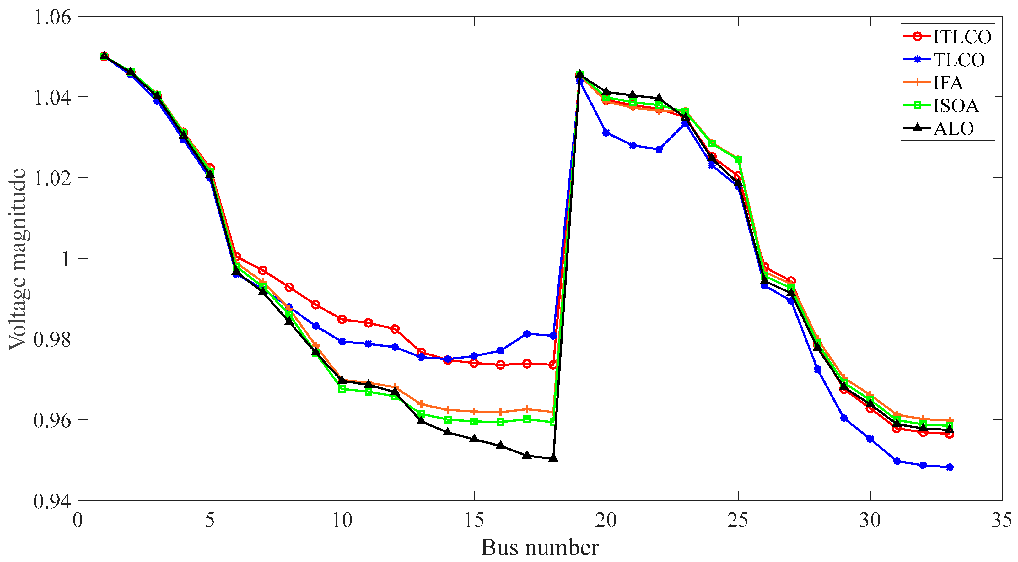
• Thirdly, simulation experiments demonstrate that compared to traditional metaheuristic algorithms such as the ALO, IFA, and IISOA, the proposed method reduces the voltage deviation in the improved IEEE 33-bus system by 4.09% to 14.59%, decreases network losses by 6.65% to 37.52%, and shortens the computation time to 1.49 s.
• Finally, the reconfiguration scheme considering novel load resources can increase the voltage at distant buses by 7.5% and achieve the collaborative optimization of peak–valley difference and network losses, providing theoretical support for the planning and operation of UDNs incorporating VPPs.

Future research can further explore multi-time scale optimization frameworks, collaborative scheduling mechanisms for heterogeneous loads, and the engineering adaptability of the algorithm in larger-scale actual distribution networks.

References

1. Li, H.; Liu, D.; Yao, D.Y. Analysis of the Development of China’s Power System towards Carbon Peak and Carbon Neutrality Goals. Proc. CSEE 2021, 41, 6245–6258. [Google Scholar]
2. Wang, K.; Wang, C.; Yao, W.; Zhang, Z.; Liu, C.; Dong, X.; Yang, M.; Wang, Y. Embedding P2P transaction into demand response exchange: A cooperative demand response management framework for IES. Appl. Energy 2024, 367, 123319. [Google Scholar] [CrossRef]
3. Yu, Y.; Ding, L.; Jin, Z.Y. Robust State Estimation for Active Distribution Networks with Small Sample Imbalance Considering Prediction Assistance. High Volt. Eng. 2024, 50, 4550–4560. [Google Scholar]
4. Zhang, Z.; Hui, H.; Song, Y. Response Capacity Allocation of Air Conditioners for Peak-Valley Regulation Considering Interaction with Surrounding Microclimate. IEEE Trans. Smart Grid 2024, 16, 1155–1167. [Google Scholar] [CrossRef]
5. Zou, Y.; Wang, Q.; Chi, Y.; Wang, J.; Lei, C.; Zhou, N.; Xia, Q. Electric Load Profile of 5G Base Station in Distribution Systems Based on Data Flow Analysis. IEEE Trans. Smart Grid 2022, 13, 2452–2466. [Google Scholar] [CrossRef]
6. Chen, M.; Gao, C.; Shahidehpour, M.; Li, Z.; Chen, S.; Li, D. Internet Data Center Load Modeling for Demand Response Considering the Coupling of Multiple Regulation Methods. IEEE Trans. Smart Grid 2021, 12, 2060–2076. [Google Scholar] [CrossRef]
7. Zhang, M.; Xu, Y.; Sun, H. Optimal Coordinated Operation for a Distribution Network with Virtual Power Plants Considering Load Shaping. IEEE Trans. Sustain. Energy 2023, 14, 550–562. [Google Scholar] [CrossRef]
8. Jia, Z.; Li, J.; Zhang, X.P.; Zhang, R. Review on Optimization of Forecasting and Coordination Strategies for Electric Vehicle Charging. J. Mod. Power Syst. Clean. Energy 2023, 11, 389–400. [Google Scholar] [CrossRef]
9. Mahdavi, M.; Schmitt, K.; Chamana, M.; Bayne, S. Distribution Systems Reconfiguration Considering Dependency of Loads on Grid Voltage and Temperature. IEEE Trans. Power Deliv. 2024, 39, 882–897. [Google Scholar] [CrossRef]
10. Cebeci, C.; Parker, M.; Recalde-Camacho, L.; Campos-Gaona, D.; Anaya-Lara, O. Variable-Speed Hydropower Control and Ancillary Services: A Remedy for Enhancing Grid Stability and Flexibility. Energies 2025, 18, 642. [Google Scholar] [CrossRef]
11. Yu, Y.; Guo, J.; Jin, Z. Optimal Extreme Random Forest Ensemble for Active Distribution Network Forecasting-Aided State Estimation Based on Maximum Average Energy Concentration VMD State Decomposition. Energies 2023, 16, 5659. [Google Scholar] [CrossRef]
12. Tang, J.; Gao, H.C.; Yu, T.; Kang, C. Construction Concept and Innovative Practice of Virtual Power Plants in Megacities under the Electricity Market Environment. Power Syst. Technol. 2025, 49, 103–112. [Google Scholar] [CrossRef]
13. Sun, K.; Liu, J.; Qin, C.; Chen, X. A Method for Optimal Allocation of Distribution Network Resources Considering Power-Communication Network Coupling. Energies 2025, 18, 644. [Google Scholar] [CrossRef]
14. Liu, G.; Cheng, R.; Liu, W.; Shi, Q.; Wang, Z. Enhancing Resilience of Urban Electric-Road-Metro Interdependent Network Considering Electric Bus Scheduling. IEEE Trans. Sustain. Energy 2025, 16, 654–672. [Google Scholar] [CrossRef]
15. Aghdam, F.H.; Javadi, M.S.; Catalão, J.P.S. Optimal Stochastic Operation of Technical Virtual Power Plants in Reconfigurable Distribution Networks Considering Contingencies. Int. J. Electr. Power Energy Syst. 2023, 147, 108799. [Google Scholar] [CrossRef]
16. Wang, L.; Wu, W.; Lu, Q.; Yang, Y. Optimal Aggregation Approach for Virtual Power Plant Considering Network Reconfiguration. J. Mod. Power Syst. Clean. Energy 2021, 9, 495–501. [Google Scholar] [CrossRef]
17. Wang, J.; Pan, Z.; Li, S.; Ge, H.; Yang, G.; Wang, B. Optimal Scheduling of Virtual Power Plant Considering Reconfiguration of District Heating Network. Electronics 2023, 12, 3409. [Google Scholar] [CrossRef]
18. Qiao, X.; Luo, Y.; Xiao, J.; Li, Y.; Jiang, L.; Shao, X.; Cao, Y. Optimal Scheduling of Distribution Network Incorporating Topology Reconfiguration, BES and Load Response: A MILP Model. Chin. Soc. Electr. Eng. J. Power Energy Syst. 2022, 8, 743–756. [Google Scholar]
19. Naderi, E.; Asrari, A. Mitigating Voltage Violations in Smart City Microgrids Under Coordinated False Data Injection Cyberattacks: Simulation and Experimental Insights. Smart Cities 2025, 8, 20. [Google Scholar] [CrossRef]
20. Kanchana, K.; Murali Krishna, T.; Yuvaraj, T.; Sudhakar Babu, T. Enhancing Smart Microgrid Resilience Under Natural Disaster Conditions: Virtual Power Plant Allocation Using the Jellyfish Search Algorithm. Sustainability 2025, 17, 1043. [Google Scholar] [CrossRef]
21. Soesanti, I.; Syahputra, R. Multiobjective Ant Lion Optimization for Performance Improvement of Modern Distribution Network. IEEE Access 2022, 10, 12753–12773. [Google Scholar] [CrossRef]
22. Liu, C. Energy Consumption Prediction and Optimization of Electric Vehicles Based on RLS and Improved SOA. IEEE Access 2024, 12, 38180–38191. [Google Scholar] [CrossRef]
23. Raza, A.; Zahid, M.; Chen, J.; Qaisar, S.M.; Ilahi, T.; Waqar, A.; Alzahrani, A. A Novel Integration Technique for Optimal Location & Sizing of DG Units with Reconfiguration in Radial Distribution Networks Considering Reliability. IEEE Access 2023, 11, 123610–123624. [Google Scholar]
24. Ingalalli, A.; Kamalasadan, S.; Dong, Z.; Bharati, G.R.; Chakraborty, S. Event-Driven Q-Routing-Based Dynamic Optimal Reconfiguration of the Connected Microgrids in the Power Distribution System. IEEE Trans. Ind. Appl. 2024, 60, 1849–1859. [Google Scholar] [CrossRef]
25. Bahrami, S.; Chen, Y.C.; Wong, V.W.S. Dynamic Distribution Network Reconfiguration with Generation and Load Uncertainty. IEEE Trans. Smart Grid 2024, 15, 5472–5484. [Google Scholar] [CrossRef]
26. Zhang, C.; Shan, Y.; Lian, J.; Zhang, C.; Li, M. Optimizing Hydrogen Production for Sustainable Fuel Cell Electric Vehicles: Grid Impacts in the WECC Region. Sustainability 2025, 17, 1129. [Google Scholar] [CrossRef]
27. Atitebi, O.S.; Dumre, K.; Jones, E.C., Jr. Supporting a Lithium Circular Economy via Reverse Logistics: Improving the Preprocessing Stage of the Lithium-Ion Battery Recycling Supply Chain. Energies 2025, 18, 651. [Google Scholar] [CrossRef]
28. Hoang-Le Minh, T.S.; Theraulaz, G.; Abdel Wahab, M.; Cuong-Le, T. Termite Life Cycle Optimizer. Expert Syst. Appl. 2023, 213, 119211. [Google Scholar] [CrossRef]
29. Tong, H.; Zeng, X.; Yu, K.; Zhou, Z. A Fault Identification Method for Animal Electric Shocks Considering Unstable Contact Situations in Low-Voltage Distribution Grids. IEEE Trans. Ind. Inform. 2025, 99, 1–12. [Google Scholar] [CrossRef]
30. Xia, Y.; Li, Z.; Xi, Y.; Wu, G.; Peng, W.; Mu, L. Accurate Fault Location Method for Multiple Faults in Transmission Networks Using Travelling Waves. IEEE Trans. Ind. Inform. 2024, 20, 8717–8728. [Google Scholar] [CrossRef]
Figure 1. The UDN architecture with VPP.
Algorithms 18 00251 g001
Figure 2. Flowchart of the ITLCO algorithm for solving the UDNs incorporating VPPs reconfiguration model.
Algorithms 18 00251 g002
Figure 3. An improved IEEE 33-bus system.
Algorithms 18 00251 g003
Figure 4. The results of the UDN incorporating VPP reconfiguration achieved by the five algorithms.
Algorithms 18 00251 g004
Figure 5. The voltage distribution at each bus of the UDN incorporating VPP after reconfiguration using different algorithms.
Algorithms 18 00251 g005
Figure 6. The energy storage power of buses 16 and 28 changes.
Algorithms 18 00251 g006
Figure 7. Comparison before and after power adjustment of key buses.
Algorithms 18 00251 g007
Figure 8. Voltage distribution at each bus of the UDN incorporating VPP after reconfiguration under different scenarios.
Algorithms 18 00251 g008
Figure 9. The total load variation of UDN within one day.
Algorithms 18 00251 g009