Abstract
Financial time series display inherent nonlinearity and high volatility, creating substantial challenges for accurate forecasting. Advancements in artificial intelligence have positioned deep learning as a critical tool for financial time series forecasting. However, conventional deep learning models often fail to accurately predict future trends in complex financial data due to inherent limitations. To address these challenges, this study introduces a WOA-BiLSTM-ARIMA hybrid forecasting model leveraging parameter optimization. Specifically, the whale optimization algorithm (WOA) optimizes hyperparameters for the Bidirectional Long Short-Term Memory (BiLSTM) network, overcoming parameter tuning challenges in conventional approaches. Due to its strong capacity for nonlinear feature extraction, BiLSTM excels at modeling nonlinear patterns in financial time series. To mitigate the shortcomings of BiLSTM in capturing linear patterns, the Autoregressive Integrated Moving Average (ARIMA) methodology is integrated. By exploiting ARIMA’s strengths in modeling linear features, the model refines BiLSTM’s prediction residuals, achieving more accurate and comprehensive financial time series forecasting. To validate the model’s effectiveness, this paper applies it to the prediction experiment of future spread data. Compared to classical models, WOA-BiLSTM-ARIMA achieves significant improvements across multiple evaluation metrics. The mean squared error (MSE) is reduced by an average of 30.5%, the mean absolute error (MAE) by 20.8%, and the mean absolute percentage error (MAPE) by 29.7%.
1. Introduction
Time series forecasting, a key focus in time series analysis, has been widely applied in fields such as financial markets, transportation, and environmental science [1]. Financial time series holds a central role within the vast and complex landscape of financial big data. Accurately predicting future trends in financial time series is critical for reducing investment risks and ensuring stable financial market operations [2]. However, the high nonlinearity, non-stationarity, and multi-scale volatility of financial markets pose significant challenges to forecasting efforts [3].
Four primary classes of financial time series prediction techniques exist: statistical, machine learning, deep learning, and combined model strategies. Statistical methods, among the earliest widely used for financial time series forecasting, are grounded in robust theoretical foundations. Their core principle involves analyzing historical time series features to construct statistical models for predicting future trends [4]. These methods include established techniques like the Autoregressive Integrated Moving Average (ARIMA) [5] and Generalized Autoregressive Conditional Heteroskedasticity (GARCH) [6] methodologies. Virtanen et al. [7] compared the ARIMA model with multivariate econometric models to forecast the Finnish stock market. Experimental results showed that ARIMA outperformed multivariate econometric models, demonstrating its value in financial market forecasting. Alkamali’s study [8] proposed a time series analysis approach using the ARIMA model for short-term Bitcoin price forecasting. By analyzing Bitcoin price data from 2014 to 2023, the study highlighted ARIMA’s effectiveness in capturing autocorrelation, seasonality, and trends. Li [9] employed past performance data from the Wind financial database, focusing on the SSE 50 ETF and related options, to develop a risk mitigation strategy utilizing GARCH for these options.
In the significant data era, the rapid advancement of computational power and data storage technologies has driven the need for more adaptive algorithms to address the complexity and scale of financial market data [10]. This demand requires surpassing the limitations of traditional time series models and accelerating advancements in machine learning and deep learning within the financial sector. Kim [11] applied Support Vector Machines (SVMs) to predict stock price indices, comparing them with backpropagation neural networks (BP) and case-based reasoning (CBR) to validate SVM’s feasibility in financial forecasting. Zhang et al. [12] proposed a k-fold random forest algorithm based on k-fold cross-validation, named KRF. KRF employs time series analysis models for short-term forecasting of historical data and uses an enhanced random forest algorithm to analyze predictions, enabling dynamic financial crisis warnings. In the evolution of neural networks, Hochreiter et al. [13] initially presented the Long Short-Term Memory (LSTM) architecture. Since its introduction, LSTM has been increasingly applied to financial time series forecasting. To achieve long- and short-term forecasting of horticultural product prices, Banerjee et al. [14] developed an LSTM-based method. This method incorporates historical price data alongside multidimensional factors such as rainfall, exchange rates, and market supply, achieving accurate price predictions via a multivariate LSTM model. Sako et al. [15] explored the use of Recurrent Neural Networks (RNNs) and related models for analyzing financial time series data. These advanced neural network models were used to predict closing prices for eight stock market indices and six USD-related currency exchange rates. Experiments demonstrated that Gated Recurrent Units (GRUs) outperformed others in both univariate and multivariate out-of-sample forecasting.
In time series forecasting, hybrid models have garnered significant attention for their ability to integrate the strengths of different models. Traditional statistical models excel at capturing linear data features, whereas machine learning and deep learning models are adept at modeling nonlinear relationships [16]. Hybrid models address the limitations of single models in handling complex data structures by separately modeling linear and nonlinear components. Zhang et al. [17] combined Complementary Ensemble Empirical Mode Decomposition (CEEMD), Principal Component Analysis (PCA), and LSTM to develop the CEEMD-PCA-LSTM model. Empirical studies on six representative stock indices across three distinct markets validated the model’s accuracy in stock market forecasting. He et al. [18] combined deep learning techniques with conventional time series analysis to develop an innovative hybrid forecasting framework called ARMA-CNN-LSTM. This cutting-edge model effectively identifies and processes both linear patterns and complex nonlinear relationships within financial market data, offering superior predictive performance compared to standalone approaches. Song et al. [19] used Variational Mode Decomposition (VMD) to extract predictive features from shipping market time series data, followed by forecasting with Light Gradient Boosting Machine (LightGBM). Liu et al. [20] integrated the Flexible Dendritic Neuron Model (FDNM) and Dendritic Gated Recurrent Network (DGRNet) to propose an advanced forecasting framework, FD-GRNet. FDNM’s dendritic mechanism substantially improves the model’s capture of intricate nonlinearities. Meanwhile, DGRNet enhances the model’s capacity to handle temporal dependencies. By leveraging these strengths, FD-GRNet effectively manages long-term dependencies and nonlinear patterns in financial market data.
However, existing hybrid forecasting models still have several limitations, such as issues with hyperparameter optimization. To address hyperparameter optimization, researchers have proposed various hybrid algorithms combining metaheuristic methods with deep learning models. Singh et al. [21] utilized a genetic algorithm (GA) to optimize LSTM parameters, demonstrating the effectiveness of parameter optimization through comparative testing on the National Stock Exchange-Fifty dataset. Tang et al. [22] employed a particle swarm optimization (PSO) algorithm to optimize GRU parameters, proposing a model for predicting Bitcoin volatility that supports risk warning and butterfly option arbitrage strategies. Although these hybrid models address parameter optimization, they do not consider the performance of the optimization algorithms themselves, such as computational complexity or the balance between global search and local exploitation capabilities. On the other hand, most existing methods lack adequate handling of data nonlinearity and post-processing mechanisms for prediction errors, making it difficult to dynamically correct prediction biases.
To address the limitations of prior approaches, we propose a novel hybrid forecasting model, WOA-BiLSTM-ARIMA, integrating the whale optimization algorithm [23], bidirectional long short-term memory networks, and the autoregressive integrated moving average model. In the proposed model, WOA offers greater portability compared to other metaheuristic algorithms while balancing strong global search and local exploitation capabilities, enabling the identification of optimal BiLSTM hyperparameter combinations with fewer computational resources, thus effectively addressing parameter selection challenges and enhancing predictive performance. The model leverages BiLSTM’s capability to fit nonlinear data and ARIMA’s strength in processing linear data, capturing complex features while maintaining the stability of traditional statistical models, thereby significantly improving forecasting accuracy.
2. Data Description
2.1. Data Source
This research examines price differentials between rebar (RB) and hot-rolled coil (HC) futures contracts on the Shanghai Futures Exchange, spanning 30 September 2014 to 30 September 2024. The price data for both steel products were derived from high-frequency trading data recorded every 5 min, from which the price differences were calculated to form a price spread data series. The dataset comprises a total of 18,000 data points. Table 1 presents various indicators of the data characteristics.

Table 1.
Data characterization selection indicators.
2.2. Cointegration Tests
Prior to arbitrage trading, paired commodity contracts should exhibit a long-term stable cointegration relationship [24]. Cointegration implies that, despite individual price fluctuations, a predictable long-term equilibrium relationship exists between the two commodities. This study aims to explore price spread arbitrage opportunities between RB and HC, making it essential to verify the presence of a cointegration relationship between their prices.
Figure 1’s RB and HC closing price trends indicate a possible relationship. To quantitatively assess this relationship, we conducted Augmented Dickey–Fuller (ADF) stationarity tests [25] on the closing price series of rebar and hot-rolled coil to determine if both are integrated of the same order. Table 2 summarizes the ADF test results for the closing price series. The p-values of the original series exceed 0.05, indicating that both are non-stationary in their raw form. After first-order differencing, the p-values fall below 0.05, and the ADF statistics are below the critical value, confirming that the differenced series are stationary and both are integrated of order one.
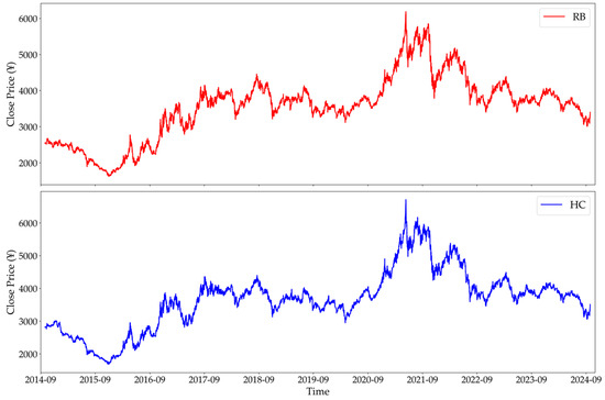
Figure 1.
Timing charts of closing prices for RB and HC.
Table 2.
ADF test results for the closing prices of RB and HC.
Having confirmed that the original price series of RB and HC are non-stationary but become stationary after first-order differencing, we proceeded with the Engle–Granger cointegration test [26]. The first step involves constructing a long-term equilibrium relationship model, with its mathematical expression presented in Equation (1),
where and denote the closing prices of HC and RB, respectively, represents the cointegration coefficient, and denotes the residual.
The second step involves conducting an ADF test on the residual term to assess its stationarity. Table 3 presents the ADF test results for the residuals. The Augmented Dickey–Fuller test results show that the residual series is a stationary sequence, with the ADF statistic falling well below the critical threshold and a statistically significant p-value under 0.05. This provides strong evidence of cointegration between RB and HC prices, validating the potential for implementing a pairs trading strategy between these commodities.
Table 3.
ADF test results for residual values.
We tested the price spread series for stationarity to assess the model’s data-fitting performance. According to the ADF test results for the price spread series between RB and HC shown in Table 4, the p-value is less than 0.05, and the ADF statistic is below the critical value, indicating that the fitted price spread series is stationary. Thus, the rationality and effectiveness of subsequent modeling are validated.
Table 4.
ADF test results for the spread series.
3. Methods
3.1. ARIMA
The ARIMA model, a statistical method for analyzing and predicting time series data, combines autoregressive (AR), integrated (I), and moving average (MA) elements [5]. The AR element delineates the correlation between a time series and its preceding data points. The I element addresses non-stationary series by employing differencing for conversion into a stationary form. The MA element simulates the relationship linking present values to prior prediction inaccuracies. ARIMA leverages these three components to convert non-stationary series into stationary ones for modeling. Given a time series , the ARIMA modeling process can be described by the following steps.
The parameter (d) in the ARIMA (p, d, q) model represents the number of differences required to transform a non-stationary series into a stationary one. If a single difference () is insufficient to achieve stationarity, multiple differences may be applied. The stationary series after differencing can be modeled by an ARMA (p, q) model, as expressed in Equation (2),
where represents the autoregressive coefficients, denotes the moving average coefficients, and is the random error term.
The order of the ARIMA model is defined by the autoregressive order , differencing order , and moving average order q, which are determined through a grid search to find the optimal (p, d, q) combination. To evaluate model performance, the Akaike Information Criterion (AIC) was used as the evaluation metric. For each candidate parameter combination (p, d, q) in the grid search, maximum likelihood estimation (MLE) was used to fit the model, and the corresponding AIC value was calculated. The parameter combination with the smallest AIC value was ultimately selected as the optimal model. This exhaustive search method ensured the fairness of comparisons by re-estimating model parameters for each parameter configuration. The calculation of AIC is given by Equation (3). During parameter selection, the grid search spans the autoregressive order , differencing order , and moving average order . This process identifies the optimal (p, d, q) combination for the ARIMA model.
where represents the likelihood function value, is the log-likelihood, and is the number of model parameters.
After determining the model order, MLE was used to estimate the parameters of the ARMA model, including the autoregressive coefficients, moving average coefficients, and error variance . During the estimation process, it was assumed that the error term is mutually independent and identically distributed, following a normal distribution with zero mean and constant variance. Under this assumption, the resulting likelihood function is the Gaussian pseudo-likelihood, as shown in Equation (4),
where is the parameter vector to be estimated, and is the error term.
This assumption enables the calculation of the log-likelihood function used for AIC evaluation, as shown in Equation (5),
3.2. BiLTM
In 1997, Hochreiter et al. first proposed the LSTM structure, introducing input, forget, and output gate mechanisms, effectively mitigating the gradient vanishing and exploding problems prevalent in RNNs during long-sequence learning [27]. The LSTM structure excels in time series modeling, capable of capturing long-term dependencies, and is an important tool for handling sequence prediction tasks.
However, traditional LSTM networks have limitations in certain tasks, particularly in scenarios requiring simultaneous consideration of historical information and future context. To address this issue, researchers proposed BiLSTM network structure [28]. BiLSTM simultaneously uses two LSTM layers: one processes the sequence forward in time to capture dynamic features from the past to the present, while the other processes the sequence backward in time to extract dependency information from the future to the present. This bidirectional information flow structure enables BiLSTM to comprehensively capture contextual information at each time step, thereby outperforming unidirectional LSTM in modeling complex temporal features. Figure 2 illustrates the structure of the BiLSTM model.
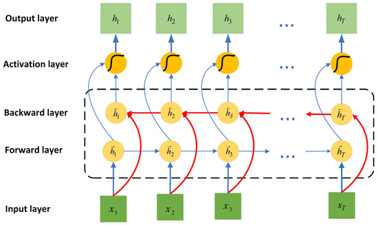
Figure 2.
Architecture of the BiLSTM model.
For an input sequence , the forward LSTM layer’s output at time step is computed using Equations (6)–(11),
where denotes the forward LSTM output from the preceding time interval, denotes the input gate’s activation, controlling how much of input is written to the cell state, represents the concatenation operation between two feature vectors, is the forget gate’s activation, determining the proportion of retained cell state information, and represent the candidate and updated cell states, respectively, is the output gate’s activation, regulating the output information from the cell state, , , , and denote weight matrices, , , , and are corresponding bias terms, and is the sigmoid activation function, introducing nonlinear transformations.
The backward LSTM layer obtains its output according to the same computational procedure. Ultimately, the outputs of the forward and backward LSTM layers are concatenated along the feature dimension to obtain the output of the entire BiLSTM network. At time step t, the information fusion process is as shown in Equation (12),
where and represent the forward LSTM layer and the backward LSTM layer, respectively.
3.3. WOA
The whale optimization algorithm is a nature-inspired heuristic optimization algorithm based on swarm intelligence, drawing inspiration from the bubble-net feeding behavior of humpback whales during predation. This algorithm achieves effective solutions to complex optimization problems by simulating the prey-capturing strategies of whales. The main processes of WOA include three stages: encircling prey, bubble-net attacking, and searching for prey. The specific pseudocode, as shown in Algorithm 1, provides a detailed description of the algorithm’s implementation process.
| Algorithm 1. Whale optimization algorithm (WOA) |
| Input: Objective function , population size , maximum iterations Max Output: Best solution and its fitness |
| 1: Initialize the whale population 2: Evaluate the fitness of each whale f(x) 3: Identify the best solution 4: For to do: 5: For each whale = 1 to : 6: Calculate parameter 7: Generate random numbers and in [0, 1] 8: Compute 9: Compute 10: Generate in [0, 1] 11: If then 12: If then 13: Compute 14: Update 15: Else 16: Choose randomly from the population 17: Compute 18: Update 19: Else 20: Compute 21: Generate in [−1, 1] 22: Set (a constant, typically = 1) 23: Update 24: Update fitness of all whales 25: Update if a better solution is found 26: Return and |
Assume a D-dimensional search space, with whale position , where and stands for population size. During prey encirclement, whales assume the best individual’s position as the target, guiding others to reposition. The distance vector between a whale’s current position and the optimal individual is calculated per Equation (13), with its new position in the next iteration given by Equation (14),
where denotes the global optimal position at iteration , and represents the whale’s current position. Coefficient vectors and , controlling perturbation and search ranges, are defined by Equations (15) and (16),
where linearly decreases from 2 to 0, balancing local and global search, and and are random vectors between 0 and 1.
In the bubble-net attack phase, a spiral equation between whale and prey simulates humpback whale rotation, computed via Equations (17) and (18),
where is a constant controlling the spiral shape, and is a random value in the range [−1, 1].
The choice between encircling prey and a spiral attack is made randomly. Assuming a 50% probability for each behavior, encircling prey is selected when probability applies, otherwise spiral attack, as expressed in Equation (19),
During the search-for-prey phase, when the condition holds, other whales update their positions based on a randomly selected whale’s position. This mechanism enhances the algorithm’s exploration capability, enabling WOA to perform a global search. This process is described by Equations (20) and (21),
where denotes the position of a randomly selected whale from the current population.
Figure 3 shows the implementation process of the WOA.
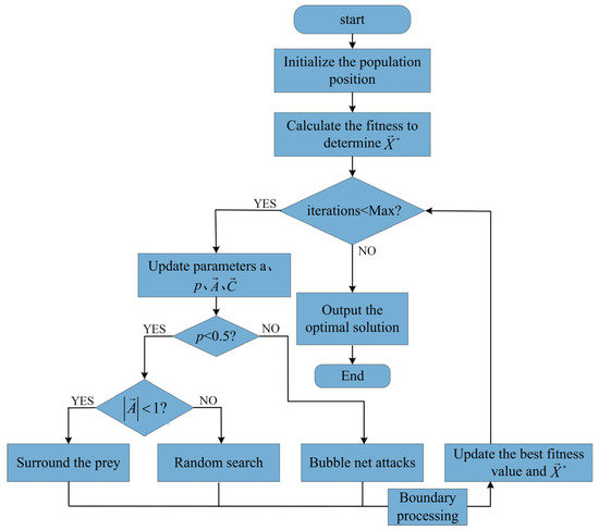
Figure 3.
Flowchart of the WOA.
3.4. WOA-BiLSTM-ARIMA Hybrid Model
The proposed WOA-BiLSTM-ARIMA hybrid model effectively integrates ARIMA’s linear feature modeling with BiLSTM’s nonlinear feature capture. Additionally, incorporating the WOA optimizes model parameters, leveraging its global search efficiency to enhance forecasting performance. Figure 4 illustrates the WOA-BiLSTM-ARIMA framework.
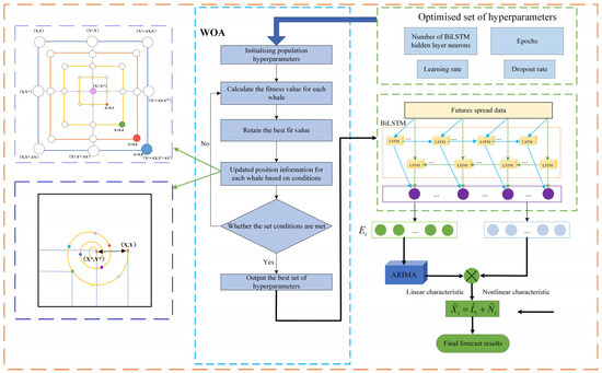
Figure 4.
Architecture of the WOA-BiLSTM-ARIMA model.
The price spread series of rebar and hot-rolled coil steel products serves as the model’s input. Initially, is preprocessed and segmented into multidimensional training samples using a sliding window mechanism [29]. Subsequently, the WOA conducts iterative searches to determine the optimal hyperparameter combination for the BiLSTM model. After parameter optimization, the configured BiLSTM network models nonlinear features, outputting nonlinear predictions and residuals . The residual series is input to the ARIMA model to capture linear features . Finally, a feature fusion layer integrates BiLSTM’s nonlinear predictions with ARIMA’s linear features to produce the final forecast .
The complete dataset comprises two types of data: nonlinear data and linear data . The data to be predicted, , can be expressed by Equation (22),
The WOA-BiLSTM model predicts the nonlinear component of , yielding the predicted nonlinear values , as described by Equations (23) and (24),
where denotes the nonlinear transformation, and are the weight matrices for the forward LSTM, and for the backward LSTM, and are the respective forward and backward bias terms, is the weight matrix of the output layer, is its corresponding bias term, and is the nonlinear activation function. The nonlinear transformation overcomes the model’s linear constraints, significantly enhancing BiLSTM’s ability to represent high-noise sequential data.
After obtaining the nonlinear features for both the training and test sets, the residual values of the WOA-BiLSTM model on the training set can be derived using the training set data and the predicted nonlinear data , as expressed by Equation (25),
Subsequently, the residual sequence from the training set is used as input to the ARIMA model to predict the linear component , which the WOA-BiLSTM model struggles to accurately predict on the test set. The prediction of the linear features is given by Equation (26),
where and represent the autoregressive order and moving average order, respectively, represents the residual values on the training data, and correspond to the autoregressive and moving average terms, respectively, and represents the white noise term.
To achieve effective prediction of the BiLSTM training residual data, the ARIMA model in this paper adopts a rolling prediction approach. Specifically, after each prediction, the new predicted value is added to the training data, and the ARIMA model is refitted to update the parameters , , and . Parameter updates are based on the grid search functionality of the pmdarima library, which searches for the optimal parameter combination within a predefined range to dynamically respond to structural changes in the time series. This dynamic adjustment mechanism enhances the model’s adaptability to data drift and non-stationarity, thereby improving prediction accuracy. The specific process of rolling prediction is illustrated in Figure 5.
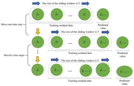
Figure 5.
Rolling forecast of the ARIMA model.
Let the input residual data be . Initialize the training set and set the sliding window length to , with here denoting the length of the entire training set, and with a prediction step size of 1. After each prediction, the predicted residual for the next time step is added to the training data, while the residual from the first time point is removed to maintain a window length of . Subsequently, the ARIMA model is re-estimated. Through this rolling prediction approach, the ARIMA model effectively captures local trends and short-term fluctuations, thereby enhancing short-term prediction performance.
Finally, the nonlinear features from the WOA-BiLSTM model on the test set are combined with the linear features predicted by the ARIMA model to obtain the final prediction results on the test set, as expressed by Equation (27),
3.5. Evaluation Metrics
In order to meticulously measure the predictive prowess in various experimental conditions, the research utilizes the mean squared error, mean absolute error, and mean absolute percentage error metrics to gauge the precision of the forecasts. MSE measures the average squared difference between predicted and actual values. MAE reflects the average absolute difference between predicted and actual values. MAPE provides the average percentage error relative to the actual values. Typically, smaller metric values reflect enhanced model effectiveness, with specific calculations detailed in Equations (28)–(30),
where represents the actual value, the predicted value, and represents the number of samples in the test set.
4. Experiment
4.1. Experimental Settings
In our experiments, the WOA-BiLSTM-ARIMA model was implemented using Python 3.7 and TensorFlow 2.5, and executed on a hardware environment equipped with an Intel(R) Xeon(R) W-2225 CPU @ 4.10 GHz (Intel Corporation, Santa Clara, CA, USA) and an NVIDIA RTX A6000 (NVIDIA Corporation, Santa Clara, CA, USA). Here, WOA was implemented based on Numpy 1.21.6, BiLSTM was constructed using the TensorFlow 2.5.0 framework, and the ARIMA model was built by invoking Statsmodels 0.13.2. Table 5 provides detailed information on the hardware and key software packages used in the experiments.
Table 5.
Experimental environment configuration.
We analyzed the average runtime of the complete prediction pipeline to provide a reference for computational efficiency. In a server environment equipped with an NVIDIA RTX A6000 GPU and an Intel(R) Xeon(R) W-2225 CPU @ 4.10 GHz, with a batch size of 4096, the entire prediction process took approximately 149,168 s. Of this, the WOA-BiLSTM model’s training and prediction processes accounted for approximately 57.9% of the total time, while the ARIMA module’s nonlinear prediction and residual correction processes contributed about 42.1%.
4.2. Data Processing
In this study, the futures spread dataset used includes eight indicators, including the closing price. To meet the input requirements of the WOA-BiLSTM component in the WOA-BiLSTM-ARIMA model, the data must be preprocessed to conform to a multi-feature input and single-feature output format. Specifically, the data needs to be divided into multi-step training data and their corresponding target values, i.e., using multiple historical data points to predict a single target value. The data division method is illustrated in Figure 6. Assuming the dataset contains historical records, the time step is set to S, and the target value is the closing price spread at time . Using a sliding window of size 15, the data was incrementally transformed into a multi-step, multi-feature format to meet the training requirements of the WOA-BiLSTM model. For the ARIMA model, the input data consists of the single-feature closing price spread residual data output by the WOA-BiLSTM model on the training set.
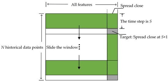
Figure 6.
Input data processing.
After data division, 60% of the data is used as the training set, 20% as the validation set, and the remaining 20% as the test set. To improve training efficiency and accelerate convergence, the data is normalized before use, scaling each feature value to the [0, 1] interval. Equation (31) describes the normalization process,
where represents the data at the -th time point, while and denote the minimum and maximum values of the entire dataset, respectively.
4.3. Optimizing Network Parameters by the WOA
To find the optimal hyperparameter combination, WOA is employed to optimize the hyperparameters of the BiLSTM model. The objective of WOA is to optimize model performance by minimizing the mean squared error on the validation set. The optimized hyperparameters include the count of neurons in the BiLSTM’s concealed layers, the learning pace, the dropout proportion, and the epoch limit for training.
To avoid blind hyperparameter searches and improve efficiency, the search ranges for each hyperparameter are constrained based on related studies [30,31], with specific ranges listed in Table 6. During optimization, both the number of whales and iterations are set to 10. After 10 iterations, the optimal hyperparameters are as follows: the number of neurons in the three hidden layers is 462, 214, and 270, respectively; the learning rate is 0.0004; the dropout rates are 0.7712 and 0.3356; and the number of training epochs is 428. These results are also recorded in Table 6.
Table 6.
Hyperparameter optimization results.
Figure 7 visually illustrates the dynamic changes in hyperparameters and the fitness function under the influence of the WOA. In the early stages of optimization, the fitness value shows a rapid decline, indicating a swift improvement in model performance. After seven iterations, the fitness value stabilizes, and the hyperparameters cease to change, indicating that the algorithm has successfully identified the optimal hyperparameter combination.
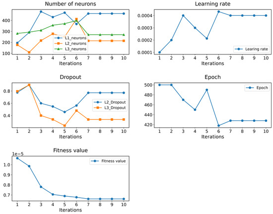
Figure 7.
The process of hyperparameter variation.
Figure 8 illustrates the loss trends of the BiLSTM model during training and validation. As shown in Figure 8, both training and validation losses consistently decreased with increasing iterations, converging to similar low values in later stages. The absence of significant divergence between the two loss curves indicates stable model performance on the validation set, with no evident signs of overfitting. Furthermore, Figure 8 shows that training terminated before reaching the preset maximum number of epochs, owing to the implementation of an early stopping strategy. In the early stopping strategy, we set the monitor to val_loss, patience to 20, min_delta to 0.00001, and enabled restore_best_weights. Specifically, early stopping is triggered when the validation loss fluctuation remains below 0.00001 for 20 consecutive epochs, and the model saves and restores the best weights to effectively reduce the risk of overfitting due to prolonged training. Additionally, during training, we applied Dropout regularization, randomly deactivating certain neurons to encourage the model to learn more generalizable features, further alleviating overfitting. During validation, all neurons were activated, enabling the model to leverage diverse feature representations for stable predictive performance. These measures collectively enhanced the model’s generalization ability beyond the training data.
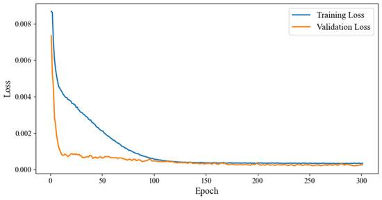
Figure 8.
Comparison between training loss and validation loss.
4.4. Results and Analysis
To evaluate the proposed model’s performance, we conducted comparative experiments with common financial time series forecasting models, including BP neural networks, RNN, LSTM, GRU, and Transformer. All models adopt the same prediction approach as WOA-BiLSTM-ARIMA, using multi-step, multi-feature inputs to produce single-step, single-feature outputs. These models encompass the primary techniques for predicting financial time series trends. Figure 9 and Table 7 illustrate findings from testing.
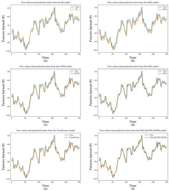
Figure 9.
Comparison between predicted and actual values of models. (a) BP model. (b) RNN model. (c) LSTM model. (d) GRU model. (e) Transformer model. (f) Proposed model.
Table 7.
Forecasting results of different models.
Figure 9 illustrates the comparison between the predicted results of various models and the actual values on the test set. In Figure 9, the vertical axis represents the closing price spread, and the horizontal axis label “Time” denotes the time steps, with each step corresponding to a sampling interval of 5 min. The figure plots the prediction results for the first 300 time steps of the test set. It can be observed from the figure that the proposed WOA-BiLSTM-ARIMA model outperforms other comparative models in terms of the fit between predicted and actual values, with the closest trend alignment. This indicates that the model exhibits superior prediction accuracy and generalization ability in the closing price spread prediction task.
In the quantitative analysis of the experiments, we calculated and analyzed the performance of WOA-BiLSTM-ARIMA compared to other models across various evaluation metrics. In terms of MSE, WOA-BiLSTM-ARIMA improves by 45.6%, 35.6%, 21.3%, 26.6%, and 14.4% compared to BP, RNN, LSTM, GRU, and Transformer, respectively. Additionally, regarding MAE and MAPE metrics, WOA-BiLSTM-ARIMA significantly outperforms all comparative models. It can be concluded that the WOA-BiLSTM-ARIMA consistently achieves better performance than other comparative models.
To investigate the interaction mechanisms among the components of the hybrid model, the WOA-BiLSTM-ARIMA model was sequentially decomposed into ARIMA, BiLSTM, WOA-BiLSTM, and BiLSTM-ARIMA structures for ablation (i.e., component removal) comparison experiments, with results shown in Table 8. The results show that WOA-BiLSTM and WOA-BiLSTM-ARIMA outperform BiLSTM and BiLSTM-ARIMA without WOA in prediction performance, with model performance improving by 4.9% and 8.4% in MSE metrics after incorporating WOA, powerfully demonstrating the effectiveness of WOA in hyperparameter selection. Additionally, the BiLSTM-ARIMA model achieves MSE, MAE, and MAPE values of 6.3493, 1.7544, and 2.5832%, respectively, outperforming standalone BiLSTM and ARIMA models, thus validating the effectiveness of this integrated architecture in improving prediction performance. By comparing the results of decomposed and combined models, the practical value and advantages of the proposed hybrid modeling strategy in financial time series forecasting tasks are further confirmed.
Table 8.
Ablation experiment results.
To further evaluate the unconditional predictive performance of the proposed WOA-BiLSTM-ARIMA model (Base) against comparison models (BP, RNN, LSTM, GRU) and ablation models (BiLSTM, ARIMA, WOA-BiLSTM, BiLSTM-ARIMA), we employed the Giacomini–White (GW) test method [32]. By constructing regression models under a given loss function, we tested whether there were significant differences in the predictive performance of the models. Following the GW test method, we calculated the p-value after constructing the corresponding regression models. A p-value less than 0.05 indicates a significant difference in performance between the two models under the given conditions. A p-value greater than 0.05 suggests no statistically significant difference in predictive performance between the two models. When the significance condition (p < 0.05) is met, the sign of the GW statistic (GWstat) can further determine the relative superiority of the models. A GWstat greater than 0 indicates that the Base model outperforms the comparison model, while the opposite suggests the comparison model is superior. The GW test results, as shown in Table 9, indicate that all p-values are less than 0.05, with positive GWstat values. These results demonstrate that the WOA-BiLSTM-ARIMA model significantly outperforms all baseline and ablation models, exhibiting a clear advantage in predictive performance.
Table 9.
Results of the GW tests.
The superior performance of the WOA-BiLSTM-ARIMA model in experiments can be attributed to its structural integration of linear and nonlinear strengths, complemented by precise parameter calibration via WOA. Specifically, ARIMA effectively captures linear trends in financial time series, while BiLSTM, with its bidirectional recurrent mechanism, models nonlinear dynamics and long-term dependencies within the sequence. The introduction of WOA enhances BiLSTM hyperparameter optimization by providing global search capabilities, effectively mitigating the local optima issues associated with traditional manual tuning. Furthermore, we employed ARIMA for secondary modeling of BiLSTM residuals, enabling compensatory corrections for unmodeled linear structures, thereby significantly reducing overall prediction errors. This hybrid architecture maintains high sensitivity to linear patterns while excelling in capturing complex nonlinear patterns, ultimately enhancing the model’s overall performance in financial time series forecasting tasks.
4.5. Walk-Forward Validation
To evaluate the model’s generalization ability across different periods in a non-stationary financial environment, we introduced the walk-forward validation strategy. This strategy closely aligns with real-world deployment scenarios, where the model is trained solely on historical data and predicts future unknown data, effectively avoiding information leakage. The experiment selected a time range from 30 September 2014 to 1 July 2024, covering multiple market cycles with good structural diversity. The initial training set period was from 30 September 2014 to 1 January 2021. We set the sliding window step size to 6 months. In each validation round, the training set includes all historical data from the start time to the current validation point, followed by evaluating the model’s predictive performance over the next 6 months. After validation, the training set time range is rolled forward by 6 months, the model is retrained, and the next 6-month period is predicted. A total of 5 rounds of walk-forward validation were conducted, with the test period covering January 2022 to July 2024. We reported MSE, MAE, and MAPE metrics for each test phase to measure the model’s predictive stability and generalization ability across different time periods. The experimental results are shown in Table 10.
Table 10.
Walk-forward validation results with cumulative training.
From the results in Table 10, it can be seen that the model’s MSE, MAE, and MAPE remained at low levels across all stages from Fold 1 to Fold 5, with no significant fluctuations. Specifically, MSE steadily decreased from 6.4452 to a minimum of 4.2137, MAE fluctuated between 1.8738 and 1.2694, and MAPE consistently remained between 1% and 7%. This indicates that the proposed model has good temporal stability and strong generalization ability, capable of adapting to long-term structural changes in non-stationary financial markets, demonstrating potential for sustained operation in real-world deployment.
4.6. Backtesting Experiment
This study used 5 min K-line data of hot-rolled coil from 2019 to 2024 for backtesting, with concurrent 5 min K-line data of rebar as training samples, to systematically compare three strategies: R-Breaker, R-Breaker-WOA-BiLSTM (R-Breaker-WB), and R-Breaker-WOA-BiLSTM-ARIMA (R-Breaker-WBA). In the R-Breaker-WB strategy, we first globally optimized BiLSTM hyperparameters using WOA, followed by directional predictions of price movements over the next 5 min. Simultaneously, the six key thresholds of R-Breaker—breakout buy price, observation sell price, reversal sell price, reversal buy price, observation buy price, and breakout sell price—were dynamically adjusted based on prediction results to enable real-time corrections of entry and exit signals. The R-Breaker-WBA strategy further incorporates ARIMA at the residual level to perform secondary modeling and compensation of BiLSTM prediction errors, thereby refining trading signals. All backtesting results are summarized in Table 11.
Table 11.
Comparison of backtesting results.
As shown in Table 11, under the same initial capital conditions, R-Breaker-WBA achieved the highest final equity, with a total return of 105.7% and an annualized return of 21.14%, significantly outperforming R-Breaker-WB and the original R-Breaker. Despite R-Breaker-WBA having the highest trading frequency, its profitable trade ratio reached 59.7%, indicating robust signal quality. Notably, its Sharpe ratio of 0.88 far exceeds that of R-Breaker-WB (0.43) and R-Breaker (−0.74), demonstrating significantly improved risk-adjusted returns despite similar or higher risk exposure. R-Breaker-WB also achieved excess returns compared to the baseline strategy, further validating the effectiveness of integrating deep learning prediction modules with classical trading strategies.
5. Conclusions
This study proposes a hybrid forecasting model, WOA-BiLSTM-ARIMA, integrating the whale optimization algorithm to achieve precise modeling and prediction of financial time series. The model employs WOA to dynamically optimize BiLSTM hyperparameters, effectively mitigating the subjectivity of traditional manual parameter tuning and enhancing prediction accuracy. Structurally, WOA-BiLSTM-ARIMA integrates BiLSTM’s ability to capture complex nonlinear patterns with ARIMA’s strengths in modeling linear trends and residual correction, forming an integrated dual-modeling framework that synergistically optimizes prediction accuracy and robustness. This study addresses the gap in high-performance automated parameter tuning and error-adaptive mechanisms for deep learning models in short-term futures spread arbitrage, providing a new pathway for intelligent financial modeling in high-frequency trading and arbitrage strategies.
Practically, this study uses rebar and hot-rolled coil spread data, constructing a multidimensional input feature system incorporating technical indicators and historical market data, with closing prices as the prediction target, to systematically evaluate the model’s performance in real market environments. The experiments employed multiple error evaluation metrics, including MSE, MAE, and MAPE, and used the Giacomini–White test to verify the statistical significance of prediction accuracy differences, ensuring the reliability and scientific rigor of the results. Compared to various mainstream time series forecasting methods, the WOA-BiLSTM-ARIMA model demonstrates significant advantages in prediction accuracy, particularly for short-term spread arbitrage scenarios. Furthermore, through backtesting analysis based on prediction results, the model was integrated with the R-Breaker trading strategy, validating its profitability and risk control effectiveness in arbitrage strategy execution, providing strong support for its practical application value.
In the increasingly competitive financial market environment, the WOA-BiLSTM-ARIMA model effectively extracts data features and accurately predicts financial data. However, the model still has certain limitations. The WOA may encounter slow convergence or local optima issues in high-dimensional search spaces, impacting optimization effectiveness. The BiLSTM-ARIMA structure exhibits some capability in modeling short-term fluctuations but may show delayed responses under extreme market sentiments or sudden events. The model’s training and prediction processes also incur relatively high computational costs. Future research will optimize the WOA to enhance global search capabilities, employ feature selection techniques to identify key features, and integrate multi-source data to further improve the model’s predictive performance.
Author Contributions
Conceptualization, B.Y.; Methodology, B.Y.; Software, P.Q.; Validation, Z.C.; Formal analysis, Z.G.; Investigation, Y.D.; Writing—original draft, B.Y.; Writing—review and editing, B.Y.; Visualization H.Q.; Supervision, P.Q.; Project administration, P.Q.; Data curation, Y.L. All authors have read and agreed to the published version of the manuscript.
Funding
This work was supported by the National Natural Science Foundation of China (Grant No. 62472144), Henan Province Key R&D and Promotion Special Project (Soft Science) (Grant No.252400410396), and the “Science and Technology Innovation Yongjiang 2035” Major Application Demonstration Plan Project in Ningbo (Grant No. 2024Z005). The funders are responsible for the entire program.
Data Availability Statement
The raw data supporting the conclusions of this article will be made available by the authors upon request.
Conflicts of Interest
The authors declare no conflicts of interest.
References
- Alsharef, A.; Aggarwal, K.; Sonia; Kumar, M.; Mishra, A. Review of ML and AutoML solutions to forecast time-series data. Arch. Comput. Methods Eng. 2022, 29, 5297–5311. [Google Scholar] [CrossRef]
- Yang, Y. Research on financial investment risk assessment techniques and applications. Sci. Technol. Soc. Dev. Proc. Ser. 2024, 2, 117–123. [Google Scholar] [CrossRef]
- Huang, S.; An, H.; Gao, X.; Hao, X.; Huang, X. The multiscale conformation evolution of the financial time series. Math. Probl. Eng. 2015, 2015, 563145. [Google Scholar] [CrossRef]
- Usmani, U.A.; Aziz, I.A.; Jaafar, J.; Watada, J. Deep learning for anomaly detection in time-series data: An analysis of techniques, review of applications, and guidelines for future research. IEEE Access 2024, 12, 174564–174590. [Google Scholar] [CrossRef]
- Box, G.E.P.; Jenkins, G.M.; Reinsel, G.C.; Ljung, G.M. Time Series Analysis: Forecasting and Control, 5th ed.; John Wiley Sons: Hoboken, NJ, USA, 2015. [Google Scholar]
- Bollerslev, T. Generalized autoregressive conditional heteroskedasticity. J. Econom. 1986, 31, 307–327. [Google Scholar] [CrossRef]
- Virtanen, I.; Yli-Olli, P. Forecasting stock market prices in a thin security market. Omega 1987, 15, 145–155. [Google Scholar] [CrossRef]
- Alkamali, A. Bitcoin Short-Term Price Prediction Using Time Series Analysis; Rochester Institute of Technology: Rochester, NY, USA, 2024. [Google Scholar]
- Li, J. Research on risk hedging strategy of SSE 50ETF options based on GARCH model. Econ. Issues 2023, 45, 68–75. [Google Scholar]
- Karanam, R.K.; Natakam, V.M.; Boinapalli, N.R.; Sridharlakshmi, N.R.B.; Allam, A.R.; Gade, P.K.; Manikyala, A. Neural networks in algorithmic trading for financial markets. Asian Account. Audit. Adv. 2018, 9, 115–126. [Google Scholar]
- Kim, K.J. Financial time series forecasting using support vector machines. Neurocomputing 2003, 55, 307–319. [Google Scholar] [CrossRef]
- Zhang, C.; Zhong, H.; Hu, A. Research on early warning of financial crisis of listed companies based on random forest and time series. Mob. Inf. Syst. 2022, 2022, 1573966. [Google Scholar] [CrossRef]
- Hochreiter, S.; Schmidhuber, J. Long short-term memory. Neural Comput. 1997, 9, 1735–1780. [Google Scholar] [CrossRef]
- Banerjee, T.; Sinha, S.; Choudhury, P. Long term and short term forecasting of horticultural produce based on the LSTM network model. Appl. Intell. 2022, 52, 9117–9147. [Google Scholar] [CrossRef]
- Sako, K.; Mpinda, B.N.; Rodrigues, P.C. Neural networks for financial time series forecasting. Entropy 2022, 24, 657. [Google Scholar] [CrossRef]
- Benidis, K.; Rangapuram, S.S.; Flunkert, V.; Wang, Y.; Maddix, D.; Turkmen, C.; Januschowski, T. Deep learning for time series forecasting: Tutorial and literature survey. ACM Comput. Surv. 2022, 55, 1–36. [Google Scholar] [CrossRef]
- Zhang, Y.A.; Yan, B.; Aasma, M. A novel deep learning framework: Prediction and analysis of financial time series using CEEMD and LSTM. Expert Syst. Appl. 2020, 159, 113609. [Google Scholar] [CrossRef]
- He, K.; Yang, Q.; Ji, L.; Pan, J.; Zou, Y. Financial time series forecasting with the deep learning ensemble model. Mathematics 2023, 11, 1054. [Google Scholar] [CrossRef]
- Song, X.; Chen, Z.S. Enhancing financial time series forecasting in the shipping market: A hybrid approach with Light Gradient Boosting Machine. Eng. Appl. Artif. Intell. 2024, 136, 108942. [Google Scholar] [CrossRef]
- Liu, T.; Li, J.; Zhang, Z.; Yu, H.; Gao, S. FD-GRNet: A dendritic-driven GRU framework for advanced stock market prediction. IEEE Access 2025, 13, 60321–60332. [Google Scholar] [CrossRef]
- Singh, U.; Saurabh, K.; Trehan, N.; Vyas, R.; Vyas, O.P. GA-LSTM: Performance Optimization of LSTM driven Time Series Forecasting. Comput. Econ. 2024, 64, 1–36. [Google Scholar] [CrossRef]
- Tang, X.; Song, Y.; Jiao, X.; Sun, Y. On forecasting realized volatility for bitcoin based on deep learning PSO–GRU model. Comput. Econ. 2024, 63, 2011–2033. [Google Scholar] [CrossRef]
- Mirjalili, S.; Lewis, A. The whale optimization algorithm. Adv. Eng. Softw. 2016, 95, 51–67. [Google Scholar] [CrossRef]
- Karbuz, S.; Jumah, A. Cointegration and commodity arbitrage. Agribusiness 1995, 11, 235–243. [Google Scholar] [CrossRef]
- Dickey, D.A.; Fuller, W.A. Distribution of the estimators for autoregressive time series with a unit root. J. Am. Stat. Assoc. 1979, 74, 427–431. [Google Scholar]
- Engle, R.F.; Granger, C.W. Co-integration and error correction: Representation, estimation, and testing. Econometrica 1987, 55, 251–276. [Google Scholar] [CrossRef]
- Graves, A.; Graves, A. Long short-term memory. Supervised Seq. Label. Recurr. Neural Netw. 2012, 385, 37–45. [Google Scholar]
- Zhang, S.; Zheng, D.; Hu, X.; Yang, M. Bidirectional long short-term memory networks for relation classification. In Proceedings of the 29th Pacific Asia Conference on Language, Information and Computation, Shanghai, China, 30 October–1 November 2015; pp. 73–78. [Google Scholar]
- Davydovskyi, Y.; Reva, O.; Malyeyeva, O.; Kosenko, V. Application of the sliding window mechanism in simulation of computer network loading parameters. Adv. Inf. Syst. 2020, 4, 16–22. [Google Scholar] [CrossRef]
- Kilichev, D.; Kim, W. Hyperparameter optimization for 1D-CNN-based network intrusion detection using GA and PSO. Mathematics 2023, 11, 3724. [Google Scholar] [CrossRef]
- Ulutas, H.; Günay, R.B.; Sahin, M.E. Detecting diabetes in an ensemble model using a unique PSO-GWO hybrid approach to hyperparameter optimization. Neural Comput. Appl. 2024, 36, 18313–18341. [Google Scholar] [CrossRef]
- Giacomini, R.; White, H. Tests of conditional predictive ability. Econometrica 2006, 74, 1545–1578. [Google Scholar] [CrossRef]


Disclaimer/Publisher’s Note: The statements, opinions and data contained in all publications are solely those of the individual author(s) and contributor(s) and not of MDPI and/or the editor(s). MDPI and/or the editor(s) disclaim responsibility for any injury to people or property resulting from any ideas, methods, instructions or products referred to in the content. |
© 2025 by the authors. Licensee MDPI, Basel, Switzerland. This article is an open access article distributed under the terms and conditions of the Creative Commons Attribution (CC BY) license (https://creativecommons.org/licenses/by/4.0/).