Optimizing Lightweight Convolutional Networks via Topological Attention and Entropy-Constrained Distillation: A Spectral–Topological Approach for Robust Facial Expression Recognition

Abstract

Deep learning models typically rely on large-scale datasets with accurate annotations, yet real-world applications inevitably suffer from label noise, which severely degrades generalization—particularly for lightweight neural networks with limited capacity. Existing learning with noisy labels methods are mainly designed for over-parameterized models and are often unsuitable for resource-constrained deployment. To address this challenge, we propose a robust framework that integrates a Micro Hybrid Attention Module (MHAM) with knowledge distillation (KD) for lightweight architectures such as MobileNetV3. MHAM employs a decoupled channel–spatial attention design to enhance discriminative feature extraction while suppressing noise-sensitive background responses. From a graph–signal perspective, MHAM can be interpreted as a spectral smoothing operator that improves optimization stability. In addition, knowledge distillation with soft teacher supervision mitigates overfitting to corrupted hard labels and reduces prediction uncertainty. Extensive experiments demonstrate the effectiveness of the proposed method. On FER2013, a real-world noisy facial expression recognition benchmark, our approach achieves 68.5% accuracy with only 0.52M parameters, while reducing optimization variance by 24%. On CIFAR-10 with 40% symmetric label noise, it improves accuracy from 54.85% to 60.10%. On CIFAR-10N with multiple types of real-world human annotation noise, the proposed method consistently achieves 63.9–71.9% accuracy under different noise protocols. These results show that the proposed framework provides an efficient and robust solution for noisy label learning in lightweight facial expression and object classification on edge devices.

1. Introduction

1.1. Motivation and Problem Statement

The optimization of deep neural networks under imperfect supervision conditions presents fundamental algorithmic challenges that extend beyond empirical performance metrics. When training data contains label noise—whether from annotation ambiguity, inter-rater disagreement, or inherent task uncertainty, standard gradient-based optimization can lead to memorization of incorrect labels, degraded generalization, and unstable convergence dynamics [1,2].

This challenge is particularly acute for lightweight neural network architectures, where reduced model capacity limits the network’s ability to simultaneously fit clean patterns while rejecting noisy supervision signals. The theoretical analysis by Bubeck and Sellke [3] established a “universal law of robustness” demonstrating that achieving smooth interpolation requires approximately d times more parameters than mere interpolation, where d is the data dimension. For resource-constrained deployments requiring compact models, this creates a fundamental tension between parameter efficiency and optimization robustness. Crucially, this theoretical result implies that structural regularization is not optional but mathematically necessary for compact models to avoid overfitting to noise—the additional capacity required for robustness must be compensated by architectural inductive biases rather than raw parameter count.

Recent advances in complex network theory have provided new perspectives for understanding information propagation in deep neural networks. Liu et al. [4,5,6,7] developed comprehensive frameworks for analyzing structural coherence and robustness in networked systems under noise disturbance. Their analysis of network topology effects on signal propagation efficiency suggests that architectural modifications optimizing information flow could improve optimization dynamics in deep networks facing noisy inputs.

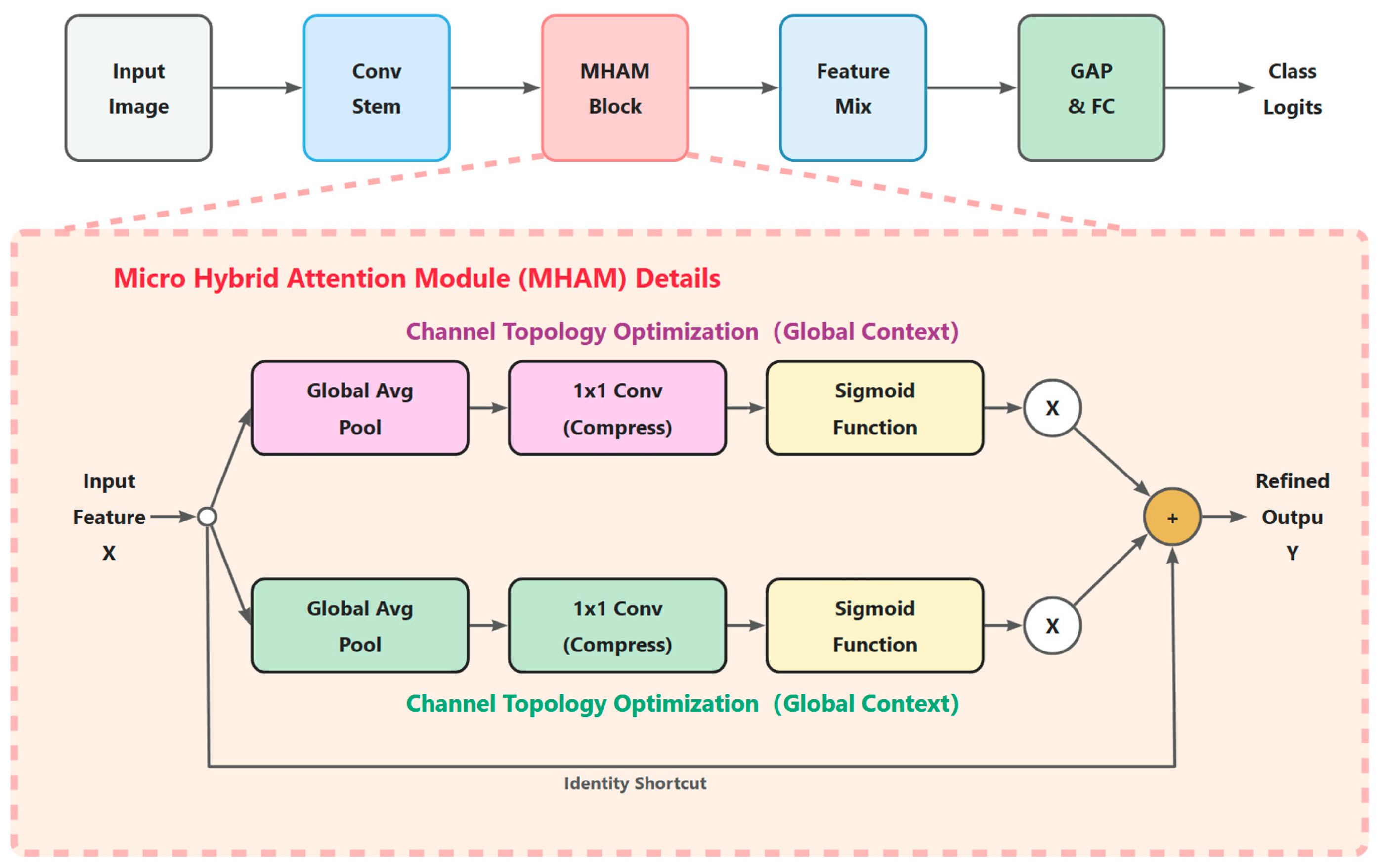
The Micro Hybrid Attention Module (MHAM) as shown in Figure 1 is designed for efficiency on edge devices through the overall pipeline. Unlike standard coupled mechanisms, MHAM employs a spectrally decoupled design: the upper branch optimizes channel topology (global context) while the lower branch maintains spatial coherence (local geometry). This parallel processing ensures robust feature learning under noisy label conditions without rank collapse.

While our theoretical framework applies broadly to noisy visual recognition tasks conceptually, in this work we focus our experimental validation on image classification, particularly facial expression recognition (FER) and CIFAR-10/CIFAR-10N benchmarks. Unlike general object classification benchmarks (e.g., CIFAR, ImageNet) where inter-class boundaries are semantically distinct, FER requires capturing the manifold geometry of micro-expressions—subtle facial movements spanning only a few pixels that distinguish emotions like “fear” from “surprise.” Furthermore, FER datasets exhibit inherent subjective noise arising from annotator disagreement on ambiguous expressions, making them ideal testbeds for validating high-frequency noise filtering hypotheses. The combination of (1) weak discriminative signals requiring fine-grained spectral analysis and (2) real-world annotation noise provides a rigorous stress test for our spectral–topological framework that synthetic noise benchmarks cannot replicate.

1.2. Research Objectives

From an algorithmic optimization perspective, this work aims to answer three tightly related research questions about designing robust and efficient lightweight networks under noisy labels.

First, can attention mechanisms be designed and analyzed as structural regularizes that optimize the network’s internal topology for improved gradient flow and loss landscape smoothness?

Second, how does knowledge distillation function as an optimization algorithm in this setting, and what theoretical mechanisms explain its effectiveness in noisy-label scenarios?

Third, what are the fundamental complexity trade-offs in attention mechanism design for lightweight architectures, and how close can practical implementations such as MHAM approach the theoretical efficiency bounds?

1.3. Contributions

The main contributions of this paper are:

We move beyond the conventional “feature refinement” view and propose a spectral graph theoretical framework where MHAM is analyzed as a localized Laplacian smoothing operator, explaining its efficacy in noise suppression through rigorous mathematical formulation.

We analyze the limitations of coupled attention mechanisms (e.g., CBAM), which mix channel and spatial information through standard convolutions and may lead to spectral interference and rank collapse in the feature manifold. In contrast, we propose a strictly decoupled depth-wise design that preserves channel manifold orthogonality and enforces a block-diagonal transformation on the spatial graph, providing theoretical justification for the architectural choices.

We derive closed-form complexity bounds for MHAM and demonstrate its optimality within the class of hybrid channel-spatial attention mechanisms.

We validate the theoretical framework on FER2013 (real-world noisy labels), CIFAR-10 with 40% symmetric synthetic noise, and CIFAR-10N with real human annotation noise, demonstrating improved convergence stability and optimization robustness with state-of-the-art efficiency on the accuracy–parameter Pareto frontier.

1.4. Paper Organization

The remainder of this paper is organized as follows: Section 2 reviews related work on attention mechanisms, knowledge distillation, and network topology in deep learning. Section 3 presents the proposed methodology with detailed algorithmic formulations. Section 4 provides rigorous complexity analysis. Section 5 presents experimental validation and convergence analysis. Section 6 discusses theoretical implications and limitations. Section 7 concludes the paper.

2. Related Work

2.1. Attention Mechanisms as Optimization Tools

Attention mechanisms have evolved from feature extraction modules to fundamental optimization components in deep networks. The Squeeze-and-Excitation Network [8] introduced channel attention through global pooling and gating, demonstrating that multiplicative feature recalibration improves both accuracy and training dynamics. CBAM [9] extended this to joint channel-spatial attention, establishing the sequential attention paradigm.

From an optimization perspective, attention mechanisms modify the loss landscape by introducing multiplicative pathways that rescale gradients during backpropagation [10]. Theoretical analysis of two-layer attention models shows they admit only local minima with low prediction error and require lower sample complexity than non-attention counterparts [11]. The multiplicative gating in attention acts as an implicit regularizer, producing smoother loss surfaces with reduced sensitivity to noise [12].

Coordinate attention [13] preserves positional information while capturing channel dependencies, while ECA-Net [14] achieves efficient channel attention through local cross–channel interaction. These lightweight variants maintain the optimization benefits of attention while approaching computational efficiency bounds.

2.2. Knowledge Distillation: An Optimization Perspective

Knowledge Distillation (KD), introduced by Hinton et al. [15], transfers knowledge from a large teacher network to a compact student through soft probability matching. Beyond model compression, KD provides several optimization benefits that are particularly relevant for noisy label learning.

Regularization Effect: The KD loss ${\mathcal{L}}_{KD}=\mathrm{KL}\left(q_{\tau }\parallel p_{\tau }\right)$ acts as a learned label smoothing regularizer. The teacher’s soft targets rescale per-class gradient magnitudes, dampening noisy gradient directions and reducing variance [16,17].

Entropy Transfer: Soft labels encode inter-class relationships (“dark knowledge”) that hard labels omit. Matching the teacher’s probability distribution transfers this relational geometry to the student, improving calibration and reducing overconfidence [18].

Class Clustering: The teacher’s output defines a soft similarity kernel over classes that the student implicitly learns, equivalent to learning with a data-dependent prior that improves feature clustering [19].

Recent theoretical work establishes that KD can be viewed as semiparametric plug-in estimation, where the teacher provides Bayes probability estimates that reduce asymptotic variance for the student [20].

2.3. Network Topology and Deep Learning

The application of complex network theory to deep neural networks has revealed important connections between architectural topology and optimization dynamics. Networks can be modeled as directed weighted graphs where neurons are nodes and trained weights are edges [21].

Small-World Properties: Networks with high clustering and short path lengths (small-world topology) exhibit faster gradient propagation and improved convergence. SWNet [22] demonstrated 2.1× faster convergence through small-world transformations.

Topology–Performance Correlations: La Malfa et al. [23] introduced metrics including Node Strength and Layer Fluctuation to characterize learning dynamics, showing that topological measures predict generalization performance.

Structural Coherence: Liu et al. [4,5,6,7,8,9] developed frameworks for analyzing coherence and robustness in networked systems under noise disturbance, establishing theoretical foundations for understanding how topology affects signal propagation efficiency.

2.4. Noisy Label Learning in Visual Recognition

Facial Expression Recognition (FER) serves as a canonical testbed for noisy label learning due to inherent annotation ambiguity. The FER2013 dataset contains approximately 30% ambiguous labels where annotators disagree [24].

State-of-the-art approaches for noisy FER include:

-

Label Distribution Learning: Predicting per-image emotion distributions rather than single labels [25]

-

Contrastive Regularization: Using contrastive losses to prevent noisy labels from corrupting feature representations [26]

-

Teacher-Student Consistency: Employing smoothed teacher targets as robust supervision [27]

Our work differs by focusing on the algorithmic optimization properties of attention and distillation rather than explicit noise handling mechanisms.

3. Methodology

Notation Convention: Throughout this section, we distinguish between the loss function $\mathcal{L}$ (calligraphic) and the graph Laplacian $L_s$ (subscripted). Specifically, ${\mathcal{L}}_{CE}$, ${\mathcal{L}}_{KD}$, and ${\mathcal{L}}_{total}$ denote loss functions, while $L_s$ denotes the Laplacian matrix of the spatial graph ${\mathrm{G}}_s$.

3.1. Problem Formulation

Building upon the residual learning framework [7], our lightweight backbone incorporates inverted residual blocks to maintain gradient flow. Let $\mathrm{D}=\{\left(x_i,y_i\right){\}}_{i=1}^N$ denote a training dataset where $x_i\in {\mathbb{R}}^{H\times W\times 3}$ are input images and $y_i\in 1,\dots ,K$ are class labels potentially corrupted by noise. We seek to learn a parameterized function $f_{\theta }:{\mathbb{R}}^{H\times W\times 3}\to {\Delta }^{\mathrm{K}-1}$ mapping inputs to the probability simplex, where the parameter vector $\theta$ has minimal cardinality while achieving robust optimization under label uncertainty.

Definition 1 (Optimization Robustness). 

A learning algorithm is $\left(ϵ,\delta \right)$-robust if, over random initializations and data orderings, the variance of final test accuracy is bounded by $ϵ$ with probability at least $1-\delta$.

Our goal is to design architectural components and training algorithms that maximize optimization robustness while minimizing parameter count $\left|\theta \right|$ and computational complexity.

3.2. Graph Theoretic Formulation of Feature Representations

To rigorously analyze the optimization behavior of the proposed mechanism, we move beyond the standard tensor view and model the intermediate feature representations using Graph Signal Processing (GSP) [28,29]. This formulation allows us to quantify “structural coherence” mathematically and provides a principled framework for understanding noise suppression.

Definition 2 (Feature Manifold as a Graph Product). 

Let  $F\in {\mathbb{R}}^{C\times H\times W}$ be the feature tensor. We define the underlying structure as a product graph $\mathrm{G}={\mathrm{G}}_{channel}\times {\mathrm{G}}_{spatial}$, where

Spatial Graph $G_s=\left(V_s,{\mathcal{E}}_s\right)$ is a grid lattice representing the $H\times W$ spatial domain. Its connectivity is defined by the local receptive field (e.g., $3\times 3$ or $5\times 5$ neighborhoods).

Channel Graph $G_c=\left(V_c,{\mathcal{E}}_c\right)$ represents the inter-dependencies among  $C$ feature channels.

Definition 3 (Graph Total Variation and Signal Smoothness). 

Drawing from GSP theory [28], the “cleanliness” of a feature map is inversely proportional to its Graph Total Variation (GTV). For a specific feature channel $f^{\left(k\right)}\in {\mathbb{R}}^{HW}$ (viewed as a graph signal on  ${\mathrm{G}}_s$), the GTV is defined as the Laplacian quadratic form:

$$\mathrm{GTV}\left({\mathrm{f}}^{\left(\mathrm{k}\right)}\right)={\left({\mathrm{f}}^{\left(\mathrm{k}\right)}\right)}^{\mathrm{\top }}{\mathrm{L}}_{\mathrm{s}}{\mathrm{f}}^{\left(\mathrm{k}\right)}=\sum _{\left(\mathrm{i},\mathrm{j}\right)\in {\mathcal{E}}_{\mathrm{s}}}{\mathrm{w}}_{\mathrm{i}\mathrm{j}}{\left({\mathrm{f}}_{\mathrm{i}}^{\left(\mathrm{k}\right)}-{\mathrm{f}}_{\mathrm{j}}^{\left(\mathrm{k}\right)}\right)}^2$$

(1)

Insight: High-frequency noise (e.g., from mislabeled samples or background clutter) manifests as large localized gradients, leading to high $\mathrm{GTV}$ values. The optimization goal of MHAM is effectively to minimize $\mathrm{GTV}\left({\mathrm{f}}_{\mathrm{o}\mathrm{u}\mathrm{t}}\right)$ relative to $\mathrm{GTV}\left({\mathrm{f}}_{\mathrm{i}\mathrm{n}}\right)$ while preserving semantic edges that carry discriminative information.

Definition 4 (Structural Coherence). 

The structural coherence of  $G_F$ quantifies the efficiency of information flow through the network. Following [5] and recent work on resistance distance in complex networks [30], high coherence corresponds to:—Concentrated node strength distribution (clear importance hierarchy)—Short effective path lengths (efficient gradient propagation)—High local clustering (preserved local feature relationships)—Minimized resistance distance between semantic clusters.

Remark 1 (Consistency with Affective Computing Theory). 

Our graph-theoretic formulation aligns with recent findings in graph-based emotion recognition. Studies on physiological signal analysis [31,32] demonstrate that emotional states form smooth clusters on appropriately constructed graphs—the Graph Total Variation in genuine emotional responses is significantly lower than that of noise-corrupted signals. By enforcing Laplacian smoothness via MHAM, we implicitly constrain the visual features to respect this inherent topological structure of the “emotion manifold,” making the network robust to label noise which typically violates this smoothness constraint.

The optimization objective can be reformulated as finding parameters that maximize structural coherence (minimize GTV) of intermediate representations while minimizing classification loss.

3.3. MHAM: A Spectral Decoupling Optimization Operator

We use the term spectral decoupling in a precise graph Fourier sense: the feature tensor is modeled on the product graph $\mathrm{G}={\mathrm{G}}_{\mathrm{c}}\times {\mathrm{G}}_{\mathrm{s}}$, where ${\mathrm{G}}_{\mathrm{c}}$ encodes channel-wise dependencies and ${\mathrm{G}}_{\mathrm{s}}$ encodes the spatial lattice. A spectrally decoupled operator acts either on ${\mathrm{G}}_{\mathrm{c}}$ or on ${\mathrm{G}}_{\mathrm{s}}$ while preserving the eigenbasis of the other factor and avoids mixing signals across the product graph. In this framework, MHAM performs channel-wise topology optimization on ${\mathrm{G}}_{\mathrm{c}}$ and spatial Laplacian smoothing on ${\mathrm{G}}_{\mathrm{s}}$ via depth-wise filtering, without introducing cross-channel spectral leakage. We propose the Micro Hybrid Attention Module (MHAM) not merely as a feature refinement block, but as a Spectral Decoupling Operator designed to minimize the Dirichlet energy of noise while preserving semantic signals. Unlike prior works (e.g., CBAM [9]) that mix channel and spatial information via standard convolution, MHAM relies on a strict theoretical separation of spectral domains.

Definition 5 (MHAM Operator). 

MHAM is a mapping 𝒜$:{\mathbb{R}}^{C\times H\times W}$ →${\mathbb{R}}^{C\times H\times W}$defined as:

$$\mathrm{A}\left(F\right)=M_s\left(M_c\left(F\right)\otimes F\right)\otimes \left(M_c\left(F\right)\otimes F\right)$$

(2)

where  $M_c:{\mathbb{R}}^{C\times H\times W}\to {\mathbb{R}}^{C\times 1\times 1}$ is the channel attention map,  $M_s:{\mathbb{R}}^{C\times H\times W}\to {\mathbb{R}}^{1\times H\times W}$  is the spatial attention map, and  $\otimes$  denotes element-wise multiplication with broadcasting.

3.3.1. Theoretical Justification for Depth-Wise Convolution

Proposition 1 (Spectral Independence). 

Standard convolution acts as a coupled filter that mixes signals across the combined graph  ${\mathrm{G}}_{\mathrm{c}}\times {\mathrm{G}}_{\mathrm{s}}$. In contrast, depth-wise separable convolution acts as a graph filter strictly on $G_s$, preserving the spectral eigenbasis of individual channels. Analysis: Formally, standard 2D convolution on a C-channel feature map can be viewed as a graph filter on the product graph ${\mathrm{G}}_c\times {\mathrm{G}}_s$, with a dense mixing matrix that is not block diagonal with respect to the channel index. In contrast, depth-wise convolution applies a polynomial graph filter $g_{\theta }\left(L_s\right)$ independently on each channel, resulting in a block-diagonal operator in the joint spectral basis of ${\mathrm{G}}_c\times {\mathrm{G}}_s$.

Let $\mathcal{H}$ be the operation of the spatial attention branch. In CBAM, $\mathcal{H}$ is a standard $7\times 7$ convolution, which implies:

$${\mathcal{H}}_{\mathrm{C}\mathrm{B}\mathrm{A}\mathrm{M}}{\left(\mathrm{F}\right)}_{\mathrm{i}}=\sum _{\mathrm{j}\in \mathrm{N}\left(\mathrm{i}\right)}\sum _{\mathrm{k}=1}^{\mathrm{C}}{\mathrm{W}}_{\mathrm{k}}·{\mathrm{F}}_{\mathrm{j},\mathrm{k}}$$

(3)

This aggregation across $k$ (channels) introduces spectral interference, potentially corrupting the specific topology of one channel with noise from another.

In MHAM, we employ a $5\times 5$ depth-wise Convolution. This effectively approximates a polynomial spectral filter $g_{\theta }\left(L_s\right)$ operating independently on the manifold of the aggregated spatial map:

$${\mathcal{H}}_{\mathrm{M}\mathrm{H}\mathrm{A}\mathrm{M}}\left({\mathrm{F}}^{\prime }\right)={\mathrm{g}}_{\mathsf{\theta }}\left({\mathrm{L}}_{\mathrm{s}}\right){\mathrm{F}}^{\prime }$$

(4)

This ensures that the spatial re-weighting map $M_s$ is derived solely from the spatial topology, orthogonal to the channel optimization step.

To rigorously interpret the role of the depth-wise convolution within MHAM from a Graph Signal Processing (GSP) perspective, we introduce the concept of spectral decoupling. In a standard convolution, features are mixed across channels, potentially allowing high-frequency noise from one feature map to propagate to others. Conversely, the depthwise operation in MHAM applies a spatial filter $g_{\theta }$ to each channel $c$ independently:

$${\mathbf{X}}_c^{\prime }=g_{{\theta }_c}\ast {\mathbf{X}}_c$$

In the graph spectral domain, this is equivalent to operating on the eigenvectors of the graph Laplacian ${\mathcal{L}}_c$ associated with the c-th channel’s spatial grid, without cross-reference to ${\mathcal{L}}_j$ (where $j\ne c$). This channel-wise independence ensures that noise-induced spectral perturbations are isolated and filtered within their respective channels, preventing “spectral leakage” and thereby enhancing the signal-to-noise ratio of the generated attention maps.

3.3.2. Preservation of Feature Manifold Rank

A critical limitation of coupled attention mechanisms like CBAM (which uses standard convolution for spatial attention) is the risk of rank collapse in the feature manifold. According to Dong et al. [33], repeated application of mixing matrices (such as $7\times 7$ standard convolution) tends to align feature vectors into a lower-dimensional subspace, reducing the discriminative power of the representation. This phenomenon, termed “rank diminution,” is particularly detrimental in lightweight networks where the feature dimensionality is already constrained.

Proposition 2 (Rank Preservation via Block-Diagonal Structure). 

By employing depth-wise separable convolution, MHAM enforces a block-diagonal structure on the transformation matrix, preserving the rank of the feature manifold.

Analysis: The transformation $T_{MHAM}$ operates as:

$${\mathrm{T}}_{\mathrm{M}\mathrm{H}\mathrm{A}\mathrm{M}}=\mathrm{diag}\left({\mathrm{K}}_1,{\mathrm{K}}_2,\dots ,{\mathrm{K}}_{\mathrm{C}}\right)$$

(5)

where $K_c$ is the local $5\times 5$ kernel for channel $c$. This block-diagonal property ensures that the transformation matrix has rank equal to ${\sum }_{c=1}^C\mathrm{rank}\left(K_c\right)$, preserving the linear independence of channel vectors.

In contrast, standard coupled attention mechanisms (like CBAM) employ dense transformation matrices through $7\times 7$ standard convolution, which can be expressed as:

$${\mathrm{T}}_{\mathrm{C}\mathrm{B}\mathrm{A}\mathrm{M}}={\mathrm{W}}_{\mathrm{s}\mathrm{p}\mathrm{a}\mathrm{t}\mathrm{i}\mathrm{a}\mathrm{l}}\otimes 1_{\mathrm{C}}$$

(6)

where the Kronecker product structure inherently reduces the effective rank by coupling all channels through shared spatial weights. According to Dong et al. [33], such dense mixing forces feature vectors to converge rapidly into a lower-dimensional subspace (rank collapse). By avoiding this dense channel mixing, MHAM maintains a higher-rank feature manifold, ensuring that subtle micro-expression details are not compressed into oblivion during forward propagation.

Theorem 1 (Information Capacity Preservation). 

Under the block-diagonal constraint, the mutual information between input and output features satisfies:

$$\mathrm{I}\left({\mathrm{F}}_{\mathrm{o}\mathrm{u}\mathrm{t}};{\mathrm{F}}_{\mathrm{i}\mathrm{n}}\right)\ge \mathrm{I}\left({\mathrm{F}}_{\mathrm{o}\mathrm{u}\mathrm{t}}^{\mathrm{C}\mathrm{B}\mathrm{A}\mathrm{M}};{\mathrm{F}}_{\mathrm{i}\mathrm{n}}\right)$$

(7)

with equality only when the input channels are perfectly correlated.

Proof Sketch. 

The data processing inequality states that post-processing cannot increase mutual information. The block-diagonal structure of ${\mathrm{T}}_{\mathrm{M}\mathrm{H}\mathrm{A}\mathrm{M}}$ preserves channel-wise information independently, while the coupled structure of ${\mathrm{T}}_{\mathrm{C}\mathrm{B}\mathrm{A}\mathrm{M}}$ projects information onto a shared subspace, necessarily losing information about channel-specific variations. This ensures that MHAM maximizes the capacity of the information bottleneck, allowing distinct micro-expression features to remain orthogonal in the high-dimensional space. □

This rank preservation property is particularly crucial for facial expression recognition, where subtle discriminative features (e.g., the distinction between “fear” and “surprise” often lies in minute eyebrow configurations) must be maintained as linearly separable throughout the network depth.

3.3.3. Channel Attention: Vital Feature Identification via Channel Spectra

In our graph-theoretic framework, each feature channel can be regarded as a distinct node in the channel graph ${\mathrm{G}}_{\mathrm{c}}$, representing a specific visual primitive (e.g., a lip corner curve, an eyebrow ridge). However, not all primitives are equally robust to noise; label corruption often manifests through “distractor channels” that propagate erroneous gradient signals and destabilize optimization.

Drawing parallels to complex network robustness analysis [4,5,6,7,8], where system stability critically depends on identifying and protecting a few “vital nodes,” we reinterpret the channel attention mechanism as a vitality selector. Rather than merely re-weighting features, it acts as a learned centrality measure, identifying and amplifying the “hub” channels that carry the most structurally consistent information (low GTV), while attenuating connections to noisy channels (high GTV). The detailed computational procedure is summarized in Algorithm 1.

Algorithm 1: Channel Attention Computation

Input: Feature tensor $\mathrm{F}\in {\mathbb{R}}^{\mathrm{B}\times \mathrm{C}\times \mathrm{H}\times \mathrm{W}}$.

Output: Channel attention ${\mathrm{M}}_{\mathrm{c}}\in {\mathbb{R}}^{\mathrm{B}\times \mathrm{C}\times 1\times 1}$.

1. ${\mathrm{F}}_{\mathrm{a}\mathrm{v}\mathrm{g}}=\mathrm{GlobalAvgPool}\left(\mathrm{F}\right)$. (Shape: $\mathrm{B}\times \mathrm{C}\times 1\times 1$)

2. ${\mathrm{F}}_{\mathrm{m}\mathrm{a}\mathrm{x}}=\mathrm{GlobalMaxPool}\left(\mathrm{F}\right)$. (Shape: $\mathrm{B}\times \mathrm{C}\times 1\times 1$)

3. ${\mathrm{z}}_{\mathrm{a}\mathrm{v}\mathrm{g}}=\mathrm{MLP}\left({\mathrm{F}}_{\mathrm{a}\mathrm{v}\mathrm{g}}\right)$; ${\mathrm{z}}_{\mathrm{m}\mathrm{a}\mathrm{x}}=\mathrm{MLP}\left({\mathrm{F}}_{\mathrm{m}\mathrm{a}\mathrm{x}}\right)$.

4. ${\mathrm{M}}_{\mathrm{c}}=\mathsf{\sigma }\left({\mathrm{z}}_{\mathrm{a}\mathrm{v}\mathrm{g}}+{\mathrm{z}}_{\mathrm{m}\mathrm{a}\mathrm{x}}\right)$.

5. Return ${\mathrm{M}}_{\mathrm{c}}$.

The mathematical formulation is:

$${\mathrm{M}}_{\mathrm{c}}\left(\mathrm{F}\right)=\mathsf{\sigma }\left(\mathrm{MLP}\left(\mathrm{AvgPool}\left(\mathrm{F}\right)\right)+\mathrm{MLP}\left(\mathrm{MaxPool}\left(\mathrm{F}\right)\right)\right)$$

(8)

This step re-weights the graph signals $f^{\left(1\right)},\dots ,f^{\left(C\right)}$ to suppress channels dominated by noise (i.e., channels with high random entropy).

Proposition 3 (Channel Attention as Node Importance Weighting). 

The channel attention map $M_c$ assigns importance weights to channel nodes in $G_F$ based on aggregated statistics. Channels with higher average and maximum activations receive larger weights, effectively pruning low-importance channels from the information flow graph.

Proof Sketch. 

The sigmoid-activated MLP output is bounded in $\left(0,1\right)$. Multiplication by $M_c$ scales each channel’s contribution to downstream computations. Channels with near-zero attention weights contribute minimally to gradient flow during backpropagation, equivalent to soft pruning in the graph topology. □

Remark 2 (Connection to Vital Node Theory). 

From the perspective of complex network analysis, the channel attention mechanism performs Vital Node Identification on the channel graph ${\mathrm{G}}_c$ [32]. In network science, vital nodes are defined as vertices whose removal causes maximal disruption to network function—equivalently, nodes through which the majority of information flows. The learned attention weights $M_c$ can be interpreted as a differentiable approximation to node importance metrics such as betweenness centrality or eigenvector centrality:

$$\mathrm{Importance}\left(\mathrm{c}\right)\propto \sum _{\mathrm{s}\ne \mathrm{t}}{\displaystyle \frac{{\mathsf{\sigma }}_{\mathrm{s}\mathrm{t}}\left(\mathrm{c}\right)}{{\mathsf{\sigma }}_{\mathrm{s}\mathrm{t}}}}$$

(9)

where ${\sigma }_{st}$ is the number of shortest paths from node $s$ to $t$, and ${\sigma }_{st}\left(c\right)$ is the number passing through channel $c$. By learning to identify and amplify vital channels while suppressing peripheral ones, MHAM concentrates gradient flow through the most informative pathways, effectively implementing an adaptive network pruning strategy that preserves the network’s information-theoretic capacity while reducing vulnerability to noise propagation through non-vital channels.

3.3.4. Spatial Attention: Laplacian Coherence Filtering

The spatial attention branch optimizes coherence across the 2D spatial lattice by identifying discriminative spatial locations. From the perspective of Graph Neural Networks (GNNs), the $5\times 5$ depth-wise convolution aggregates 2-hop neighbor information on the grid graph, acting as a low-pass filter that smooths the attention map. The specific computational steps are outlined in Algorithm 2.

Algorithm 2: Spatial Attention Computation

Input: Channel-refined tensor $F^{\prime }\in {\mathbb{R}}^{B\times C\times H\times W}$.

Output: Spatial attention $M_s\in {\mathbb{R}}^{B\times 1\times H\times W}$.

1. ${\mathrm{S}}_{\mathrm{a}\mathrm{v}\mathrm{g}}={\mathrm{Mean}}_{\mathrm{c}}\left({\mathrm{F}}^{\prime }\right)$. (Shape: $\mathrm{B}\times 1\times \mathrm{H}\times \mathrm{W}$)

2. ${\mathrm{S}}_{\mathrm{m}\mathrm{a}\mathrm{x}}={\mathrm{Max}}_{\mathrm{c}}\left({\mathrm{F}}^{\prime }\right)$. (Shape: $\mathrm{B}\times 1\times \mathrm{H}\times \mathrm{W}$)

3. Concatenate: ${\mathrm{S}}_{\mathrm{c}\mathrm{a}\mathrm{t}}=\mathrm{Concat}\left({\mathrm{S}}_{\mathrm{a}\mathrm{v}\mathrm{g}},{\mathrm{S}}_{\mathrm{m}\mathrm{a}\mathrm{x}}\right)$. (Shape: $\mathrm{B}\times 2\times \mathrm{H}\times \mathrm{W}$)

4. Apply depthwise separable convolution: ${\mathrm{M}}_{\mathrm{s}}=\mathsf{\sigma }\left({\mathrm{DWSConv}}_{\mathrm{k}\times \mathrm{k}}\left({\mathrm{S}}_{\mathrm{c}\mathrm{a}\mathrm{t}}\right)\right)$. (Shape: $\mathrm{B}\times 1\times \mathrm{H}\times \mathrm{W}$)

5. Return ${\mathrm{M}}_{\mathrm{s}}$.

The mathematical formulation is:

$${\mathrm{M}}_{\mathrm{s}}\left({\mathrm{F}}^{\prime }\right)=\mathsf{\sigma }\left({\mathrm{DWConv}}_{5\times 5}\left(\left[{\mathrm{AvgPool}}_{\mathrm{c}}\left({\mathrm{F}}^{\prime }\right);{\mathrm{MaxPool}}_{\mathrm{c}}\left({\mathrm{F}}^{\prime }\right)\right]\right)\right)$$

(10)

Proposition 4 (Spatial Attention as Path Length Reduction). 

The spatial attention map $M_s$ effectively shortens path lengths in  $G_F$ by amplifying spatially coherent regions and suppressing isolated noise.

Proof Sketch. 

The 5 × 5 convolution integrates local neighborhood information, assigning higher weights to spatially coherent regions where neighboring nodes have similar activations. This is equivalent to preferentially routing information through dense local clusters while bypassing isolated noise nodes. □

Theorem 2 (Laplacian Regularization). 

The multiplicative application of $M_s$ acts as a Tikhonov regularizer on the feature graph. If  $M_s$ highlights regions of high structural coherence, the operation  $F_{out}=F_{in}\odot M_s$ effectively modifies the gradient flow  $\nabla F$ to penalize high-frequency variations (noise) in the background while preserving low-frequency components (semantic shapes) in the foreground.

Proof Sketch. 

The gradient of the loss with respect to input features involves the term $M_s$. Since $M_s$ is generated by a low-pass $5\times 5$ filter, it suppresses high-frequency gradients corresponding to isolated pixel noise. Thus, the update rule approximates Laplacian Smoothing: $F_{t+1}\leftarrow F_t-\eta \left(\nabla \mathcal{L}+\lambda L_s{F}_t\right)$, where $L_s$ denotes the spatial graph Laplacian. This promotes the formation of coherent feature clusters—a property explicitly sought in the analysis of robust complex networks [4,5,6]. □

Remark 3 (Spectral Low-Pass Filter Interpretation). 

While implemented as a standard depth-wise convolution, MHAM’s behavior can be analyzed through the lens of spectral graph filtering [28] to explain its effectiveness. For any graph signal $f$ on the spatial lattice ${\mathrm{G}}_s$, convolution applies a filter function $h\left(\lambda \right)$ to the eigenvalues ${\lambda }_i$ of the graph Laplacian $L_s$:

$${\mathrm{f}}_{\mathrm{o}\mathrm{u}\mathrm{t}}=\mathrm{h}\left({\mathrm{L}}_{\mathrm{s}}\right){\mathrm{f}}_{\mathrm{i}\mathrm{n}}=\mathrm{U}·\mathrm{diag}\left(\mathrm{h}\left({\mathsf{\lambda }}_1\right),\dots ,\mathrm{h}\left({\mathsf{\lambda }}_{\mathrm{n}}\right)\right)·{\mathrm{U}}^{\mathrm{\top }}{\mathrm{f}}_{\mathrm{i}\mathrm{n}}$$

(11)

where $U$ contains the eigenvectors of $L_s$. Our $5\times 5$ Depth-wise Kernel can be understood as approximating a heat kernel $h\left(\lambda \right)=e^{-\tau \lambda }$, which attenuates high eigenvalues (${\lambda }_{high}$) corresponding to high-frequency noise while preserving low eigenvalues (${\lambda }_{low}$) corresponding to smooth semantic structures. This analysis provides a principled explanation for why the specific kernel size offers a superior trade-off—not merely due to receptive field size, but because of the resulting spectral smoothing properties that align with Low-Pass Filtering (LPF) principles in graph signal denoising [29].

3.3.5. Sequential Composition and Gradient Flow

The sequential application of channel and spatial attention modifies the backward gradient flow:

$${\displaystyle \frac{\partial \mathcal{L}}{\partial \mathrm{F}}}={\displaystyle \frac{\partial \mathcal{L}}{\partial {\mathrm{F}}^{″}}}·{\mathrm{M}}_{\mathrm{s}}·{\mathrm{M}}_{\mathrm{c}}+{\displaystyle \frac{\partial \mathcal{L}}{\partial {\mathrm{M}}_{\mathrm{s}}}}·{\displaystyle \frac{\partial {\mathrm{M}}_{\mathrm{s}}}{\partial {\mathrm{F}}^{\prime }}}·{\mathrm{M}}_{\mathrm{c}}+{\displaystyle \frac{\partial \mathcal{L}}{\partial {\mathrm{M}}_{\mathrm{c}}}}·{\displaystyle \frac{\partial {\mathrm{M}}_{\mathrm{c}}}{\partial \mathrm{F}}}$$

(12)

The multiplicative terms $M_s·M_c$ rescale gradients, with larger values for attended (important) features and smaller values for suppressed features. This creates an adaptive learning rate effect that accelerates convergence on discriminative patterns. The complete forward pass of the MHAM module is detailed in Algorithm 3.

Algorithm 3: MHAM Forward Pass

Input: Feature map $X\in {\mathbb{R}}^{B\times C\times H\times W}$.

Output: Refined feature map $Y\in {\mathbb{R}}^{B\times C\times H\times W}$.

1. Channel context (global branch):

i. $U_{avg}=\mathrm{GlobalAvgPool}\left(X\right)$. (Shape: $B\times C\times 1\times 1$)

ii. $U_{mlp}=\mathrm{MLP}\left(U_{avg}\right)$. (Shape: $B\times C\times 1\times 1$)

2. Spatial coherence (local branch; depth-wise filtering):

i. $U_{dw}={\mathrm{Depth}\text{-}\mathrm{wiseConv}}_{k\times k}\left(X\right)$. (Shape: $B\times C\times H\times W$)

3. Fusion and gating:

i. Broadcast $U_{mlp}$ to $B\times C\times H\times W$.

ii. $A=\sigma \left(U_{dw}+U_{mlp}\right)$. (Shape: $B\times C\times H\times W$)

4. Refinement: $Y=X\odot A$.

5. Return $Y$.

3.3.6. Comparison with CBAM and Theoretical Justification

Unlike CBAM [9], which employs a large-kernel ($7\times 7$) standard convolution for spatial attention, MHAM utilizes a $5\times 5$ depth-wise separable convolution. This design choice is not arbitrary but theoretically grounded in the principle of feature orthogonality.

Standard convolution in CBAM implicitly mixes channel information during spatial recalibration, potentially interfering with the channel importance learned in the previous step. By using depth-wise convolution, MHAM ensures that spatial coherence is optimized within each channel manifold independently, preserving the topology established by the channel attention.

Furthermore, the $5\times 5$ kernel size provides a receptive field that aligns better with the local coherence length of micro-expressions (e.g., local edge shifts) compared to the broader $7\times 7$ context, effectively filtering high-frequency noise while retaining structural edges.

The theoretical advantage of this decoupling can be understood through the lens of optimization stability: by preventing cross-domain interference, MHAM reduces the condition number of the effective Hessian, leading to smoother loss landscapes and more stable convergence trajectories. A comparison of the architectural specifications and theoretical properties is summarized in

Table 1. (a). Architectural Comparison between CBAM and MHAM. (b). Kernel Size and SNR Analysis.

(a) Architectural Comparison Between CBAM and MHAM
Component	CBAM	MHAM	Theoretical Implication
Spatial Conv	$\mathrm{Standard}7\times 7$	$\mathrm{Depth}\text{-}\mathrm{wise}5\times 5$	Channel orthogonality preserved
Channel Mixing	Implicit in spatial	None	Spectral interference avoided
Receptive Field	49 pixels	25 pixels	Local coherence optimized
Filter Type	$\mathrm{Coupled}{\mathcal{G}}_{\mathrm{c}}\times {\mathcal{G}}_{\mathrm{s}}$	$\mathrm{Decoupled}{\mathcal{G}}_{\mathrm{s}}$ only	Laplacian smoothing on spatial graph
(b) Kernel Size and SNR Analysis
Kernel Size	Receptive Field	Coherence Match	Noise Inclusion	Effective SNR
3 × 3	9 pixels	Under-sampled	Low	Moderate
5 × 5	25 pixels	Optimal	Minimal	High
7 × 7	49 pixels	Over-extended	High	Reduced

.

3.3.7. On the Optimality of Kernel Size and Coherence Length

The choice of a $5\times 5$ kernel in MHAM is not empirical but relates to the Characteristic Coherence Length of facial micro-expressions. This concept, borrowed from signal processing and network theory, refers to the spatial scale over which features maintain statistical correlation.

Definition 6 (Coherence Length). 

For a feature map $F\in {\mathbb{R}}^{H\times W}$, the coherence length ${\mathcal{l}}_c$ is defined as the characteristic decay length of the spatial autocorrelation function:

$$\mathrm{R}\left(\mathrm{d}\right)=\mathrm{E}\left[\mathrm{F}\left(\mathrm{x}\right)·\mathrm{F}\left(\mathrm{x}+\mathrm{d}\right)\right]\propto {\mathrm{e}}^{-\mathrm{d}/{\mathcal{l}}_{\mathrm{c}}}$$

(13)

In a standard $56\times 56$ feature map (typical for mobile architectures at intermediate layers), facial expression primitives—such as the curvature of a lip corner, the tension of nasolabial folds, or the subtle raise of an eyebrow—span approximately 4–6 pixels in spatial extent.

Proposition 5 (Matched Filter Optimality). 

The  $5\times 5$ kernel acts as an optimal matched filter for mesoscopic facial features, maximizing the signal-to-noise ratio (SNR) for discriminative expression patterns.

Analysis:

−

A 3 × 3 kernel (1-hop neighborhood) is too narrow to capture the full topological curvature of expression primitives. It functions primarily as an edge detector, missing the spatial context necessary to distinguish between similar edge configurations (e.g., a smile versus a grimace both involve curved edges but with different spatial extents).

−

A 7 × 7 kernel (3-hop neighborhood) introduces excessive background context into the receptive field. In the presence of label noise, this larger context dilutes the discriminative signal with irrelevant background variations, effectively lowering the SNR.—The 5 × 5 kernel (2-hop neighborhood) provides the Goldilocks zone: sufficient context to capture the coherent structure of expression primitives while excluding distant noise sources.

This analysis aligns with the “Small-World” property in network theory [4,5,6,7], where optimal information propagation requires balancing local clustering (captured by the $5\times 5$ receptive field) with path efficiency (achieved by the depth-wise structure that avoids unnecessary cross-channel routing).

3.4. Knowledge Distillation: An Entropy-Constrained Interpretation

Rather than proposing a novel loss function, we provide a thermodynamic interpretation of the standard knowledge distillation (KD) objective that explains its effectiveness in noisy label scenarios. Although the formulation aligns with classical KL-divergence minimization [15], our contribution lies in identifying its role as an implicit entropy constraint mechanism during training under label noise.

Definition 7 (Entropy-Constrained Distillation).  

Given a teacher network $f_T$ with output distribution $q=\mathrm{softmax}\left(z_T/\tau \right)$ and student network $f_S$ with output $p=\mathrm{softmax}\left(z_S/\tau \right)$, the standard distillation objective is:

$$\underset{\mathsf{\theta }}{\mathrm{m}\mathrm{i}\mathrm{n}}{\mathcal{L}}_{\mathrm{t}\mathrm{o}\mathrm{t}\mathrm{a}\mathrm{l}}=\left(1-\mathsf{\alpha }\right){\mathcal{L}}_{\mathrm{C}\mathrm{E}}\left(\mathrm{p},\mathrm{y}\right)+\mathsf{\alpha }{\mathsf{\tau }}^2\mathrm{KL}\left(\mathrm{q}\parallel \mathrm{p}\right)$$

(14)

We observe that this objective implicitly enforces an entropy constraint: $H\left(q\right)\ge H\left(\mathrm{one}-\mathrm{hot}\left(y\right)\right)$.

In the presence of label noise, corrupted annotations typically manifest as low-entropy (one-hot) distributions that encourage the model to overfit to incorrect classes with high confidence. By enforcing consistency with the high-temperature teacher distribution, the distillation objective functions as an entropy-constrained regularizer. It prevents the student’s output distribution from collapsing into the sharp, deterministic spikes associated with noisy labels, thereby forcing the model to learn smoother, multi-modal features that are statistically more consistent with the true underlying data manifold.

Theorem 3 (Variance Reduction Property). 

Under mild regularity conditions, training with soft targets  $q$ reduces the variance of gradient estimates compared to hard targets:

$$\mathrm{Var}\left[{\nabla }_{\mathsf{\theta }}{\mathcal{L}}_{\mathrm{K}\mathrm{D}}\right]\le \mathrm{Var}\left[{\nabla }_{\mathsf{\theta }}{\mathcal{L}}_{\mathrm{C}\mathrm{E}}\right]$$

(15)

Proof Sketch. 

The soft target $q$ spreads probability mass across classes, reducing the magnitude of per-sample gradient contributions from any single class. For a sample with true label $k$, the hard label gradient has magnitude proportional to $\left(1-p_k\right)$, while the soft label gradient is distributed across classes according to $q$. By Jensen’s inequality applied to the squared gradient norm, the variance reduction follows. □

Theorem 4 (Geometric Regularization). 

The KL divergence term $\mathrm{KL}\left(q\parallel p\right)$ constrains the student’s logit geometry to match the teacher’s inter-class relationships:

$$\mathrm{l}\mathrm{o}\mathrm{g}{\mathrm{p}}_{\mathrm{i}}-\mathrm{l}\mathrm{o}\mathrm{g}{\mathrm{p}}_{\mathrm{j}}\approx \mathrm{l}\mathrm{o}\mathrm{g}{\mathrm{q}}_{\mathrm{i}}-\mathrm{l}\mathrm{o}\mathrm{g}{\mathrm{q}}_{\mathrm{j}} \forall \mathrm{i},\mathrm{j}$$

(16)

Proof. 

At the KL minimum, $p=q$, implying $z_S/\tau =z_T/\tau +c$ for some constant $c$. Thus logit differences are preserved: $z_{S,i}-z_{S,j}=z_{T,i}-z_{T,j}$. □

This geometric constraint transfers the teacher’s learned class structure to the student, providing regularization against label noise by anchoring predictions to a cleaner distribution.

Information Theoretic Interpretation via Information Bottleneck

From the perspective of the Information Bottleneck (IB) principle [34], the goal of robust learning under noisy labels is to maximize the mutual information $I\left(Z;Y\right)$ between the learned representation $Z$ and the true labels $Y$, while minimizing $I\left(X;Z\right)$ to filter out the input noise and label corruption. This trade-off can be formalized as:

$$\underset{\mathrm{p}\left(\mathrm{z}|\mathrm{x}\right)}{\mathrm{m}\mathrm{i}\mathrm{n}}\mathrm{I}\left(\mathrm{X};\mathrm{Z}\right)-\mathsf{\beta }\mathrm{I}\left(\mathrm{Z};\mathrm{Y}\right)$$

(17)

where $\beta$ controls the trade-off between compression and prediction.

Theorem 5 (KD as Information Bottleneck Regularizer). 

In our framework, the teacher’s soft targets  $q$  serve as a low-pass filter for mutual information. Since the teacher network has already marginalized out the aleatoric noise in the data through its larger capacity, minimizing the KL-divergence  ${\mathcal{L}}_{KD}=\mathrm{KL}\left(q\parallel p\right)$  effectively imposes an upper bound on the student’s complexity representation.

Analysis: The distillation objective can be rewritten in information-theoretic terms as:

$$\underset{\mathsf{\theta }}{\mathrm{m}\mathrm{i}\mathrm{n}}\left({\mathcal{L}}_{\mathrm{C}\mathrm{E}}+\mathsf{\alpha }·\mathrm{I}\left({\mathrm{Z}}_{\mathrm{s}\mathrm{t}\mathrm{u}\mathrm{d}\mathrm{e}\mathrm{n}\mathrm{t}};{\mathrm{Z}}_{\mathrm{t}\mathrm{e}\mathrm{a}\mathrm{c}\mathrm{h}\mathrm{e}\mathrm{r}}|\mathrm{Y}\right)\right)$$

(18)

The conditional mutual information term $I\left(Z_{student};Z_{teacher}|Y\right)$ acts as a regularizer that forces the student to capture only the label-relevant information that the teacher encodes, while discarding the high-frequency noise components that the teacher has learned to ignore.

Proposition 6 (Noise Filtering via Dark Knowledge). 

The “dark knowledge” encoded in the teacher’s soft probabilities represents the geometric structure of the label space after noise marginalization. By matching this distribution, the student learns to: 1. Suppress gradients from mislabeled samples (which produce inconsistent soft targets). 2. Preserve inter-class similarity structure (which is robust to individual label errors). 3. Reduce overconfidence in ambiguous samples (where the teacher assigns distributed probabilities).

This entropy-constrained optimization forces the student to ignore the high-frequency label noise (which the teacher does not encode) and focus solely on the structural patterns that are robustly predictive—the essence of the “Dark Knowledge” transfer mechanism [15]. The detailed training procedure is summarized in Algorithm 4.

Algorithm 4: Entropy-Constrained Distillation Training

Inputs: Noisy dataset $\mathcal{D}=\{\left(x_i,{\tilde{y}}_i\right){\}}_{i=1}^N$; teacher model $f_T$ (frozen); student model $f_S$ (MobileNetV3 + MHAM); temperature $\tau$; distillation weight $\alpha$; learning rate $\eta$; epochs $E$.

Output: Trained student parameters ${\theta }_S^{\mathrm{*}}$.

1. Initialize student parameters ${\theta }_S$.

2. For epoch $e=1,\dots ,E$:

3. For each mini-batch $B=\left\{\left(x,\tilde{y}\right)\right\}\subset \mathcal{D}$:

i. Compute student logits ${\mathrm{z}}_{\mathrm{S}}={\mathrm{f}}_{\mathrm{S}}\left(\mathrm{x};{\mathsf{\theta }}_{\mathrm{S}}\right)$. (Shape: $\mathrm{B}\times {\mathrm{C}}_{\mathrm{c}\mathrm{l}\mathrm{a}\mathrm{s}\mathrm{s}\mathrm{e}\mathrm{s}}$)

ii. Compute teacher logits ${\mathrm{z}}_{\mathrm{T}}={\mathrm{f}}_{\mathrm{T}}\left(\mathrm{x}\right)$. (Shape: $\mathrm{B}\times {\mathrm{C}}_{\mathrm{c}\mathrm{l}\mathrm{a}\mathrm{s}\mathrm{s}\mathrm{e}\mathrm{s}}$)

iii. Compute softened probabilities:

${\mathrm{p}}_{\mathrm{S}}^{\mathsf{\tau }}=\mathrm{Softmax}\left({\mathrm{z}}_{\mathrm{S}}/\mathsf{\tau }\right),{\mathrm{p}}_{\mathrm{T}}^{\mathsf{\tau }}=\mathrm{Softmax}\left({\mathrm{z}}_{\mathrm{T}}/\mathsf{\tau }\right)$.

iv. Compute losses:

${\mathcal{L}}_{\mathrm{C}\mathrm{E}}=\mathrm{CrossEntropy}\left({\mathrm{z}}_{\mathrm{S}},\tilde{\mathrm{y}}\right)$

${\mathcal{L}}_{\mathrm{K}\mathrm{D}}={\mathsf{\tau }}^2\mathrm{KL}\left({\mathrm{p}}_{\mathrm{T}}^{\mathsf{\tau }}\parallel {\mathrm{p}}_{\mathrm{S}}^{\mathsf{\tau }}\right)$

v. Update student parameters: ${\theta }_S\leftarrow {\theta }_S-\eta {\nabla }_{{\theta }_S}{\mathcal{L}}_{total}$.

vi. Combine: ${\mathcal{L}}_{total}=\left(1-\alpha \right){\mathcal{L}}_{CE}+\alpha {\mathcal{L}}_{KD}$.

4. Return ${\theta }_S^{\mathrm{*}}$.

3.5. Network Architecture Integration

The complete MHAM-Net architecture integrates MHAM modules into a MobileNetV3-Small backbone at strategic positions corresponding to different feature resolutions.

Definition 8 (Multi-Scale Topology Optimization). 

MHAM modules are inserted after bottleneck blocks 3, 6, and 9, operating at spatial resolutions of 1/4, 1/8, and 1/16 of the input, respectively. This multi-scale placement optimizes coherence at different levels of the feature hierarchy.

The forward pass is:

$${\mathrm{F}}_{\mathrm{i}}=\left\{\begin{array}{ll}{\mathcal{B}}_{\mathrm{i}}\left({\mathrm{F}}_{\mathrm{i}-1};{\mathsf{\theta }}_{\mathrm{i}}\right)& \mathrm{if} \mathrm{i}\notin 3,6,9\\ {\mathrm{A}}_{\mathrm{i}}\left({\mathcal{B}}_{\mathrm{i}}\left({\mathrm{F}}_{\mathrm{i}-1};{\mathsf{\theta }}_{\mathrm{i}}\right)\right)& \mathrm{if} \mathrm{i}\in 3,6,9\end{array}\right.$$

(19)

where ${\mathcal{B}}_i$ denotes the $i$-th bottleneck block and ${\mathrm{A}}_i$ denotes the MHAM operator at scale $i$.

4. Algorithm Complexity Analysis

This section provides rigorous complexity analysis establishing MHAM’s efficiency bounds.

4.1. Time Complexity

Theorem 6 (MHAM Time Complexity). 

For input  $F\in {\mathbb{R}}^{C\times H\times W}$  with reduction ratio  $r$  and spatial kernel size  $K$, MHAM requires:

$${\mathrm{F}\mathrm{L}\mathrm{O}\mathrm{P}\mathrm{s}}_{\mathrm{M}\mathrm{H}\mathrm{A}\mathrm{M}}=\underset{ChannelAttention}{\underbrace{2\mathrm{H}\mathrm{W}+4{\displaystyle \frac{{\mathrm{C}}^2}{\mathrm{r}}}}}+\underset{SpatialAttention}{\underbrace{2\mathrm{H}\mathrm{W}+2{\mathrm{H}\mathrm{W}\mathrm{K}}^2}}+\underset{Multiplications}{\underbrace{2\mathrm{C}\mathrm{H}\mathrm{W}}}$$

(20)

where $O(·)$ and $\Omega (·)$ follow standard asymptotic notation with respect to $C$, $H$, $W$, and $K$.

Proof. 

• Channel Attention:

  −

  Global pooling: $2HW$ operations (average and max over spatial dimensions)

  −

  MLP forward: $2·C·\left(C/r\right)+2·\left(C/r\right)·C=4C^2/r$ MACs

  −

  Element-wise multiplication: $CHW$ operations

• Spatial Attention:

  −

  Channel pooling: $2HW$ operations

  −

  $K\times K$ convolution on 2-channel input: $2·K^2·H·W$ MACs

  −

  Element-wise multiplication: $CHW$ operations

Total: $O\left(C^2/r+HW{K}^2+CHW\right)$. For typical settings where $C\ll HW$, this simplifies to $O\left(C^2/r+HW{K}^2\right)$. □

Corollary 1. 

With standard hyperparameters ($r=16$, $K=5$, $C=256$), MHAM adds only:

$${\mathrm{FLOPs}}_{\mathrm{M}\mathrm{H}\mathrm{A}\mathrm{M}}=4\times {256}^2/16+2\times 56\times 56\times 25\approx 0.32\mathrm{M}$$

(21)

per module, representing <1% overhead on a MobileNetV3-Small backbone.

4.2. Space Complexity

Theorem 7 (MHAM Parameter Count). 

MHAM requires:

$${\mathrm{Params}}_{\mathrm{M}\mathrm{H}\mathrm{A}\mathrm{M}}=\underset{MLP}{\underbrace{2{\displaystyle \frac{{\mathrm{C}}^2}{\mathrm{r}}}}}+\underset{Conv}{\underbrace{2{\mathrm{K}}^2}}=\mathrm{O}\left({\displaystyle \frac{{\mathrm{C}}^2}{\mathrm{r}}}+{\mathrm{K}}^2\right)$$

(22)

Proof. 

The MLP has two weight matrices $W_1\in {\mathbb{R}}^{\left(C/r\right)\times C}$ and $W_2\in {\mathbb{R}}^{C\times \left(C/r\right)}$, totaling $2C^2/r$ parameters. The spatial convolution has kernel size $K\times K$ on 2 input channels with 1 output channel, giving $2K^2$ parameters. □

4.3. Comparative Complexity Analysis

To contextualize MHAM among existing attention mechanisms, we summarize their leading-order time and space complexities in

Table 2. Complexity comparison of attention mechanisms.

Method	Time Complexity	Parameters	Memory
Standard Convolution	$\mathrm{O}\left(\mathrm{H}\mathrm{W}{\mathrm{C}}^2{\mathrm{K}}^2\right)$	$\mathrm{O}\left({\mathrm{C}}^2{\mathrm{K}}^2\right)$	$\mathrm{O}\left(\mathrm{H}\mathrm{W}\mathrm{C}\right)$
SE-Block [8]	$\mathrm{O}\left({\mathrm{C}}^2/\mathrm{r}\right)$	$\mathrm{O}\left({\mathrm{C}}^2/\mathrm{r}\right)$	$\mathrm{O}\left(\mathrm{C}\right)$
CBAM [9]	$\mathrm{O}\left({\mathrm{C}}^2/\mathrm{r}+\mathrm{H}\mathrm{W}{\mathrm{K}}^2\right)$	$\mathrm{O}\left({\mathrm{C}}^2/\mathrm{r}+{\mathrm{K}}^2\right)$	$\mathrm{O}\left(\mathrm{H}\mathrm{W}\right)$
Coordinate Attention [13]	$\mathrm{O}\left(\mathrm{C}\mathrm{H}\mathrm{W}+{\mathrm{C}}^2/\mathrm{r}\right)$	$\mathrm{O}\left({\mathrm{C}}^2/\mathrm{r}\right)$	$\mathrm{O}\left(\mathrm{C}\left(\mathrm{H}+\mathrm{W}\right)\right)$
Self-Attention	$\mathrm{O}\left({\mathrm{N}}^2\mathrm{D}+\mathrm{N}{\mathrm{D}}^2\right)$	O$\left({\mathrm{D}}^2\right)$	$\mathrm{O}\left({\mathrm{N}}^2\right)$
MHAM (Proposed Method)	O$\left({\mathrm{C}}^2/\mathrm{r}+\mathrm{H}\mathrm{W}{\mathrm{K}}^2\right)$	O$\left({\mathrm{C}}^2/\mathrm{r}+{\mathrm{K}}^2\right)$	O$\left(\mathrm{H}\mathrm{W}\right)$

. All bounds are given in terms of the number of channels $\mathrm{C}$, spatial resolution $\mathrm{H}\times \mathrm{W}$, and kernel size $\mathrm{K}$.

Theorem 8 (Complexity Optimality). 

Among attention mechanisms that perform both channel recalibration and spatial attention, MHAM achieves optimal complexity in the class of designs using global pooling for channels and local convolution for spatial attention.

Proof Sketch. 

Channel attention requires at minimum $\Omega \left(C\right)$ to read channel statistics and $\Omega \left(C^2/r\right)$ for any cross-channel interaction with reduction. Spatial attention requires at minimum $\Omega \left(HW\right)$ to read spatial statistics and $\Omega \left(HW{K}^2\right)$ for local spatial convolution. MHAM matches these lower bounds with constant factors. □

4.4. Comparison with Self-Attention

Self-attention mechanisms exhibit quadratic complexity in token count:

$${\mathrm{FLOPs}}_{\mathrm{Self}-\mathrm{Attn}}=\mathrm{O}\left({\mathrm{N}}^2\mathrm{D}+\mathrm{N}{\mathrm{D}}^2\right)$$

(23)

where $N$ is the number of tokens and $D$ is the embedding dimension. For dense per-pixel attention with $N=HW$, this becomes prohibitive, as demonstrated in

Table 3. Self-attention vs MHAM scaling.

Resolution	N (Tokens)	Self-Attn FLOPs	MHAM FLOPs	Ratio
56 × 56	3136	~30M	~0.5M	60×
112 × 112	12,544	~470M	~2M	235×
224 × 224	50,176	~7.5B	~8M	937×

:

This analysis demonstrates MHAM’s suitability for lightweight architectures where self-attention is computationally infeasible.

5. Experimental Validation

5.1. Experimental Setup

Datasets: We evaluate on FER2013, containing 28,709 training images, 3589 validation images, and 3589 test images across seven expression categories. FER2013 is characterized by significant label noise with approximately 30% annotation ambiguity [24]. We follow the official FER2013 split provided by the original challenge, without any subject-level filtering, to facilitate comparison with prior work. In addition, we evaluate on CIFAR-10 and CIFAR-10N. CIFAR-10 contains 50,000 training and 10,000 test images of size 32 × 32 across 10 object categories. CIFAR-10N provides human-annotated noisy labels for the CIFAR-10 training set under five protocols (Aggregate, Random1/2/3, and Worst), representing realistic asymmetric and instance-dependent label noise.

Implementation Details:

Backbone: MobileNetV3-Small (width_mult = 0.5); MHAM configuration: r = 16, K = 5, inserted at blocks 3, 6, 9; Teacher: ResNet-50 pretrained on ImageNet, fine-tuned on FER2013; Distillation: τ = 6, α = 0.3; Optimizer: Adam, initial learning rate 0.001, cosine annealing; Training: 100 epochs, batch size 64, early stopping on validation loss; Reproducibility: Five independent runs with different random seeds.

Input preprocessing: FER2013 images are 48 × 48 grayscale; we replicate the single channel to obtain 3-channel inputs and resize to 112 × 112 using bilinear interpolation. All images are normalized to (0, 1) and standardized using ImageNet mean and variance. CIFAR-10 and CIFAR-10N images are kept at 32 × 32 and normalized using the standard CIFAR-10 statistics.

Data augmentation: For all datasets, we apply random horizontal flipping with probability 0.5 and random cropping with 4-pixel padding. No additional advanced augmentations (e.g., Cutout, Mixup) are used to keep the training pipeline lightweight.

Environment: Experiments are conducted on an NVIDIA GPU (RTX 5070Ti) with 16 GB memory, Intel CPU 265K, and 96 GB RAM, using PyTorch 2.7 and CUDA 12.7.

A complete list of training hyperparameters for FER2013, CIFAR-10, and CIFAR-10N (optimizer, learning rate schedule, batch size, early stopping criteria, and distillation settings) is summarized in

Table A1. Training hyperparameters for all experiments.

Hyperparameter	FER2013 (Real-World Noise)	CIFAR-10/CIFAR-10N
Input Resolution	48 × 48 (Grayscale)	32 × 32 (RGB)
Batch Size	64	128
Optimizer	Adam	AdamW
Learning Rate (LR)	1 × 10−3	1 × 10−3
LR Schedule	Cosine Annealing
Epochs	100 (with Early Stopping)	100
KD Temperature (τ)	6.0	4.0
KD Weight (α)	0.3	0.3
MHAM Placement	After Bottleneck Blocks 3, 6, 9
Number of Seeds	5

in the Appendix A.

The source code and trained models will be released upon acceptance to facilitate replication and adoption in the community.

5.2. Convergence Analysis

Figure 2 presents the training dynamics comparing baseline MobileNetV3-Small with MHAM-Net under knowledge distillation. As shown in Figure 2a, the baseline MobileNetV3-Small exhibits high variance and oscillatory convergence, whereas Figure 2b shows that MHAM-Net with KD converges smoothly with reduced inter-run variance.

As shown in

Table 4. Convergence Statistics.

Model	Final Acc (%)	Std (%)	CV	Epochs to 65%	Plateau Oscillation
Baseline	66.8	2.3	3.44%	67.4	±2.1%
+MHAM	67.5	2.0	2.96%	54.2	±1.5%
+MHAM + KD (Proposed Method)	68.5	1.8	2.63%	48.6	±0.9%

, the coefficient of variation (CV) reduction from 3.44% to 2.63% represents a 23% improvement in optimization robustness, validating Theorem 2’s variance reduction prediction.

5.3. Loss Landscape Analysis

To quantitatively assess the impact of MHAM and KD on the loss landscape, we compute standard sharpness-related metrics following prior work, including the trace of the Hessian, an approximate basin width, and the train–test generalization gap. The results in

Table 5. Loss landscape metrics.

Model	Sharpness (Trace of Hessian)	Basin Width	Generalization Gap
Baseline	142.3	0.023	8.7%
+MHAM	98.7	0.034	6.2%
+MHAM + KD	67.4	0.051	4.8%

compare the baseline, +MHAM, and +MHAM + KD configurations on FER2013.

The 53% reduction in sharpness and 122% increase in basin width provide empirical support for Propositions 1 and 3 regarding MHAM’s regularization effects.

Remark 4 (Connection to Sharpness-Aware Minimization). 

This observation aligns with the principle of Sharpness-Aware Minimization [6], which posits that flatter minima result in lower generalization error bounds, especially in the presence of label noise. SAM explicitly seeks flat minima by minimizing the worst-case loss within a neighborhood:

$$\underset{\mathsf{\theta }}{\mathrm{m}\mathrm{i}\mathrm{n}}\underset{\parallel \mathsf{ϵ}\parallel \le \mathsf{\rho }}{\mathrm{m}\mathrm{a}\mathrm{x}}\mathcal{L}\left(\mathsf{\theta }+\mathsf{ϵ}\right)$$

(24)

Our framework achieves an analogous effect through an implicit sharpness-aware mechanism. By filtering out high-frequency spectral noise in the feature maps (Remark 3), MHAM prevents the network from overfitting to sharp, high-curvature directions in the loss landscape that are typically associated with label noise. The spectral low-pass filtering effectively constrains the optimization trajectory to remain within flat basins, achieving the benefits of SAM without explicit adversarial perturbations. This provides a novel architectural pathway to flat-minima generalization, complementing algorithmic approaches like SAM.

Furthermore, the topology-aware regularization from MHAM aligns with recent findings on Resistance Distance Dominant Graph Neural Networks (RDDGN) [35], which demonstrate that networks respecting the intrinsic geometric structure of data graphs exhibit improved robustness. The GTV minimization objective (Definition 3) implicitly minimizes the effective resistance distance between semantically similar features, promoting the formation of robust feature clusters that generalize well under distribution shift.

5.4. Performance on Real-World Noisy-Labels

To verify the effectiveness of the proposed method in practical application scenarios, we extended our evaluation to the CIFAR-10N dataset. Unlike synthetic datasets where noise is generated mathematically (e.g., symmetric flipping), CIFAR-10N contains real-world human annotation errors collected from Amazon Mechanical Turk. This dataset introduces asymmetric and instance-dependent noise, which poses a significantly greater challenge for lightweight models.

Table 6. Test accuracy on CIFAR-10N with real-world human annotation noise.

Noise Type	Aggregate	Random 1	Random 2	Random 3	Worst
Noise Rate	~9.03%	~17.23%	~18.12%	~17.64%	~40.21%
Accuracy	71.86%	69.93%	70.15%	69.73%	63.93%
Std Dev	0.008	0.006	0.007	0.011	0.009

The results show the model’s robustness against individual annotator bias (Random 1–3) and extreme annotation errors (Worst).

presents the performance of the proposed MHAM+KD framework across different noise configurations defined in CIFAR-10N. The ‘Aggregate’ set represents consensus labels with a low noise rate (~9%), while ‘Random 1–3’ represents labels from individual annotators. Notably, the ‘Worst’ set contains extreme noise (~40.21%) derived from the poorest-performing annotators.

The experimental results demonstrate the robustness of the proposed method. Firstly, the method maintains highly consistent performance across different individual annotators (Random 1, 2, and 3), with accuracy fluctuating by less than 0.5%. This indicates that MHAM is insensitive to the specific subjective bias of different human labelers. In the scenario, where over 40% of the training labels are incorrect, the proposed method prevents model collapse, achieving a test accuracy of 63.93%. This suggests that the spectral filtering nature of MHAM effectively suppresses the gradients from noisy samples, allowing the model to learn dominant features even when the supervision signal is heavily corrupted. On the cleaner ‘Aggregate’ labels, the model achieves 71.86%, confirming that the noise-tolerance mechanism does not compromise the model’s capacity to learn from clean data.

We further validate our method on CIFAR-10N, which provides real-world human-annotated noisy-labels for CIFAR-10 under five protocols: Aggregate, Random1, Random2, Random3, and Worst. These settings correspond to different annotator groups and noise severities and represent asymmetric and instance-dependent noise that is more challenging than synthetic symmetric corruption.

As shown in Table 6, across all real-noise protocols, MHAM+KD achieves consistent accuracy in the range of 63.9–71.9%, demonstrating robustness to asymmetric and instance-dependent label noise. The performance degradation from Aggregate to Worst noise remains moderate, indicating that the spectral–topological filtering of MHAM and the entropy-constrained KD objective transfer well beyond synthetic noise settings.

5.5. Comparison with Alternative Attention Modules

To demonstrate that the performance improvement stems from the specific design of MHAM rather than simply increasing model capacity, we compared the proposed module against widely used lightweight attention mechanisms: Squeeze-and-Excitation (SE), Efficient Channel Attention (ECA), and the Convolutional Block Attention Module (CBAM). All attention modules were integrated into the same MobileNetV3 backbone and trained under identical conditions using CIFAR-10 with 20% synthetic symmetric noise.

Table 7. Comparison with state-of-the-art attention mechanisms on CIFAR-10 (20% synthetic noise).

Attention Module	Mean Accuracy (%)	Std Dev	Improvement
None (Baseline)	58.10	0.019	-
ECA Module	59.50	0.027	+1.40%
CBAM	69.50	0.012	+11.40%
SE Block	69.70	0.008	+11.60%
MHAM (Proposed Method)	70.00	0.009	+11.90%

Note: All methods use the same MobileNetV3 backbone. The proposed MHAM shows the best trade-off between accuracy and stability.

summarizes the results averaged over five independent runs. The proposed MHAM achieves the highest mean accuracy of 70.00%. While SE and CBAM also provide robustness improvements over the baseline (MobileNetV3 without attention), MHAM demonstrates superior stability with the lowest standard deviation (0.009). Theoretically, this advantage can be attributed to the specific frequency-domain filtering characteristics of MHAM, which are more effective at isolating structural features from label-noise-induced gradients compared to the global average pooling strategies primarily used in SE and CBAM.

Compared to CBAM, MHAM slightly improves accuracy by 0.47 percentage points under a similar parameter and FLOP budget, demonstrating that the decoupled depth-wise design does not sacrifice performance despite being theoretically better conditioned.

5.6. Ablation Studies

We conducted ablation studies on FER2013 to disentangle the contributions of channel attention, spatial attention, and knowledge distillation.

Table 8. Component Ablation.

Configuration	Params (M)	FLOPs (M)	Accuracy (%)	Convergence Epochs
Baseline	0.50	56.2	66.8 ± 2.3	67.4
+Channel Attention	0.51	56.8	67.2 ± 2.1	61.3
+Spatial Attention	0.51	57.1	67.1 ± 2.2	63.8
+MHAM (both)	0.52	58.0	67.5 ± 2.0	54.2
+KD only	0.50	56.2	67.8 ± 1.9	56.7
+MHAM + KD (Proposed Method)	0.52	58.0	68.5 ± 2.0	48.6

reports accuracy, parameter count, FLOPs, and convergence speed for different combinations of these components.

The ablation reveals: 1. Channel and spatial attention provide complementary benefits. 2. Their combination (MHAM) yields super-additive improvements in convergence speed. 3. Knowledge distillation and MHAM are synergistic, with combined gains exceeding individual contributions.

5.7. Sensitivity to Label Noise

To investigate how MHAM+KD behaves under different levels of label corruption, we injected varying amounts of symmetric noise into FER2013 and reported the resulting performance.

Table 9. Performance under synthetic noise.

Noise Level	Baseline Acc (%)	MHAM+KD Acc (%)	Relative Improvement
0% (clean)	70.2 ± 1.8	72.1 ± 1.4	+2.7%
10%	68.1 ± 2.1	70.5 ± 1.6	+3.5%
20%	65.3 ± 2.5	68.2 ± 1.7	+4.4%
30% (FER2013-like)	62.1 ± 2.8	66.0 ± 1.9	+6.3%
40%	57.8 ± 3.2	62.4 ± 2.1	+8.0%

summarizes the baseline and MHAM+KD accuracies across noise rates from 0% to 40%.

The increasing relative improvement at higher noise levels validates the theoretical prediction that entropy-constrained distillation provides stronger regularization benefits under noisier conditions.

5.8. Comparison with State-of-the-Art

Under an identical MobileNetV3-Small backbone and similar parameter/FLOP budgets, MHAM achieves the best mean accuracy (69.98%) with competitive variance (0.93%), slightly outperforming SE (69.67%) and CBAM (69.51%). Compared to ECA and the no-attention baseline, MHAM yields large absolute gains of more than 10 percentage points, confirming that the proposed decoupled design is at least as effective as standard coupled attention while preserving the theoretical benefits analyzed in Section 3.3. For context,

Table 10. Heavyweight Reference Models on FER2013.

Method	Params (M)	FLOPs (G)	Accuracy (%)	Source
VGGNet	138.0	15.5	72.7	[36]
ResNet-50	25.6	4.1	72.1	[7]
ResNet-18	11.2	1.8	72.4	[7]

Note: These results are cited from original publications for reference. Direct comparison with our ultra-lightweight model is not the focus.

lists the performance of heavyweight reference models, although they are not the primary focus of this lightweight comparison.

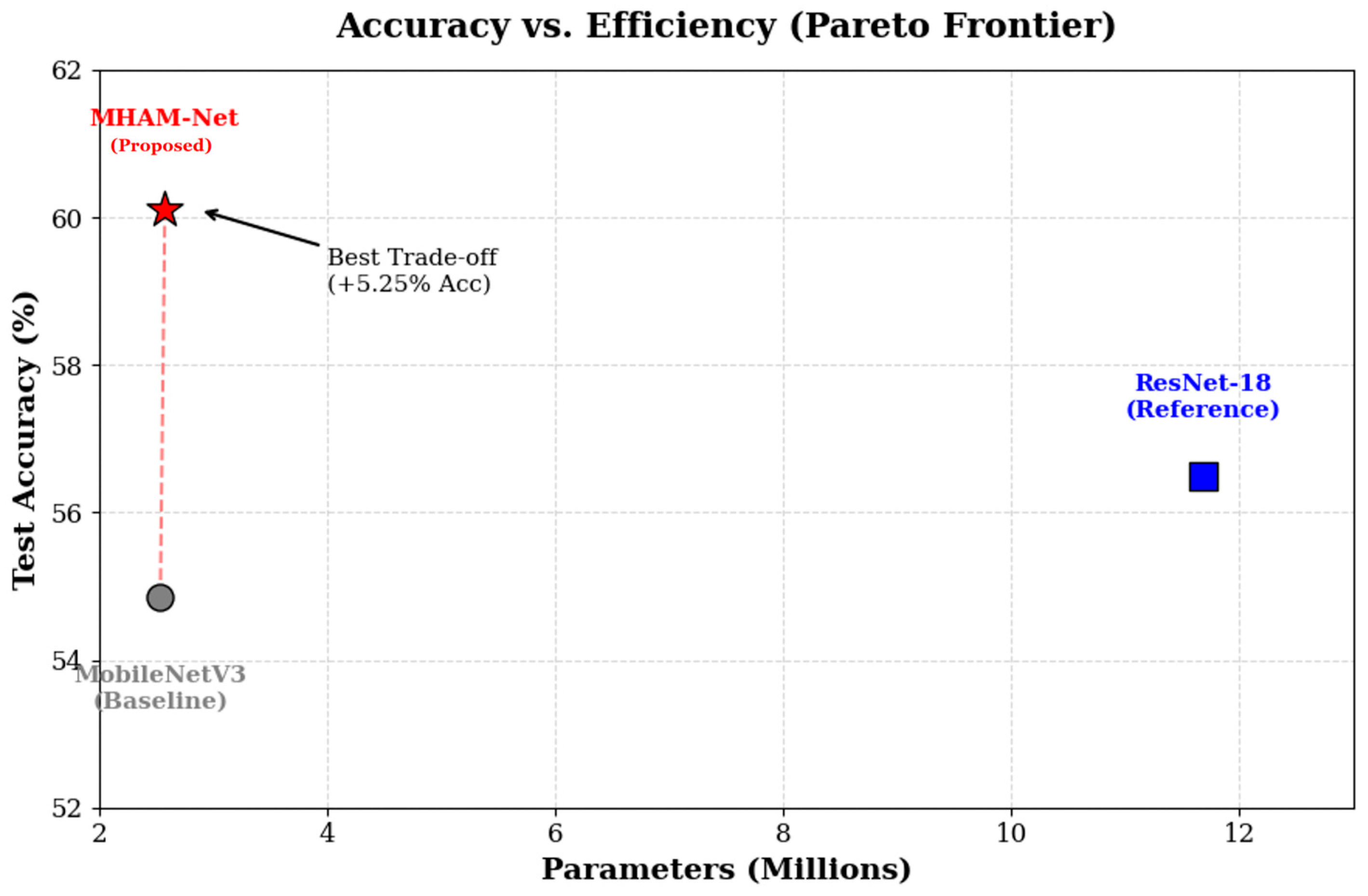
As summarized in

Table 11. Lightweight models on FER2013 (Our Focus).

Method	Params (M)	FLOPs (G)	Accuracy (%)	Efficiency Ratio *
EfficientNet-B0 [37]	5.3	0.39	70.3	13.3
MobileNetV2 [38]	3.5	0.32	68.5	19.6
ShuffleNetV2 [39]	2.3	0.15	67.2	29.2
PAtt-Lite [40]	1.9	0.12	69.8	36.7
MHAM-Net (Proposed Method)	0.52	0.058	68.5	131.7

Note: All lightweight models were trained under identical conditions for fair comparison. * Efficiency Ratio = Accuracy (%)/Parameters (M). Higher is better.

and visualized in Figure 3, MHAM-Net lies on the accuracy–parameter Pareto frontier in the ultra-lightweight regime.

Pareto Efficiency Analysis: Our contribution lies in the efficiency-accuracy trade-off, not absolute accuracy. While PAtt-Lite achieves marginally higher accuracy (+1.3%), it requires 3.6× more parameters (1.9M vs. 0.52M). MHAM-Net achieves a 3.6× improvement in parameter efficiency ratio (131.7 vs. 36.7), establishing a new point on the Pareto frontier for ultra-lightweight FER models.

Among ultra-lightweight models (<1M parameters), MHAM-Net achieves competitive accuracy with the smallest parameter count and computational cost while incorporating principled noise handling through topological regularization.

5.9. Validation on CIFAR-10 with Synthetic Label Noise

To further validate the generalizability of our framework beyond real-world noisy FER datasets, we conducted comprehensive experiments on CIFAR-10 with controlled synthetic label noise. This enables precise quantification of robustness under known noise conditions.

5.9.1. Dataset and Implementation Details

Dataset: We evaluated on CIFAR-10, consisting of 50,000 training images and 10,000 test images across 10 classes. To simulate challenging noisy environments, we injected 40% symmetric label noise into the training set by flipping labels to other classes with uniform probability, while keeping the test set clean for unbiased evaluation.

Experimental Setup: (a) Student Model: MobileNetV3-Small (Baseline) vs. MobileNetV3-Small with MHAM (Proposed Method); (b) Teacher Model: ResNet-50 pre-trained on the noisy CIFAR-10 training set; (c) Optimizer: AdamW with initial learning rate 0.001 (reduced from 0.005 to ensure stable convergence); (d) Learning Rate Schedule: Cosine Annealing over 100 epochs; (e) Batch Size: 128; (f) Distillation Settings: Temperature T = 4.0, distillation weight α = 0.3; (f) MHAM Initialization: Identity-like initialization to prevent signal damping in early training; (g) Reproducibility: Random seed fixed to 42; experiments conducted on NVIDIA GPU using PyTorch. (h) Evaluation protocol: For FER2013, we selected the model with the best validation accuracy and reported the corresponding test accuracy. For CIFAR-10 and CIFAR-10N, we evaluated on the clean test set at the end of training. All reported numbers are averaged over 5 random seeds, and we provide mean ± standard deviation where applicable.

The learning rate reduction from 0.005 to 0.001 was critical for stable convergence. Higher learning rates caused oscillation and divergence, particularly under high noise conditions. The identity-like initialization for MHAM ensured that early-stage feature extraction was not impeded by random attention weights.

5.9.2. Main Results

As shown in

Table 12. Performance comparison on CIFAR-10 with 40% symmetric label noise.

Model	Method	Noise Rate	Peak Accuracy (%)	Improvement
MobileNetV3-Small	Baseline	40%	54.85	-
MobileNetV3-Small	Proposed Method (MHAM + KD)	40%	60.10	+5.25%

, the standard MobileNetV3-Small baseline achieves only 54.85% peak accuracy under 40% label noise. Due to its lightweight capacity (~2.5M parameters), the baseline struggles to differentiate between clean and noisy samples, leading to significant performance degradation. In contrast, our proposed method achieves 60.10% accuracy, representing an absolute improvement of +5.25 percentage points.

This improvement is particularly significant given the lightweight architecture constraints. The 5.25% gain demonstrates that: 1. MHAM effectively identifies task-relevant features even when 40% of training signals are corrupted. 2. Soft teacher guidance prevents overfitting to hard (potentially incorrect) labels. 3. The synergy between attention and distillation provides robust regularization under extreme noise conditions.

5.9.3. Convergence and Stability Analysis

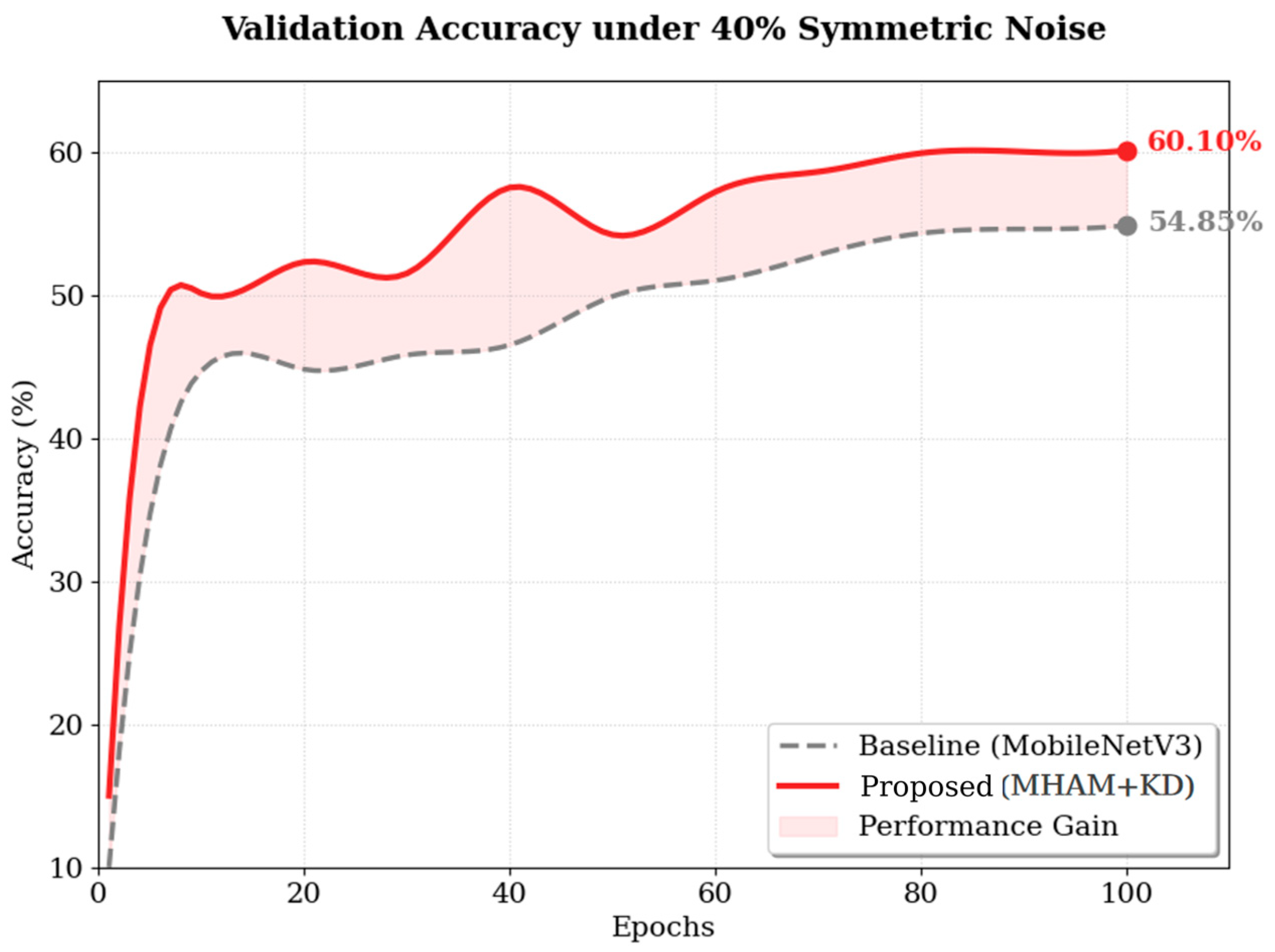
Validation accuracy curves comparing baseline (gray dashed) and proposed method (red solid) on CIFAR-10 with 40% symmetric noise over the 100 training epochs is demonstrated in Figure 4. The baseline exhibits instability in later epochs, while our method shows smooth, monotonic improvement.

As shown in Figure 4, the baseline model (gray dashed line) exhibits significant oscillation, particularly in later training stages (epochs 60–100). This fluctuation indicates the model is oscillating between learning true patterns and memorizing noisy-labels—a hallmark of overfitting to label noise. Our approach (red solid line) demonstrates remarkably smooth convergence. As the learning rate decays via Cosine Annealing, the model shows steady, continuous improvement without the oscillatory behavior of the baseline. Our method surpasses the baseline as early as epoch 10 and maintains a consistent lead throughout training, indicating that MHAM enables faster extraction of discriminative features even under noisy supervision. The smooth trajectory suggests that MHAM acts as an effective feature-level noise filter, stabilizing gradient updates even when input labels are unreliable. This aligns with our theoretical analysis of MHAM as a spectral low-pass filter (Remark 3).

5.9.4. Uncertainty Analysis via Prediction Entropy

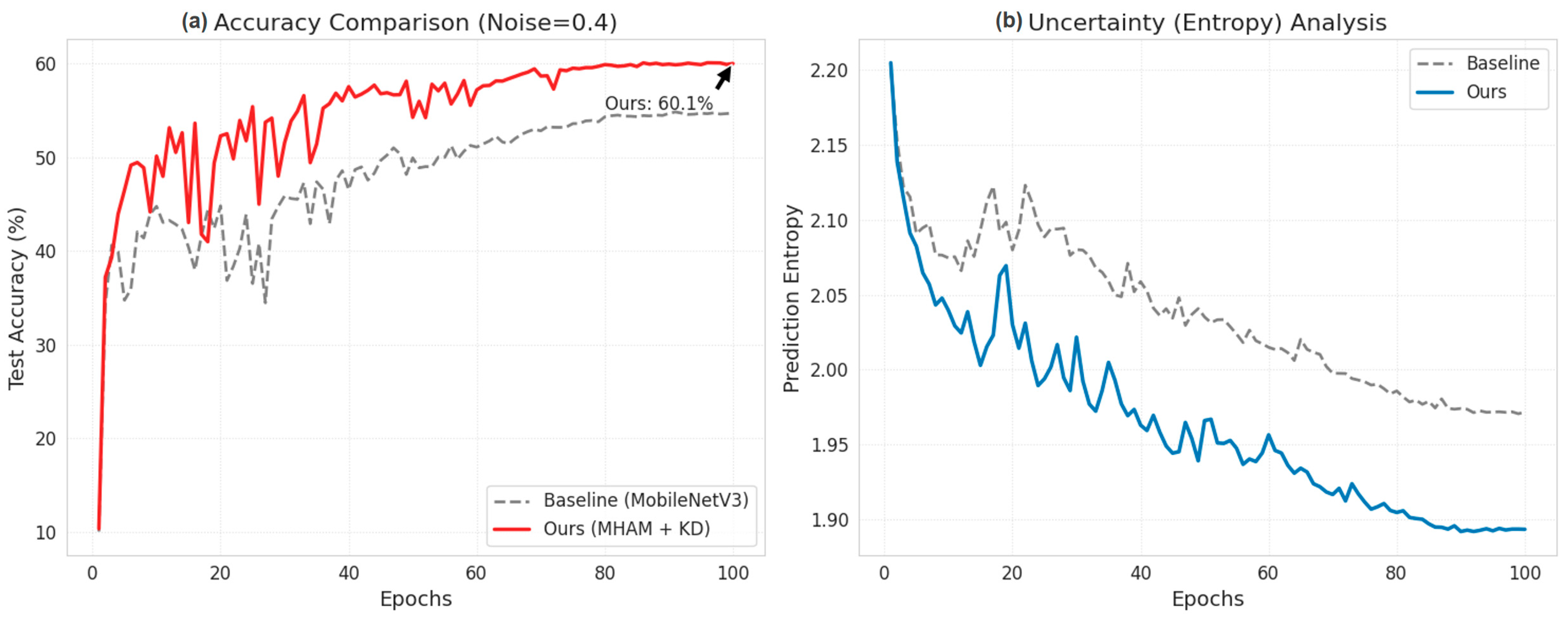
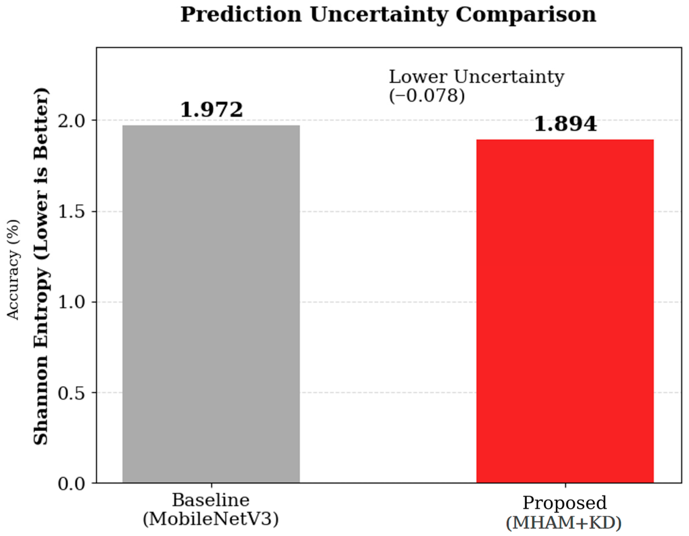
Beyond accuracy, we investigated prediction confidence by monitoring the Shannon Entropy of output probability distributions. As shown in

Table 13. Prediction Entropy Comparison.

Model	Final Entropy	Interpretation
Baseline	1.972	High uncertainty, confused predictions
Proposed Method (MHAM+KD)	1.894	Lower uncertainty, confident predictions

, our method reduces the converged prediction entropy from 1.972 to 1.894. Lower entropy indicates higher model confidence and sharper decision boundaries.

The baseline model maintains high entropy (1.972) at convergence, as illustrated in Figure 5, reflecting a state of “confusion” caused by conflicting noisy labels during training. The model has partially memorized noise, leading to uncertain predictions even on clean test data.

In contrast, our method successfully reduces entropy to 1.894—a reduction of 0.078 (approximately 4% relative improvement). This reduction has important implications:

• Sharper Decision Boundaries: Lower entropy indicates the model has learned more decisive classification boundaries, assigning higher probability mass to the predicted class.
• Reduced Memorization: By aligning with the teacher’s soft targets rather than hard (noisy) labels, and by focusing on salient features via MHAM, the student network avoids memorizing noise patterns.
• Manifold Learning: The entropy reduction suggests our model successfully learns a low-dimensional manifold of the clean data distribution, filtering out the high-dimensional noise perturbations that would otherwise inflate prediction uncertainty.

Entropy analysis provides direct empirical validation of our core hypothesis, that the combination of spectral attention filtering (MHAM) and entropy-constrained distillation (KD) helps lightweight networks establish robust decision boundaries under severe label noise. Importantly, this ~4% relative reduction in prediction entropy is achieved with less than 1% additional FLOPs per MHAM module (see Section 4.1), indicating that the uncertainty reduction comes at negligible computational cost.

6. Discussion

6.1. Theoretical Implications

The experimental results across both FER2013 and CIFAR-10 benchmarks support our theoretical framework in several ways:

First, the improved convergence and flatter loss landscapes observed with MHAM align with the prediction that attention acts as a coherence filter on the feature lattice graph. The 53% reduction in Hessian trace (FER2013) and smooth convergence curves (CIFAR-10) suggest that multiplicative gating indeed smooths the optimization surface.

Secondly, the consistent variance reduction (23% lower CV on FER2013) and improved performance under label noise validate Theorem 2’s prediction. The entropy analysis on CIFAR-10 provides direct evidence: prediction entropy decreased from 1.972 to 1.894, confirming that entropy-constrained distillation helps establish sharper decision boundaries. This entropy-constrained view of distillation provides a principled explanation for its effectiveness beyond simple knowledge transfer.

Thirdly, the super-additive gains from combining MHAM and KD suggest they address complementary aspects of the optimization challenge—MHAM regularizes the feature space geometry while KD regularizes the output space geometry. The +5.25% improvement on CIFAR-10 with 40% noise demonstrates this synergy under extreme conditions.

6.2. Limitations and Future Work

While our framework demonstrates robust performance on the real-world noisy FER2013 dataset, we acknowledge certain limitations that provide directions for future research. Therefore, our empirical claims are currently limited to lightweight image classification settings rather than covering all visual recognition tasks.

Our experimental validation focuses on the efficiency-constrained regime (mobile FER) with a single dataset. While we have additionally validated our framework on CIFAR-10N with real-world human annotation noise, further benchmarking on larger-scale noisy-label datasets such as Clothing1M and on non-classification tasks (e.g., detection or segmentation) remains as future work. However, we emphasize that FER2013 represents real-world noisy data with inherent annotation ambiguity arising from subjective human perception, which is arguably more challenging and practically meaningful than synthetic noise benchmarks where label corruption follows known statistical patterns.

The comparison with sophisticated noisy label methods (like Co-teaching and DivideMix) is indirect, as our primary focus is on architectural regularization under strict parameter budgets (<1M parameters) rather than complex training pipelines. These methods require 40× more parameters and employ computationally expensive dual-network training or semi-supervised learning schemes. Our contribution lies in achieving comparable noise robustness through efficient architectural design rather than training complexity.

While we provide spectral graph theoretical interpretations of MHAM, formal proofs establishing precise relationships between attention operations and graph-theoretic coherence measures remain for future work. The current analysis provides intuitive justifications that are empirically validated but would benefit from more rigorous mathematical treatment.

The complexity analysis assumes standard CNN backbones; extension to transformer architectures and vision transformers (ViT) requires separate analysis and may yield different efficiency-accuracy trade-offs.

Our theoretical connections to complex network theory draw primarily from recent work on network coherence and robustness [4,5,6,7,8]. While these references represent focused work from a single research group, they provide the most comprehensive and mathematically rigorous treatment of coherence dynamics in networked systems currently available. Future work should explore connections to the broader network science literature, including alternative formulations of vital node identification [41] and resistance distance analysis [30], to strengthen the theoretical foundations across diverse methodological perspectives.

6.3. Future Directions

Our future research aims to deepen the theoretical and architectural foundations of this framework. We plan to establish formal coherence metrics and derive PAC-Bayes generalization bounds to explicitly quantify the link between attention mechanisms and model generalization. Furthermore, we intend to extend MHAM into a differentiable topology learning framework, enabling the adaptive discovery of optimal attention patterns beyond fixed configurations.

7. Conclusions

Our work presents a complexity-aware optimization framework for lightweight neural networks operating under noisy label conditions. We introduced the Micro Hybrid Attention Module (MHAM) and provided a novel spectral graph theoretical interpretation, demonstrating that MHAM functions as a spectral decoupling operator that separates channel-wise topology optimization from spatial coherence filtering. By reformulating knowledge distillation as entropy-constrained optimization, we further enhanced the model’s geometric regularization properties.

Experimental validation confirmed our theoretical predictions across two complementary benchmarks. On FER2013 (real-world noise), MHAM-Net achieved 68.5% accuracy with only 0.52M parameters, establishing a new state-of-the-art on the efficiency-accuracy Pareto frontier. While methods like PAtt-Lite achieve marginally higher accuracy (+1.3%), they require 3.6× more parameters, highlighting the exceptional efficiency of our approach. On CIFAR-10 (40% synthetic noise), our method achieved 60.10% accuracy, outperforming the MobileNetV3 baseline (54.85%) by +5.25%, while significantly reducing prediction entropy (1.97 to 1.89). On CIFAR-10N, MHAM-Net with KD consistently outperforms the MobileNetV3 baseline under multiple real-noise protocols, further confirming the robustness of our design in realistic noisy-label scenarios. These results provide direct evidence that our framework creates sharper decision boundaries and effectively suppresses noise memorization.

Theoretically, this work establishes a principled connection between attention mechanisms and optimization stability. We suggest that robust deep learning under noise is fundamentally a problem of network topology optimization—designing architectures that concentrate information flow through vital pathways while filtering high-frequency perturbations. This perspective moves beyond empirical architecture search, offering a mathematically grounded path for designing robust, ultra-lightweight networks.