3. Minimal Patterns and Pattern Priority
In this section, we introduce the notions of minimality and pattern priority. The former will be used to avoid useless characters in the definition of a pattern, the latter as a means for comparison.
Definition 4 (Minimal representation ) Given a sequence, p, of length, k, the minimal representation of p is a sequence, , of length, k, with symbols, , for .
Remark 1 The minimal representation of a sequence is unique.
Remark 2 Since is more specific than p, that is, cannot have more occurrences in s than p, then the list of occurrences of must be the same as p.
Let be the minimal representation of a pattern, m, with sequence, p, then Remark 2 suggests to us that agrees with the definition of pattern (that is, is complete):
Definition 5 (Minimal pattern) The minimal representation of m, given by , is called a minimal pattern.
Computing the minimal representation of a pattern is useful when a pattern is composed by character classes. To have a more concrete idea about this concept,
Table 3 shows an example of minimal representation of the pattern
, where the reference string is
and the classes are
and
. In this case, we say that
is a minimal pattern. In practice, most of the functional patterns reported by PROSITE are not minimal.
Table 3.
Example of minimal representation of a pattern, m, with sequence, p.
Table 3.
Example of minimal representation of a pattern, m, with sequence, p.
| j | 1 | 2 | 3 |
|---|
| | | |
| a | | |
Let be a set of patterns with character classes lying on the string, s. From Remark 1 we have that each pattern, , has a unique minimal representation, . Thus, one can easily check that is an equivalence relation. Let us map all the patterns in into the set of their minimal version, , where each pattern, , is the minimal, , of some pattern, . Then, the set of patterns, , is partitioned into equivalence classes by the binary relation of equality between minimal patterns.
Remark 3 Two patterns, m and , in may have the same location list; thus, they will be mapped into the same minimal pattern, . On the other hand, two minimal patterns with the same location list must have different lengths.
We call the minimal set of . Since mapping in could mean a drastic reduction in the number of patterns, this is, in practice, a first step in filtering. Now, we define a simple property of patterns with character classes, the degeneracy, that is, the number of characters in a pattern.
Definition 6 (Degeneracy of a sequence ) The degeneracy of a sequence, p, of length, k, is defined as . The degeneracy of a pattern, , denoted by , is defined as the degeneracy of its sequence, .
For instance, given two sequences, and , their degeneracy is and . Therefore, the degeneracy of the pattern, , is equal to , that is, 6.
With this notion, we can define the priority between patterns, as a means for comparing different patterns. Note that several notions of priority can be established at this stage. We choose a very intuitive combination of pattern length, pattern degeneracy and location list.
Definition 7 (Pattern priority ‘→’) A pattern, m, of length, k, has priority over another pattern, , of length, , denoted, , if (1) , or (2) and , or (3) , , , when both minima exist.
For instance, consider , and . Then, m has priority over , written , because they have the same length and degeneracy, but . If two patterns, m and , have the same length and degeneracy, but either or , then we consider them incomparable; otherwise, they are comparable. Nevertheless, we will solve the non-comparability of two patterns with Theorem 2.
Given our binary relation, called pattern priority, we want to prove that some basic properties holds:
Definition 8 (Sub-ordered, totally ordered) Given a set, , if a binary relation, R, over this set is (i) irreflexive; m R never holds (ii) antisymmetric, ⇒ not R and R ; and (iii) acyclic, then is said to be sub-ordered. If R is also total, that is R or R , then is said to be totally sub-ordered. Furthermore, is said to be totally ordered if R is irreflexive, antisymmetric, transitive, that is R and R ⇒ m R and total.
Lemma 1 A set, , is totally ordered under a binary relation, R, if and only if it is totally sub-ordered.
Proof It is straightforward that transitivity implies acyclicity, that is, if is totally ordered, then is also totally sub-ordered. It is also easy to see that acyclicity and totality, together, imply transitivity. Consider a chain of patterns in : R , R , R . Since for acyclicity, R does not hold, then, for totality, R . Hence, transitivity holds and, therefore, the definitions totally sub-ordered and totally ordered coincide. ☁
Now, before showing that some of these properties hold, we need to prove two preliminary results for the pattern priority rule. At first, we observe the following.
Fact 1 The binary relation of pattern priority is irreflexive and antisymmetric (since properties (1), (2) and (3) of Definition 7 are strictly defined).
Lemma 2 Let m and be two patterns with , such that the two minima both exist, and define j to be . Then, the occurrences of m and at positions less than j must be the same.
Proof We have to prove that, in case (3) of Definition 7, the occurrences of m and less than j are identical. If m has an occurrence less than j that is not in , then , which is impossible by hypothesis. Conversely, if has occurrences less than j that are not in , then contradicts again our assumptions. Thus, the occurrences of the two patterns less than j must be the same, and we call them paired. Finally, by assumptions, it trivially holds that . ☐
Lemma 3 Let , , be a chain of patterns with the same length and degeneracy. Then, either or holds.
Proof We will prove the statement by induction on t. Let the basis be . In this case, the chain, , coincides with the result. We will show now that, if it holds either or , then either or holds.
Assume . Define j to be , this minimum exists, since (by property (3) of Definition 7). It follows that and, from Lemma 2, that the occurrences of and that are less than j are paired. Hence, these occurrences are shared also with . Since , then either holds (because j makes the difference between and ) or and are incomparable. In the latter case, and imply , which is impossible, since and are comparable by hypothesis. Thus, in this latter case, we have that .
Conversely, assume . Define j as before and . It holds that (as already observed), and that , because of . Then, by Lemma 2, the occurrences of and that are less than j are paired, and the same is true for the occurrences of and that are less than . It follows that, if and are comparable, there exists an occurrence in that is more on the left with respect to those of : If , the occurrences of , and less than are paired together, and thus, makes the difference; otherwise (), the occurrences of , and less than j are paired together, and hence, makes the difference. Alternatively, implies that the occurrences of equal to or less than are shared with , which leads to , which is impossible. ☁
Theorem 1 Any set of patterns, , is sub-ordered with respect to the binary relation of pattern priority.
Proof We have to prove that the relation of pattern priority is irreflexive, antisymmetric and acyclic. The first two properties are stated in Fact 1. Now, following the work in Lemma 3, we can prove that the acyclicity holds too. First, observe that length and degeneracy are intrinsic properties of the single pattern. If all patterns in have different lengths and degeneracies, then by definition of pattern priority, it is always true that either or , and a cycle can never exist, because of different lengths or degeneracies. Alternatively, consider a chain of patterns, , , with the same length and degeneracy. In this case, we must use property (3) of Definition 7 to compare the patterns together. From Lemma 3, it follows that a cycle of pattern priority between any chain of patterns is, again, impossible, and hence, the acyclicity holds. ☐
Note that the non-decision on some binary comparisons finally discards the relation of totality and, as seen above, of transitivity. For instance, consider and the patterns and with the same list of occurrences: In short, , and . This means that we are not able to compare m and using the pattern priority rule. Another example is given by , and . In this case, and , but does not hold, since . The issue is that these patterns are not minimal, like most of the patterns in PROSITE. In the following, we set the basis to solve this problem.
Theorem 2 Given any set of patterns, , its minimal set, , is totally ordered under the binary relation of pattern priority.
Proof Along with Theorem 1, we have that any set of patterns, , is sub-ordered under pattern priority; thus, also the set of minimal patterns, , is sub-ordered. Following Lemma 1, we have to prove that the totality holds on this new set, , that is, every pair of minimal patterns must be comparable under pattern priority. In other words, if , it must hold either or .
From Remark 3, we have that for two minimal patterns, m and , with the same length, and thus, we have, without loss of generality, two cases to consider: or . From now, m and will be two minimal patterns with the same length and, for the former case, also with the same degeneracy . Thus, in the former case, if we consider and , the two minima exist and are different from each other; hence, it holds that either or , respectively, if the minimum of the two sets is either in or in . In the latter case, , since m and are minimal patterns, and the respective location lists are complete (that is, the respective patterns of m and must be different); therefore, it holds that . Thus, for any set of minimal patterns under pattern priority, the totality holds. From Lemma 1, we can conclude that any set of minimal patterns is totally ordered under the pattern priority rule. ☐
As a consequence of Theorem 2, all minimal patterns can be compared and ranked. We can further observe that every minimal pattern has priority over the patterns within its equivalence class, due to property (2) of pattern priority. Now, it is clear that any set of patterns can be mapped into its minimal representative set and that we can build a measure of total order over this set.
5. Experimental Results
In this section, we discuss the ability of underlying patterns to efficiently capture meaningful biological information. A general problem in genome and proteome research is the identification of signals represented by means of degenerate patterns. In this sense, some modern degenerate pattern discovery tools proved to be useful in biological sequence analysis, as we have discussed at the beginning of the paper. Here, we first collect the degenerate patterns in the output from one of these tools, say a set of patterns, , and then, present some preliminary experimental results in order to support the theoretical properties shown in the above sections.
More generally, there are two types of scenarios where the notion of underlying patterns could be useful. The first case is when a region of interest has already been identified, so that it is possible to analyze and select only those patterns that are underlying with respect to that particular region, without considering the whole set of patterns. Another possible application is the case where we just want to filter all patterns in , looking at the whole sequence.
In this context, we present some results for the latter scenario. We take as input,
, the set of patterns extracted by Varun [
12,
25], a tool for
de novo pattern discovery. The dataset consists of six protein families for which Varun successfully extracts the representative patterns contained in the PROSITE signatures (release 20.85) [
12]. For each signature, we select all sequences in the Swiss-Prot database that share that signature. In summary, our dataset is the following.
Nickel-Dependent hydrogenases (id PS00508; in short, Ni). These are enzymes that catalyze the reversible activation of hydrogen and are further involved in the binding of nickel. The family is composed by 22 sequences of about 12,300 amino acids in total. This family contains two representative signatures, RG[FILMV]E...............[EM PQS][KR].C[GR][ILMV]C and [FY]D[IP][CU][AILMV][AGS]C.
Coagulation factors 5/8 type C domain (FA58C) (id PS01286; in short, Fa). This family is composed by 40 sequences of about 46,500 amino acids in total. They share two signatures: [FWY][ILV].[AFILV][DEGNST]......[FILV]..[IV].[ILTV][KMQT]G and [LM]R.[EG][ILPV].GC.
Formate and nitrite transporters (id PS01005; in short, Form). The signature [LIVMA][LIVMY].G[GSTA][DES]L[FI][TN][GS] is present in 17 sequences of a total length of 5300 amino acids.
Ubiquitin-Activating enzyme (id PS00865; in short, Ubi). The active site P[LIVMG]CT[LIVM][KRHA].[FTNM]P appears in 36 proteins of about 25,200 amino acids in total.
RNA polymerases M/15 Kd subunits (id PS01030; in short, Poly). The representative signature [FY]C.[DEKSTG]C[GNK][DNSA][LIVMHG][LIVM] occurs in 29 sequences of about 4000 amino acids.
Dbl homology domain (id PS00741; in short, Dbl). The signature [LM]..[LIVMFYWGS][LI]..[PEQ][LIVMRF]..[LIVM].[KRS].[LT].[LIVM].[DEQN][LIVM]... [STM] appears in 65 sequences of a total length of 18,750 amino acids.
To prove that the information captured by the underlying patterns is relevant with respect to the protein families under examination, we devised two kinds of tests. In the first test, we compare the original set of patterns in the input, , with the set of underlying patterns in the output, , using global measures. In the second, we investigate the ability to filter a list of meaningful patterns and retain the representative ones, perhaps with a higher rank.
In the first set of experiments, we use Varun to extract patterns from the above families of protein sequences for different quorums,
q. For each family, we concatenate the sequences and extract patterns from the concatenation; thus, in all the experiments, the quorum refers to the number of occurrences in the concatenation of all sequences of a certain family. This notion of quorum can generate several spurious patterns and, thus, will make the filtering problem more challenging. We also investigate a different setup in which the quorum value reflects the number of sequences where the pattern is contained. This latter scenario produces similar results; however, the range of values for this quorum is bounded by the number of sequences, and this can limit the possibility to study the efficiency of the filtering process, while varying the quorum values. For these reasons, we choose to use the first definition of quorum. Then, we use the extracted patterns as input to our algorithm, presented in
Section 4, in order to compute the underlying patterns
. In our experiments, each pattern,
, extracted by Varun is with character classes and no gaps, where we set the quorum,
q, for the underlying patterns, to be the same as the quorum for the original patterns in the input, as by the definition seen above. The length,
n, of the string in the input is equal to the length of the concatenations reported above. The size of
varies with respect to the quorum,
q, and for some configurations, can be larger than the sequence length (see
Figure 1). All experiments were conducted on a common PC, and the filtering process requires on average less than 10 s.
Figure 1.
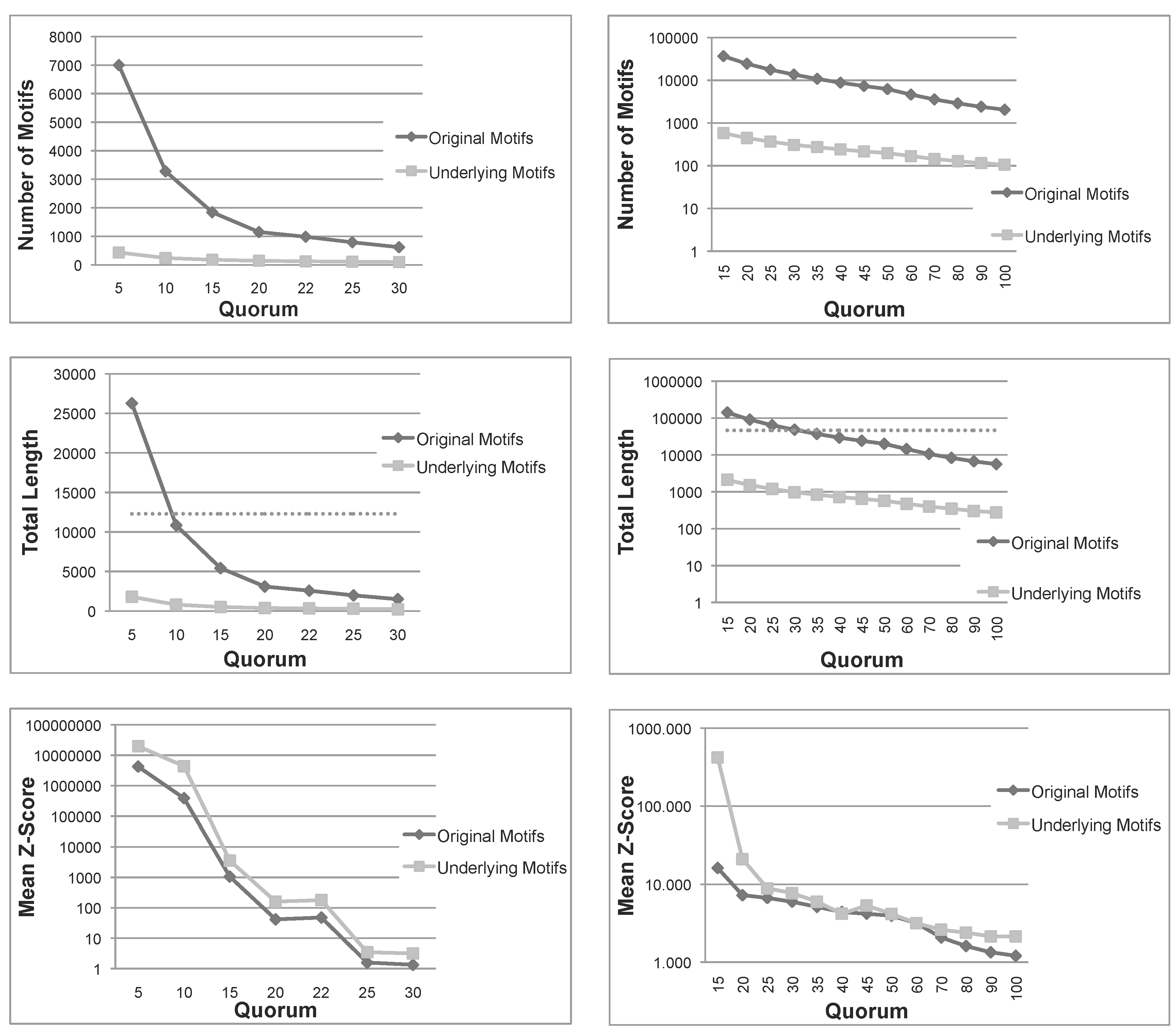
Total number, sum of lengths and mean z-score of the patterns extracted using Varun and their corresponding underlying patterns, for the two protein families, and . The dashed line in the total length diagrams indicates the total size of each family. Note that in (a) Mean Z-Score and (b) All diagrams, the ordinate is plotted on a logarithmic scale. (a) Nickel-Dependent hydrogenases (); (b) Coagulation factors 5/8 type C domain ().
Figure 1.
Total number, sum of lengths and mean z-score of the patterns extracted using Varun and their corresponding underlying patterns, for the two protein families, and . The dashed line in the total length diagrams indicates the total size of each family. Note that in (a) Mean Z-Score and (b) All diagrams, the ordinate is plotted on a logarithmic scale. (a) Nickel-Dependent hydrogenases (); (b) Coagulation factors 5/8 type C domain ().
For both sets of patterns,
and
, we compute some global statistics.
Figure 1 shows the number of patterns, the sum of lengths of all patterns and their mean
z-score for the first two protein families (
,
). The other families share the same behavior (figure not shown). The
z-score is computed employing the same formula reported in [
12]. As expected, the number of underlying patterns is always much smaller than the number of the original patterns. A similar conclusion can be drawn for the sum of lengths. More importantly, for small quorums, the total length of original patterns exceeds the length of sequences in both families, indicating that the original patterns are even larger than the set of sequences under examination. Moreover, as seen above, the sum of lengths of underlying patterns is always bounded by the length of sequences. These first two measures indicate that, not only the number, but also the total length of underlying patterns are much smaller than those of the original patterns. Therefore, the filtering process is space-efficient, as expected.
Another important measure is the mean
z-score of
and
. The
z-score of a pattern,
p, is a statistical measurement of the degree of over-representation of
p with respect to the expected number of its occurrences. The mean
z-score is thus a global measure able to capture the average quality of patterns in a set; however, it is much more computationally expensive than our pattern priority, and we just use it to validate our approach. In
Figure 1, we can see that, for all quorums, the average
z-score of underlying patterns is always greater than those of original patterns, and in most cases, the difference is one or two orders of magnitude. To summarize, this first test confirms that the number and span of underlying patterns is much more manageable than the original set and, also, that their average quality is improved.
Once we have verified that the notion of underlying is a suitable filter, in a second series of experiments, we test the ability to retain meaningful patterns. To this end, we employ the candidate patterns obtained from the previous experiments to test the presence of PROSITE signatures. We consider in detail again the first two families,
and
, and the corresponding signatures. The other four families show similar results and are summarized in
Table 4.
We consider
and
directly as degenerate patterns, due to their low number of gaps, while we split signatures,
and
, into two different patterns each and compute the statistics of these patterns accordingly. For both sets of patterns,
and
, we compute the maximum similarity between each pattern in the set and the two signatures. The similarity between two patterns,
m and
, is the number of shared characters, including character classes, in the best alignment of
m versus , without considering indels.
Table 5 and
Table 6 summarize the maximum similarity, for different quorums, of
and
, with each signature of the two protein families,
and
. The second and third columns report the maximum similarity for the set of underlying patterns divided by the similarity of the original set. For example, in the first row of
Table 5, the quorum is five. In this case, the maximum similarity of
with the representative pattern,
, is 26. The same value is obtained also for the corresponding set of underlying patterns,
, thus indicating that the pattern,
, is retained with the same degree of accuracy.
Table 4.
Comparison of performance between different binary relations applied to the underlying patterns: Pattern priority, z-score, probability with distribution based on the amino acid frequencies in s, probability with no background (i.e., each amino acid scores ), frequency of patterns in s, inverse frequency and the lexicographic order of occurrences. For each family, we summed up the maximum similarity with the two representative patterns for all quorums. Similarly, in the column rank, we show the average rank of the closest candidates to these patterns.
| | | |
|---|
| Binary Relation | Similarity | Rank | Similarity | Rank |
|---|
| Pattern priority | 151/157 | 2.78 | 247/264 | 5.34 |
| z-Score | 127/157 | 5.00 | 223/264 | 9.96 |
| Probability | 127/157 | 5.00 | 223/264 | 9.96 |
| Equal Probability | 127/157 | 5.00 | 223/264 | 9.96 |
| Frequency | 93/157 | 22.78 | 168/264 | 9.42 |
| Inverted frequency | 118/157 | 6.14 | 212/264 | 5.69 |
| Lexicographic order | 93/157 | 5.50 | 142/264 | 11.77 |
| | Form | Ubi | Poly | Dbl |
|---|
| Binary Relation | Similarity | Rank | Similarity | Rank | Similarity | Rank | Similarity | Rank |
|---|
| Pattern priority | 186/205 | 4.72 | 190/198 | 3.40 | 215/234 | 4.25 | 498/522 | 5.20 |
| z-Score | 167/205 | 6.00 | 178/198 | 4.74 | 212/234 | 5.86 | 455/522 | 7.10 |
| Probability | 167/205 | 6.00 | 178/198 | 4.74 | 210/234 | 5.92 | 455/522 | 7.10 |
| Equal Probability | 165/205 | 6.20 | 178/198 | 4.74 | 210/234 | 5.92 | 452/522 | 7.10 |
| Frequency | 102/205 | 26.62 | 112/198 | 9.75 | 135/234 | 13.69 | 321/522 | 21.35 |
| Inverted frequency | 154/205 | 7.92 | 159/198 | 6.00 | 188/234 | 10.10 | 436/522 | 13.74 |
| Lexicographic order | 105/205 | 16.44 | 112/198 | 12.39 | 126/234 | 13.93 | 308/522 | 22.00 |
Table 5.
Normalized maximum similarity with the reference patterns of the family nickel-dependent hydrogenases, for different quorums.
Table 5.
Normalized maximum similarity with the reference patterns of the family nickel-dependent hydrogenases, for different quorums.
| Quorum | Max Similarity | Max Similarity |
|---|
| (underlying/original) | (underlying/original) |
|---|
| 5 | 26/26 | 9/12 |
| 10 | 18/18 | 12/12 |
| 15 | 11/11 | 9/12 |
| 20 | 9/9 | 12/12 |
| 22 | 9/9 | 12/12 |
| 25 | 6/6 | 6/6 |
| 30 | 6/6 | 6/6 |
Table 6.
Normalized maximum similarity with the reference patterns of the family coagulation factors 5/8 type C domain, for different quorums.
Table 6.
Normalized maximum similarity with the reference patterns of the family coagulation factors 5/8 type C domain, for different quorums.
| Quorum | Max Similarity | Max Similarity |
|---|
| (underlying/original) | (underlying/original) |
|---|
| 15 | 11/12 | 11/12 |
| 20 | 11/12 | 12/12 |
| 25 | 12/12 | 8/10 |
| 30 | 10/12 | 8/10 |
| 35 | 10/12 | 9/10 |
| 40 | 10/12 | 8/8 |
| 45 | 12/12 | 8/8 |
| 50 | 12/12 | 8/8 |
| 60 | 10/10 | 8/8 |
| 70 | 10/10 | 8/8 |
| 80 | 9/10 | 8/8 |
| 90 | 9/10 | 8/8 |
| 100 | 9/10 | 8/8 |
In principle, the binary relation of pattern priority can be replaced by any other traditional means of comparison. To this end, we compared the pattern priority rule with other standard ranking methods that were applied to the underlying filtering step.
Table 4 reports the average scores for each measure for all six protein families, where a large maximum similarity with the two PROSITE signatures and a higher rank are preferable. In this context, we consider different ranking methods: The lexicographic order of patterns (Lexicographic), the number of occurrences (Frequency) and its inverse (Inverted Frequency). Other statistical ranking methods are also considered here: Pattern probability assuming either an i.i.d. distribution of symbols based on amino acid frequencies (Probability) or an equal distribution of symbols (Equal Probability);
z-score, computed using the probability value as in [
12].
We can easily see that our pattern priority achieves the best scores among all methods for the detection of representative patterns. In addition, our heuristic ranks on average the reference patterns of
in the top three out of 2239 candidate patterns in the input and those of
in the top five out of 10,842 patterns, while for the other families, the reference patterns range from the top three to the top five selected patterns, on average. The definition of pattern priority was conceived especially for degenerate patterns, like those presented in this section. However, this framework can be used in conjunction with other comparison functions designed specifically for patterns with profiles or variable gaps, e.g., [
38].
These preliminary experiments support the validity of the theoretical results presented in the previous sections and also prove their effectiveness for protein analysis. However, a more comprehensive experimental setting is desirable, in order to improve the evidence on the performance and to compare this method with other existing tools, like MEME [
42].


