A Stable Gaussian Fitting Procedure for the Parameterization of Remote Sensed Thermal Images

Abstract

An image analysis procedure based on a two dimensional Gaussian fitting is presented and applied to satellite maps describing the surface urban heat island (SUHI). The application of this fitting technique allows us to parameterize the SUHI pattern in order to better understand its intensity trend and also to perform quantitative comparisons among different images in time and space. The proposed procedure is computationally rapid and stable, executing an initial guess parameter estimation by a multiple regression before the iterative nonlinear fitting. The Gaussian fit was applied to both low and high resolution images (1 km and 30 m pixel size) and the results of the SUHI parameterization shown. As expected, a reduction of the correlation coefficient between the map values and the Gaussian surface was observed for the image with the higher spatial resolution due to the greater variability of the SUHI values. Since the fitting procedure provides a smoothed Gaussian surface, it has better performance when applied to low resolution images, even if the reliability of the SUHI pattern representation can be preserved also for high resolution images.

1. Introduction

Since decades, with the advent of earth observation satellites, remote sensing technology has been widely utilized to produce images of the Earth surface with different spatial resolutions. Frequently the analysis of these maps with visual inspection or statistical tools is not enough for quantitative monitoring and comparisons, and different approaches are required.

Several remote sensing images of geophysical variables could be conveniently represented by a suited fitting surface, able to parameterize and quantify the spatial distribution of the mapped quantity. In particular, satellite images mapping the land surface temperature (LST) over urban areas or the associated urban heat island (UHI) could be successfully fitted by a two-dimensional (2D) Gaussian distribution [1]. The SUHI intensity describes the difference in temperature between the urban locations and the surrounding rural background, and the SUHI effects have been analyzed for several decades, starting from Oke studies [2,3]. The monitoring of spatial and temporal parameters related to SUHI maps may allow the detection of health risk areas [4] and suggests modifications to the urban planning in order reduce the heat effects [5].

If a SUHI image is centered over an urban area, where the LST is higher with respect to the adjacent rural area, the heat island pattern can be spatially described by a Gaussian surface. With a fast and robust implementation of the fitting technique, such images can be parameterized in order to better understand the intensity, shape and orientation of the SUHI and also to perform quantitative comparisons among different images in time and space [6].

Different fitting methods can be adopted to generate Gaussian surfaces [7]: in this work the proposed approach is computationally quick and effective, without the occurrence of instability or convergence failure, failure that sometimes other fitting methods could encounter [7]. This is achieved by means of an initial guess parameter estimation performed by a multiple linear regression image-based, before the iterative nonlinear fitting, ensuring stable results.

The Gaussian fit was executed in Matlab (The MathWorks, Release 2010a).

A detailed description of the different steps of the fitting procedure is provided, and the results of the parameterization and the algorithm performance are shown both for low-resolution and high resolution images. The processing of the SUHI maps computed from data of two satellite sensors of different spatial resolution (MODIS and Landsat Thematic Mapper, with 1 km and 30 m pixel size, respectively) will also point out the impact of the image detail definition on the fitting representation.

2. Gaussian Fitting

For SUHI or LST map analysis, a 2D Gaussian intensity distribution can be a reliable representation of the expected pattern, especially when an urban area shows an evident heat island with respect to the surrounding rural areas. This fitting procedure can also be suitable for the analysis of maps describing the spatial distribution of quantities having clustered high values tending to decrease branching off into the map perimeter.

For this purpose a fast and robust Gaussian fitting technique is implemented to analyze and parameterize the spatial distribution of the SUHI for a selected urban area. This technique also provides a tool to perform quantitative comparisons between different SUHI maps useful for inter-city comparisons or for single city analysis over different time scales. The enclosed plotting procedure allows a further better understanding of the shape and orientation of the heat island for each image.

Each SUHI map is processed using a method described by Streutker [1,8]. In this technique a Gaussian surface is used to fit the spatially distributed heat island signatures as follows:

$$SUHI\left(x,y\right)=a_0\times \text{exp}\left[-\frac{{\left(\left(x-x_0\right)cos\varphi +\left(y-y_0\right)sin\varphi \right)}^2}{0.5a_x^2}-\frac{{\left(\left(y-y_0\right)cos\varphi -\left(x-x_0\right)sin\varphi \right)}^2}{0.5a_y^2}\right]$$

(1)

where (x,y) represents the location of a pixel. Such a least-square fit provides not only an estimate of the magnitude (a₀) of the SUHI intensity for the selected area, but also of the spatial extent (a_x and a_y), orientation (φ), and the central location (x₀ and y₀) of the heat island.

The two spatial extent parameters can be combined to determine the overall area or footprint of the SUHI. The footprint has the form of an ellipse (horizontal cross-section of the Gaussian surface) with the major and minor axes equivalent to the a_x and a_y extent parameters, φ is the angle at which the major axis forms with the x-axis; the central location (x₀, y₀) is defined as the shift with respect to the center of the map.

The SUHI intensity within such an ellipse is maximum in the center (x₀, y₀): the distance from the center at which the temperature decreases up to a level of e^-1/2, or 61%, of its maximum value a₀, identifies a footprint that will be named A_61%. Also, can be useful to compute the area of the SUHI for which the temperature is greater than a constant threshold instead of a fraction of the maximum, for example greater than 1.0 K (A_1K).

This fitting method is not influenced by localized high surface temperatures within the image, smoothing isolated peaks as will be illustrated in the result section.

In the next section the main steps of the algorithm performing the Gaussian fit are described.

3. Algorithm Implementation

The fitting procedure was implemented in Matlab, and the structure can be divided in the following parts:

-

Input: matrix of gridded data to fit and correspondent spatial coordinates (latitude, longitude).

-

Initial guess parameter estimation: a multiple linear regression image-based, i.e., a least square fit, is performed. Considering eq.1, it is possible to exactly transform it to a linear equation through the use of the logarithm, which can equivalently be expressed as a linear equation with six unknowns:

$$\ln \left(SUHI\left(x,y\right)\right)=a_1{x}^2+a_{2}xy+a_3{y}^2+a_{4}x+a_{5}y+a_6$$

(2)

where the coefficients a_i are directly estimated by using a linear regression.

-

Gaussian fitting: starting from the initial guess parameters, a nonlinear data-fitting in least-squares sense is executed. It is an iterative fitting procedure implemented with the function lsqcurvefit.m (Matlab Optimization Toolbox), that finds the coefficients that best fit the Gaussian function to the data (the UHI image in this case) in the least-squares sense [9,10].

-

Output: from the fitting coefficients obtained from the previous step, the parameters a₀, a_x, a_y, φ, x₀, y₀ are directly computed on the basis of eq. 1 and eq. 2, together with A_61% and A_1K and the correlation coefficient between the Gaussian model and the SUHI image.

-

Graphical output: the results of the Gaussian fitting are illustrated visualizing the 2D SUHI map superimposing the oriented footprint of the SUHI fitting, i.e., the horizontal cross-section of the Gaussian surface. Also, a 1D plot of the SUHI map is produced considering a vertical cross-section of the Gaussian surface along the major and the minor axes.

4. Satellite Images Processed

The study area of the SUHI pattern is Milan, North Italy, with city center located at 45.47° N and 9.18° E. The summer is generally hot, with some urban areas affected by high temperatures and humidity [11]. In this study, data acquired by the MODIS instruments on the Terra and Aqua satellites were employed, passing over the Milan area four times a day. The LSTs extracted from the MOD11A1 and MYD11A1 products, with a 1-km spatial resolution and with an accuracy better than 1.0 K [12], were used to compute the SUHI of the city. Although the 1-km spatial resolution of MODIS may represent a limitation for a finer scale monitoring, the four daily passes of the sensor allow an investigation of the urban heat island at different temporal scales.

While low-resolution satellite data are adequate for studying the large-scale SUHI characteristics, it is useful for urban planners to use also high-resolution thermal data to monitor the heat island intensity on a smaller scale, with the aim to control or mitigate the effects of the SUHI in relation to population density and land cover.

For the high resolution image on the same area (pixel of 30 m), data provided by the Thematic Mapper (TM) instrument onboard Landsat-5 platforms were used. This satellite passes over the same area every 16 days, and therefore has a lower frequency of revisit time. The Landsat TM sensor is composed by seven bands, six of them in the visible and near infrared (TM1-5, TM7), and one band in the thermal infrared region (TM6). TM has a native spatial resolution of 30 m for the six reflective bands and 120 m for the thermal band. TM6 is also delivered at 30 m, resampled with a cubic convolution by the US Geological Survey (USGS) Center website [13]. TM data were processed according to the calibration technique proposed by Chander [14], applying an atmospheric correction using the Chavez COST method [15]. The land surface temperature was retrieved from the Landsat TM thermal channel by inversion of the radiative transfer equation applied to the thermal infrared region [16].

Then, SUHI intensity maps were produced from each LST image, computing the difference in temperature between the urban locations and the surrounding rural background. For this purpose, pixels ascribed to the urban area were temporarily masked out using the land cover map of the MODIS products, producing an image consisting entirely of rural pixels. Each rural temperature image was fit to a planar surface, and then subtracted from the LST image, obtaining the SUHI pattern.

5. Results

The produced SUHI maps were fitted to a Gaussian surface after masking out the cloudy pixels, and then the parameters describing the magnitude (a₀), the spatial extent (a_x, a_y), the orientation (φ) and central location (x₀, y₀) of the heat island pattern were computed. An area around the Milan city center of 39 km² was selected, comprising the outskirts, neighboring municipal districts, industrial estates and rural areas. The application of the algorithm to both MODIS and Landsat TM images was analyzed visualizing the 2D (maps with footprint) and the 1D (along the two footprint axes) fitting results.

First, two issues have to be pointed out in the performance assessment:

-

The initial guess parameter estimation performed by an image-based multiple linear regression was advantageous with respect to a priori fixed parameters. In fact the latter choice was implemented as a test with different initial parameter combinations and instable results for several images were found: for instance, the iterative optimization was found to occasionally fail to converge, returning infinite or undefined results. This never occurred with the regressed initial parameters. Also, another possible choice of fixing the initial parameters by means of visual inspection of each image is not a straightforward way, yielding to a not automatic tool.

-

Cmputational time: instantaneous for the MODIS image (39 × 39 pixels), few seconds for the Landsat TM image (1307 × 1307 pixels). These performances were obtained by using a 3 GHz CPU.

5.1. 2D Results

An example of SUHI Gaussian fit for the MODIS images of the August 19, 2009, considering the four daily passes of the satellite sensor, is shown in Figure 1, plotting the 39 km × 39 km area around the Milan city center. Hours are reported in Central European Summer Time (CEST) date format, where CEST=UTC + 2, i.e., the local time of the city. For each image, the descriptive parameters for the Gaussian fit of the SUHI(x,y) map are reported in Figure 1. The two spatial extent parameters a_x and a_y define the footprint of the SUHI pattern, with orientation φ and center x₀, y₀: the blue inner ellipse (horizontal cross-section of the Gaussian surface) superimposed on the maps corresponds to A_61%, while the black outer ellipse represents the area A_1K.

A correlation coefficient (corr, reported in Figure 1) was computed between the SUHI values of the image and the Gaussian surface used to fit the SUHI map.

The four daily passes of the MODIS sensor allow an investigation of the heat island trend during the whole diurnal cycle. The employment of the proposed Gaussian fitting points out quantitatively the magnitude, extent, shape and location of the SUHI pattern and detects the variations during the day. For instance, it is evident the greater footprints and magnitude for the daytime images with respect to the nighttime ones, and the change of orientation. A statistical analysis of MODIS images acquired during different years and fitted using this method is reported in [6].

Then, the SUHI map retrieved using the Landsat TM data acquired over Milan on August 6, 2009 at 12:00 CEST was processed, allowing to analyze the performance of the fitting procedure for a high resolution image on the same area (pixel 30 m). As in the previous figure, Figure 2 reports again the SUHI map with the Gaussian footprints and the correspondent descriptive parameters.

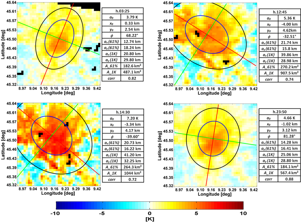
Figure 1. Surface urban heat island (SUHI) [K] over Milan (August 19, 2009) using MODIS data (39 × 39 pixels), with superimposed the horizontal cross-sections of the Gaussian surface. The descriptive parameters of the Gaussian fitting are also reported. Black pixels are cloudy pixels.

Figure 1. Surface urban heat island (SUHI) [K] over Milan (August 19, 2009) using MODIS data (39 × 39 pixels), with superimposed the horizontal cross-sections of the Gaussian surface. The descriptive parameters of the Gaussian fitting are also reported. Black pixels are cloudy pixels.

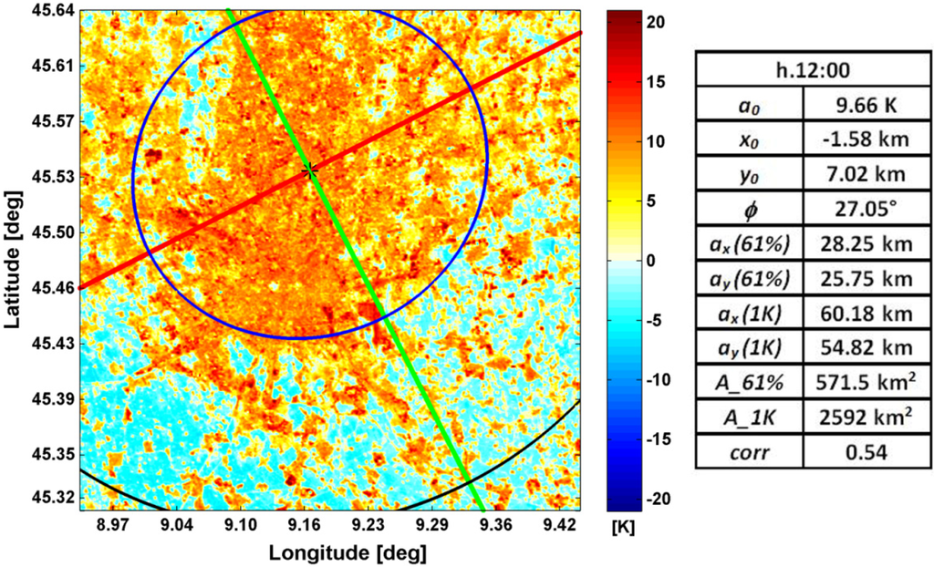
Figure 2. SUHI [K] over Milan (August 6, 2009) using Landsat TM data (1307 × 1307 pixels), with superimposed the horizontal cross-sections of the Gaussian surface. The descriptive parameters of the Gaussian fitting are also reported.

Figure 2. SUHI [K] over Milan (August 6, 2009) using Landsat TM data (1307 × 1307 pixels), with superimposed the horizontal cross-sections of the Gaussian surface. The descriptive parameters of the Gaussian fitting are also reported.

As expected, the impact of the higher spatial resolution on the fitting representation of the SUHI pattern shows some differences with respect to the lower resolution, such as the growth of the extent parameters and magnitude a₀, and therefore of A_61% and A_1K, and a reduction of the correlation coefficient. This is mainly due to the highest temperature values located in the urbanized areas that are preserved inside a pixel of 30 m, while they are smoothed in the averaging process inside a 1 km pixel. Also, clear differences emerge in the detail definition of the SUHI pattern between the two figures, pointing out the different ability to resolve sharp thermal discontinuities in a heterogeneous area. In particular, since the Gaussian fitting produces a smoothed surface, the higher variability of the pixel values for the Landsat TM image leads to a decrease of the correlation coefficient, even if the parameterization preserves the representativeness of the heat island pattern for the Milan area. It is worth to note how the different range of variation of the SUHI values, with higher values for the Landsat TM image, induces an increase of the spatial parameters with respect to the ones of the MODIS image. These aspects are confirmed in the next sub-section.

5.2. 1D Results

The results of the MODIS and Landsat TM image fitting are shown in the next figures visualizing the 1D plot obtained with a vertical cross-section of the Gaussian surface along the two footprint axes. The parameter values are the ones reported in Figure 1 and Figure 2.

Figure 3 and Figure 4 confirm how the MODIS image, where inside the pixels of 1 km the thermal discontinuities and the temperature peaks are averaged, is well correlated with the Gaussian surface, especially during the nighttime. The same 1D results for the Landsat TM image is shown in Figure 5.

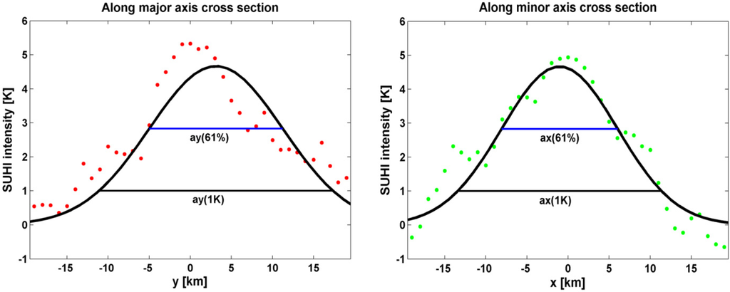
Figure 3. MODIS, August 19, 2009, 23:50. SUHI [K] correspondent to the vertical cross-section of the Gaussian surface along the major axis (left panel) and along the minor axis (right panel). The axes a_x and a_y for the two ellipses of area A_61% and A_1K are also reported.

Figure 3. MODIS, August 19, 2009, 23:50. SUHI [K] correspondent to the vertical cross-section of the Gaussian surface along the major axis (left panel) and along the minor axis (right panel). The axes a_x and a_y for the two ellipses of area A_61% and A_1K are also reported.

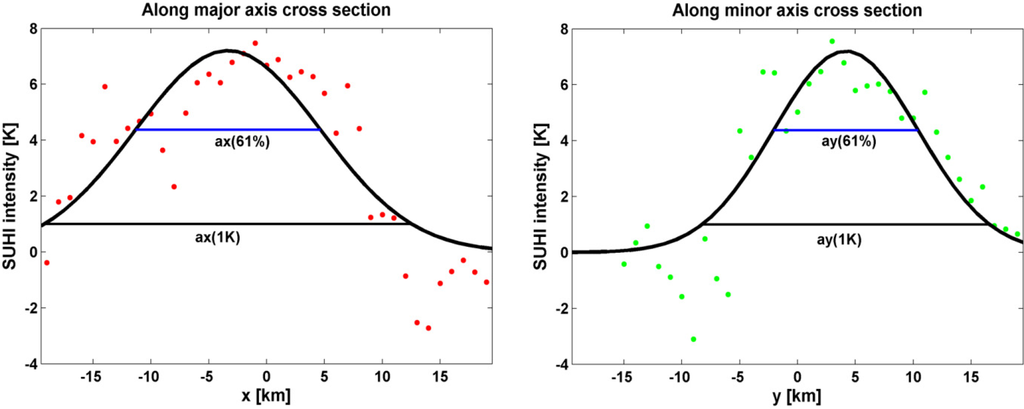
Figure 4. MODIS, August 19, 2009, 14:30. SUHI [K] correspondent to the vertical cross-section of the Gaussian surface along the major axis (left panel) and along the minor axis (right panel). The axes a_x and a_y for the two ellipses of area A_61% and A_1K are also reported.

Figure 4. MODIS, August 19, 2009, 14:30. SUHI [K] correspondent to the vertical cross-section of the Gaussian surface along the major axis (left panel) and along the minor axis (right panel). The axes a_x and a_y for the two ellipses of area A_61% and A_1K are also reported.

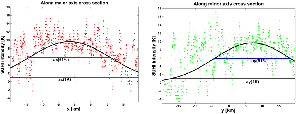
Figure 5. Landsat TM, August 6, 2009, 12:00. SUHI [K] correspondent to the vertical cross- section of the Gaussian surface along the major axis (left panel) and along the minor axis (right panel). The axes a_x and a_y for the two ellipses of area A_61% and A_1K are also reported.

Figure 5. Landsat TM, August 6, 2009, 12:00. SUHI [K] correspondent to the vertical cross- section of the Gaussian surface along the major axis (left panel) and along the minor axis (right panel). The axes a_x and a_y for the two ellipses of area A_61% and A_1K are also reported.

Again, the greater variability of the SUHI values for the high resolution image can be noted, especially if compared with the smoothed cross-sectional curve of the Gaussian surface, that smoothes isolated peaks and is not influenced by localized high/low SUHI values.

6. Conclusions

A fast and robust Gaussian fitting technique was adopted to analyze and parameterize the spatial distribution of the SUHI for a selected urban area. This technique provides a tool to perform quantitative comparisons between different SUHI radial maps useful for inter-city comparisons or for single city analysis over different time scales. The enclosed plotting procedure allows a further better understanding of the shape and orientation of the heat island for each image, and allows us to analyze the performance of the fitting in terms of correlation and reliability of the SUHI pattern representation.

In particular, the results of the parameterization have been shown both for low-resolution and high resolution images. While low-resolution satellite data are adequate for studying the large-scale SUHI characteristics, it is useful for urban planners to use also high-resolution thermal data to monitor the heat island intensity on a smaller scale, with the aim to control or mitigate the effects of the SUHI in relation to population density and land cover.

As expected, an increase of the extent parameters and magnitude and a reduction of the correlation coefficient were observed for the map with the higher spatial resolution. This fitting method is not influenced by localized high surface temperatures within the image, smoothing isolated peaks: this is especially true for the high resolution image, where a greater variability of the SUHI values is evident with respect to the smoothed Gaussian surface, although the effectiveness of the SUHI pattern representation is preserved for the urban area investigated.

References

- Streutker, D.R. A remote sensing study of the urban heat island of Houston, Texas. Int. J. Rem. Sens. 2002, 23, 2595–2608. [Google Scholar] [CrossRef]
- Oke, T.R. City size and the urban heat island. Atmos. Environ. 1973, 7, 769–779. [Google Scholar]
- Oke, T.R. The energetic basis of the Urban Heat Island. Quart. J. Roy. Meteorol. Soc. 1982, 108, 1–24. [Google Scholar]
- Tan, J.; Zheng, Y.; Tang, X.; Guo, C.; Li, L.; Song, G.; Zhen, X.; Yuan, D.; Kalkstein, A.J.; Li, F.; Chen, H. The heat island and its impact on heat waves and human health in Shanghai. Int. J. Biometeor. 2010, 54, 75–84. [Google Scholar]
- Saaroni, H.; Ben-Dor, E.; Bitan, A.; Potcher, O. Spatial distribution and microscale characteristics of the Urban Heat Island in Tel-Aviv, Israel. Landsc. Urban Plan. 2000, 48, 1–18. [Google Scholar]
- Anniballe, R.; Bonafoni, S.; Pichierri, M. Spatial and temporal trends of the surface and air heat island over Milan using Modis data. Rem. Sens. Env. 2014, 150, 163–171. [Google Scholar]
- Anthony, S.M.; Granick, S. Image Analysis with Rapid and Accurate Two-Dimensional Gaussian Fitting. Langmuir 2009, 25, 8152–8160. [Google Scholar] [CrossRef] [PubMed]
- Streutker, D.R. Satellite-measured growth of the urban heat island of Houston, Texas. Rem. Sens. Env. 2003, 85, 282–289. [Google Scholar] [CrossRef]
- Marquardt, D. An algorithm for least square estimation of nonlinear parameters. J. Soc. Indust. Appl. Math. 1963, 11, 431–441. [Google Scholar]
- Dennis, J.E., Jr. Nonlinear Least-Squares. In State of the Art in Numerical Analysis; Jacobs, D., Ed.; Academic Press: New York, NY, USA, 1977; pp. 269–312. [Google Scholar]
- Pichierri, M.; Bonafoni, S.; Biondi, R. Satellite air temperature estimation for monitoring the canopy layer heat island of Milan. Rem. Sens. Env. 2012, 127, 130–138. [Google Scholar]
- Wan, Z. New refinements and validation of the MODIS land-surface temperature/emissivity products. Rem. Sens. Env. 2008, 112, 59–74. [Google Scholar] [CrossRef]
- US Geological Survey (USGS) Center website. Available online: http://earthexplorer.usgs.gov (accessed on 25 March 2015).
- Chander, G.; Markham, B.L.; Helder, D.L. Summary of Current Radiometric Calibration Coefficients for Landsat MSS, TM, ETM+, and EO-1 ALI sensors. Rem. Sens. Env. 2009, 113, 893–903. [Google Scholar]
- Chavez, P.S. Image-based atmospheric correction-revisited and improved. Photogramm. Eng. Rem. Sens. 1996, 62, 1025–1036. [Google Scholar]
- Sobrino, J.A.; Jimenez-Munoz, J.C.; Paolini, L. Land surface temperature retrieval from LANDSAT TM 5. Rem. Sens. Env. 2004, 90, 434–440. [Google Scholar]
© 2015 by the authors; licensee MDPI, Basel, Switzerland. This article is an open access article distributed under the terms and conditions of the Creative Commons Attribution license (http://creativecommons.org/licenses/by/4.0/).