1. Introduction
Tanoak (
Notholithocarpus densiflorus (Hook. & Arn.) Manos, Cannon & S.H.Oh syn.
Lithocarpus densiflorus (Hook. & Arn.) Rehd.) is widespread and abundant in coast redwood (
Sequoia sempervirens (D.Don) Endl.) forests, and is believed to be an integral component of the structure and function of these unique ecosystems [
1,
2,
3]. However, the close association between redwood and tanoak may be relegated to history if sudden oak death (SOD) continues to spread throughout coastal California. This emerging forest disease, which is caused by the exotic pathogen
Phytophthora ramorum S. Werres, A.W.A.M. de Cock, is currently threatening several native tree species, but tanoak is the most severely impacted. Current research indicates drastic declines in tanoak populations and mounting evidence (e.g., field studies, genetic resistance trials, disease progression models) suggests that SOD could eventually drive tanoak toward extinction in redwood forests [
4,
5,
6,
7,
8].
Forest stand structure is often a key determinant of physiognomic resistance, compositional resilience, ecosystem function, wildlife habitat, biodiversity, hydrologic processes, micro-climatic conditions, and regeneration patterns [
9,
10,
11,
12,
13,
14,
15]. Stands with greater vertical and/or horizontal heterogeneity are generally believed to support a higher number of species and to be more productive than compositionally similar stands with more uniform structures [
12,
13,
14], and stands with multiple canopy strata are thought to be
resistant and/or
resilient (sensu [
16]) to a broader spectrum of disturbances than single-stratum stands [
17]. Stand structure influences several hydrological processes [
18,
19,
20,
21], and may have a greater effect on wildlife habitat value than tree species composition; throughout the western United States, northern goshawks (
Accipiter gentilis L.) tend to select stands with large trees and closed canopies, with little apparent concern for the component tree species [
22]. In redwood forests, marbled murrelets (
Brachyramphus marmoratus Gmelin) nest exclusively in tall trees with large limbs, but do not appear to discriminate between redwood and other conifers capable of achieving very large sizes, such as Douglas-fir (
Pseudotsuga menziesii (Mirb.) Franco; [
3]). In general, redwood forests with greater structural diversity are believed to support a greater number of vertebrate species [
3].
While several non-spatial structural attributes (e.g., total basal area, standard deviation of height) have tremendous predictive value, spatially explicit metrics are often necessary to explain ecological processes and functions. Horizontal positioning of trees is particularly predictive of light levels and regeneration patterns [
9,
11], as well as several hydrological phenomena; at similar stocking levels, canopy interception and throughfall rates are affected by the spatial pattern of stems [
9,
15,
21]. Species diversity may also be affected by spatially explicit factors; for example, following timber harvest in western Oregon and Washington states, Luoma
et al. [
23] found that species of ectomycorrhizal fungi differed between dispersed and aggregated retention units. In redwood forests, horizontally heterogeneous stands likely support more species than more homogenous stands, and growth rates of young trees are generally greater in more exposed patches [
3,
24]. However, very few data exist documenting the specific implications of horizontal spatial patterns in redwood ecosystems; such patterns may be particularly complex given the tendency of both redwood and tanoak to produce basal sprouts (especially after disturbance), forming multi-stemmed clumps and contributing to small-scale site persistence [
1,
3,
25].
Despite the widely recognized importance of three-dimensional structural characteristics, and the abundance of tanoak in redwood forests, no previous initiatives have examined the spatially explicit structural relationships between these two species, and very few have considered any structural attributes of tanoak. Tanoak often forms a persistent lower canopy layer in redwood forests [
2,
25], and thus it is likely that tanoak significantly influences overall stand structure. As a prolific producer of large and highly nutritious acorns [
1], the ecological value of tanoak is undeniable, but its structural worth is not well understood. The primary objectives of this study were to examine the current structural impacts of SOD-induced tanoak mortality, predict the immediate impacts of 100% tanoak mortality, and consider the long-term structural impacts of tanoak decline in redwood forests. In addition, we conducted a preliminary exploration of how SOD-induced structural changes compare with typical old-growth characteristics, and how SOD may impact old-growth forests.
2. Methods
Field research was conducted in three different coastal California counties, at sites which contain redwood forest and are infected with P. ramorum. Specific study locations were as follows: Henry Cowell Redwoods State Park (Santa Cruz County), Marin Municipal Watershed District (Marin County), and Humboldt Redwoods State Park (Humboldt County). Within these three sites, we installed a total of 13 plots (23 meter radius; 1/6 hectare) in areas satisfying the following criteria: (a) sufficient redwood coverage (at least 25% redwood canopy cover in all four quadrants of a 1/4 hectare extended plot); (b) between 50 and 200 meters from trails or roads; and (c) slopes less than 60% (31 degrees). Plots were installed within representative areas capturing the extremes of tanoak abundance and disease severity: (a) little or no tanoak [“no-tanoak”; NT]; (b) abundant tanoak with little or no SOD [“healthy”; H]; or (c) abundant tanoak with severe SOD [“diseased”; D]. Areas deemed “representative” were identified as part of previous related research (currently unpublished) by the authors of this paper; suitable areas (which ranged in size from approx. one to three hectares) were subjectively selected (using ocular cover class estimates of tanoak abundance and mortality), but precise plot locations were randomized.
We did not verify the presence of
P. ramorum in our diseased plots, but we are confident that these plots were indeed infected because (a) mortality levels were very high and no other agent is known to cause such severe and widespread mortality of tanoak [
26], (b) presence of the pathogen has been previously confirmed in the general vicinity of all diseased plots [
5,
27,
28], and (c) characteristic symptoms of SOD (see [
8]) were common. Some of our “healthy” plots may also have been infected with
P. ramorum (areas that are entirely unaffected have become very rare at many infected sites), but any resulting tanoak mortality was much lower than in our “diseased” plots. Within our study area, redwood forest with high abundance of hardwoods other than tanoak was very uncommon, and thus our NT plots were located in areas with a small or non-existent hardwood component. Most plots (11) were installed in second-growth forest, but two were installed in old-growth forest in order to facilitate a preliminary examination of variables related to old-growth status. Exact harvest dates could not be determined for all second-growth plots due to incomplete management histories and the tendency of redwood to produce discontinuous growth rings [
29], but all available data indicate that all were harvested in the late 1800s or early 1900s. Key characteristics of all plots are provided in
Table 1.
Table 1.
Key characteristics of sample plots.
Table 1.
Key characteristics of sample plots.
| ID 1 | Plot 2 | County | Status & (% Dead) 3 | Second-growth/Old-growth | Slope Position | Slope (deg) |
|---|
| 1 | HCR-S1 | Santa Cruz | Diseased (49) | Second-growth | Mid | 16 |
| 2 | HCR-S5 | Santa Cruz | No Tanoak | Second-growth | Lower | 15 |
| 3 | HCR-S6 | Santa Cruz | Healthy (10) | Second-growth | Mid | 8 |
| 4 | HRSP-S5 | Humboldt | Healthy (10) | Old-growth | Lower | 14 |
| 5 | HRSP-S7 | Humboldt | Healthy (12) | Second-growth | Lower | 12 |
| 6 | HRSP-S8 | Humboldt | No Tanoak | Second-growth | Alluvial | 2 |
| 7 | HRSP-S9 | Humboldt | No Tanoak | Old-growth | Alluvial | 1 |
| 8 | MMWD-43 | Marin | Diseased (90) | Second-growth | Ridge | 19 |
| 9 | MMWD-S1 | Marin | Healthy (24) | Second-growth | Mid | 22 |
| 10 | MMWD-S2 | Marin | No Tanoak | Second-growth | Ridge | 15 |
| 11 | MMWD-S4 | Marin | No Tanoak | Second-growth | Upper | 17 |
| 12 | MMWD-S7 | Marin | Healthy (21) | Second-growth | Ridge | 10 |
| 13 | MMWD-S9 | Marin | Diseased (74) | Second-growth | Ridge | 18 |
All trees greater than or equal to 10 cm diameter-at-breast-height (dbh) were mapped by recording distance and azimuth from plot center (at breast height), and the following variables were recorded for each tree: species, health status, dbh, height, and height-to-live-crown (hlc). Height and hlc were measured with a Laser Ace hypsometer. Multi-stemmed trees that were split below breast height were counted as separate trees. Crown ratio and crown length were subsequently calculated using height and hlc for each tree. In order to capture recent SOD-induced tanoak mortality, tanoak stems that were broken below breast height were recorded, provided that the fallen bole wood was relatively intact (i.e., it did not compact when stepped upon); in such cases, we estimated pre-death dbh, distance, and azimuth. Dead individuals of other tree species were not recorded if broken below breast height. In order to reconstruct height (for tanoak trees that were dead and broken/fallen) and hlc (for all dead tanoak trees), we used all living tanoak trees in our dataset to construct models fitting height and hlc against dbh. Simple linear models were used for both height and hlc because visual analysis showed such fits to adequately approximate these relationships (i.e., neither curvature nor heteroskedasticy were apparent in residual plots); p and r2 values were, respectively, <0.0001 and 0.53 for height, and <0.0001 and 0.30 for hlc. Height and hlc were not reconstructed for any species other than tanoak because this study focuses specifically on SOD-induced tanoak mortality and, for all other species, the percentage of stems that were dead was very low (e.g., redwood) and/or the total number of occurrences was very low (e.g., pacific madrone, Arbutus menziesii Pursh).
Individual tree-based variables were then used to calculate several plot-level metrics, which included basic structural attributes (simple totals and means), as well as spatially explicit measures of structural complexity: mean nearest neighbor differences (the plot-level mean difference between each tree and its nearest neighbor, with respect to several variables of interest), and the Clark & Evans aggregation index [
11,
30]. The Clark & Evans aggregation index expresses the ratio of the average distance between each tree and its nearest neighbor to the average distance expected under a random distribution of points. For all spatially explicit metrics, we imposed a buffer (
i.e., a guard area) of three meters, meaning that all focal points were required to be at least three meters from the plot boundary, while secondary points (e.g., nearest neighbors) could be selected from all points within the plot.
Data analysis, which relied upon plot-level summary statistics, consisted of comparisons of healthy, diseased, and no-tanoak plots, as well as reconstructed pre-SOD conditions (0% tanoak mortality) and projected future conditions (100% tanoak mortality); in addition, we examined predicted trends over time within each plot. All statistical analyses utilized second-growth plots only (although we also qualitatively explored relationships between second-growth and old-growth plots). We used Tukey’s Honestly Significant Difference (HSD) tests to identify differences among two separate sets of sample groups. The first HSD test (which we refer to as observed) assessed current differences between sampling strata (healthy, diseased, and no-tanoak), and the second HSD test (which we refer to as inferred) assessed differences between the following three groups: reconstructed 0% tanoak mortality plots (healthy and diseased plots combined), projected 100% tanoak mortality plots (healthy and diseased plots combined), and no-tanoak plots. In addition, the difference between 0% and 100% tanoak mortality was calculated for each plot individually, and a one-sample t-test was conducted to determine if these intra-plot differences, collectively, were significantly different from zero (referred to as predicted). Dead stems of species other than tanoak were excluded from all analyses. The statistical software R, version 2.8.0, by The R Foundation for Statistical Computing, was used to conduct all analyses and create all figures; the supplemental package Spatstat, version 1.14-9, was used for all spatially explicit calculations.
Although all of our data were collected in a single field season, we were able to assess structural changes resulting from SOD-induced tanoak mortality. Existing research indicates that the current patchy distribution of SOD in redwood forests, at scales of tens to hundreds of meters, is primarily a result of historical and stochastic factors [
5,
8,
27], as opposed to underlying biotic or abiotic conditions. Therefore, it is likely that consistent differences between healthy and diseased areas are caused by SOD. In contrast, differences between areas with and without tanoak may be controlled by other factors (e.g., soil properties), and thus we do not assert tanoak presence as a causative factor.
3. Results
Many structural variables were significantly related to tanoak presence and/or tanoak mortality (
Table 2). The loss of tanoak should obviously result in an immediate reduction in stem counts and basal area (by a predicted average of 438 stems and 23.8 square meters per hectare), but our results also show that 0% tanoak mortality reconstruction plots tended to have
more stems and
less basal area than plots without tanoak. Similarly, we found that mean dbh was predicted to increase with the loss of tanoak, and that 0% mortality reconstructions had lower mean dbh than 100% mortality projections and plots without tanoak. These findings demonstrate tanoak’s smaller average dbh relative to redwood, as well as its tendency to form dense stands in redwood forests (see
Figure 1,
Figure 2 and
Figure 3 for illustrations of representative second-growth plots in each sampling strata).
Table 2.
Summary of main results. The “
predicted intra-plot changes” column expresses the results of one-sample t-tests assessing whether within-plot differences between 0% and 100% tanoak mortality are significantly different from zero, and if so, the predicted direction of change (see methods section). The number of asterisks indicates the significance level: one symbol = 0.01 < p < 0.05; two symbols = p < 0.01; parentheses indicate borderline significance (0.05 < p < 0.10). The “group comparisons” column displays all significant relationships resulting from Tukey’s HSD tests (see methods section);
inferred (
i) and
observed (
o) relationships are distinguished with parenthetical notations. All analyses consider second-growth plots only. “NN Diffs” is an abbreviation for nearest neighbor differences. Numerical results are provided in the
supplementary material.
Table 2.
Summary of main results. The “predicted intra-plot changes” column expresses the results of one-sample t-tests assessing whether within-plot differences between 0% and 100% tanoak mortality are significantly different from zero, and if so, the predicted direction of change (see methods section). The number of asterisks indicates the significance level: one symbol = 0.01 < p < 0.05; two symbols = p < 0.01; parentheses indicate borderline significance (0.05 < p < 0.10). The “group comparisons” column displays all significant relationships resulting from Tukey’s HSD tests (see methods section); inferred (i) and observed (o) relationships are distinguished with parenthetical notations. All analyses consider second-growth plots only. “NN Diffs” is an abbreviation for nearest neighbor differences. Numerical results are provided in the supplementary material.
| Variable | predicted intra-plot changes
(0% → 100% mort.) | group comparisons
(inferred & observed relationships) |
|---|
| Total Stems | decrease ** | 0% mort. > 100% mort. (i); 0% mort. > no-tanoak (i) |
| Total Basal Area | decrease ** | 0% mort. < no-tanoak (i); 100% mort. < no-tanoak (i); |
| | | diseased < no-tanoak (o) |
| Mean dbh | increase ** | 0% mort. < 100% mort.(i); 0% mort. < no-tanoak (i) |
| Mean Height | increase ** | no significant relationships |
| Mean hlc | increase * | no significant relationships |
| Mean Crown Length | increase * | no significant relationships |
| Mean Crown Ratio | not significant | no significant relationships |
| Mean NN Diffs: dbh | increase * | 0% mort. < 100% mort.(i); 0% mort. < no-tanoak (i) |
| | | healthy < no-tanoak (o); diseased < no-tanoak (o) |
| Mean NN Diffs: Height | increase ** | 0% mort. < no-tanoak (i) |
| Mean NN Diffs: hlc | not significant | no significant relationships |
Mean NN Diffs:
Crown Length | increase * | 0% mort. < no-tanoak (i) |
Mean NN Diffs:
Crown Ratio | (increase) | no significant relationships |
| C&E Aggregation Index | decrease ** | 0% mort. > 100% mort. (i); healthy > diseased (o) |
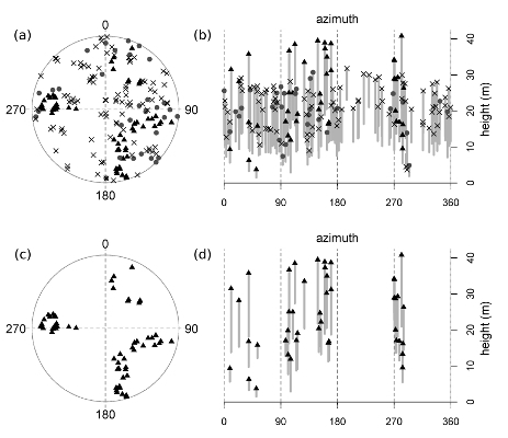
Figure 1.
A representative healthy plot (MMWD-S7; see
Table 1). Trees are mapped (a & c) and represented vertically (b & d; top height and height-to-live-crown are plotted against azimuth, thus “unrolling” the 360 degree view from plot center, and achieving a two-dimensional image by flattening all distances from plot center into a single plane). The top set of graphs (a & b) displays all trees, including reconstructed dead tanoaks, and the bottom set (c & d) illustrates this plot after the removal of all tanoaks (both living and dead). Symbols represent the following: “X”s = dead tanoak; gray circles = living tanoak; black triangles = redwood; open circles = hardwoods other than tanoak; no conifers other than redwood were present in this plot. Gray bars display the length of the live crown (the symbol at the top of each bar is the total tree height and the lower limit of each bar is the height-to-live-crown).
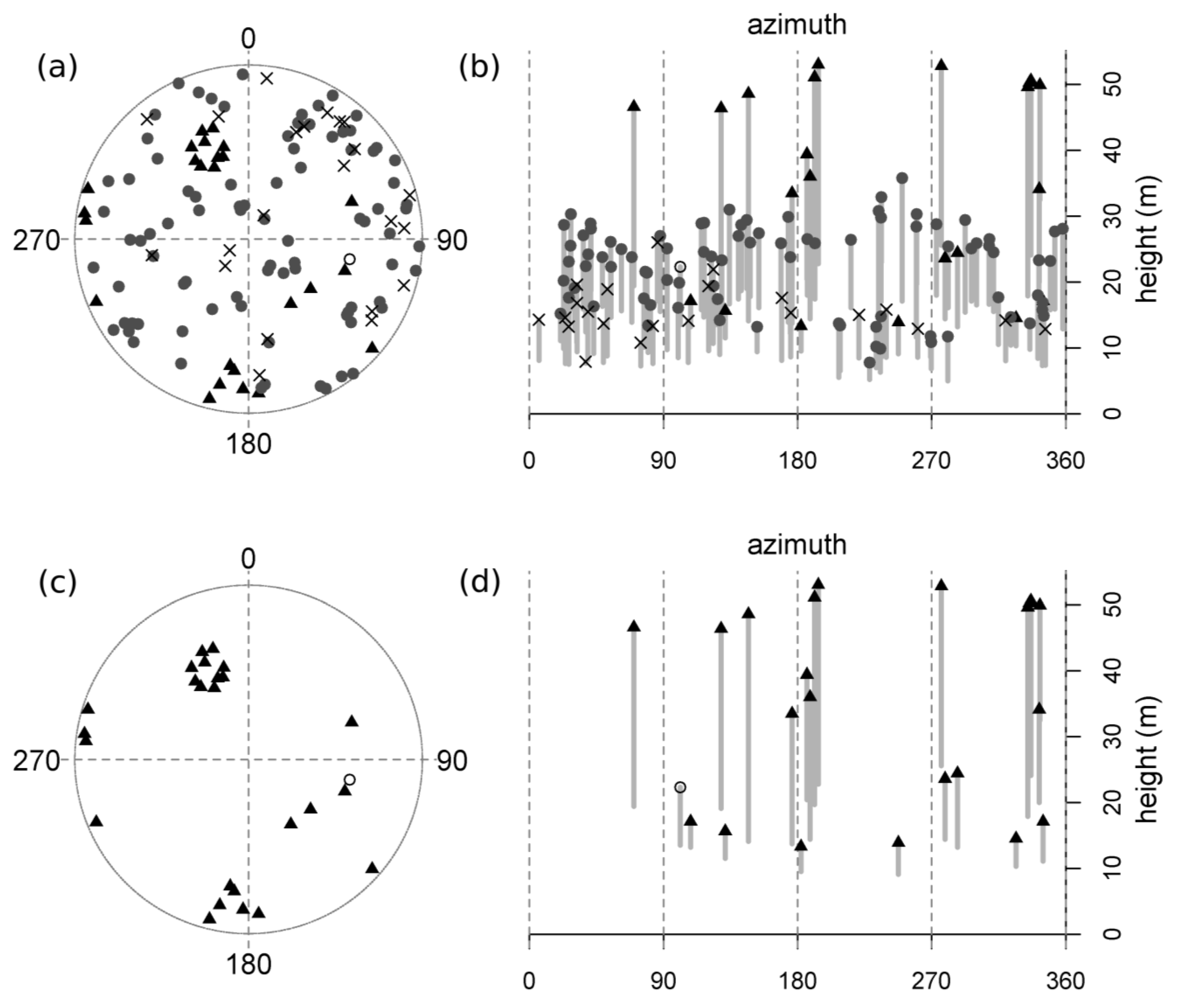
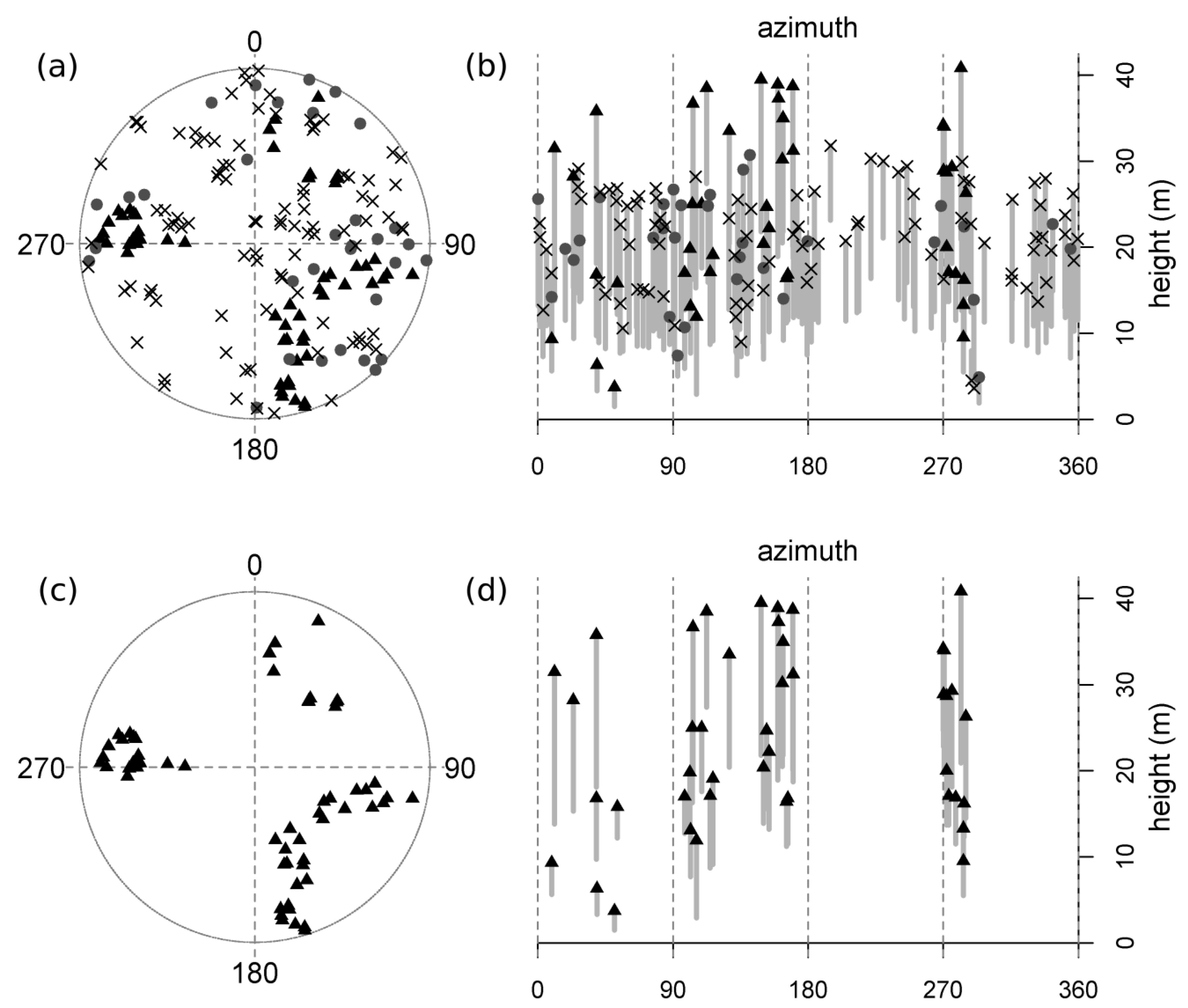
Figure 2.
A representative diseased plot (MMWD-S9; see
Table 1). Trees are mapped (a & c) and represented vertically (b & d; top height and height-to-live-crown are plotted against azimuth, thus “unrolling” the 360 degree view from plot center, and achieving a two-dimensional image by flattening all distances from plot center into a single plane). The top set of graphs (a & b) displays all trees, including reconstructed dead tanoaks, and the bottom set (c & d) illustrates this plot after the removal of all tanoaks (both living and dead). Symbols represent the following: “X”s = dead tanoak; gray circles = living tanoak; black triangles = redwood; open circles = hardwoods other than tanoak; no conifers other than redwood were present in this plot. Gray bars display the length of the live crown (the symbol at the top of each bar is the total tree height and the lower limit of each bar is the height-to-live-crown).
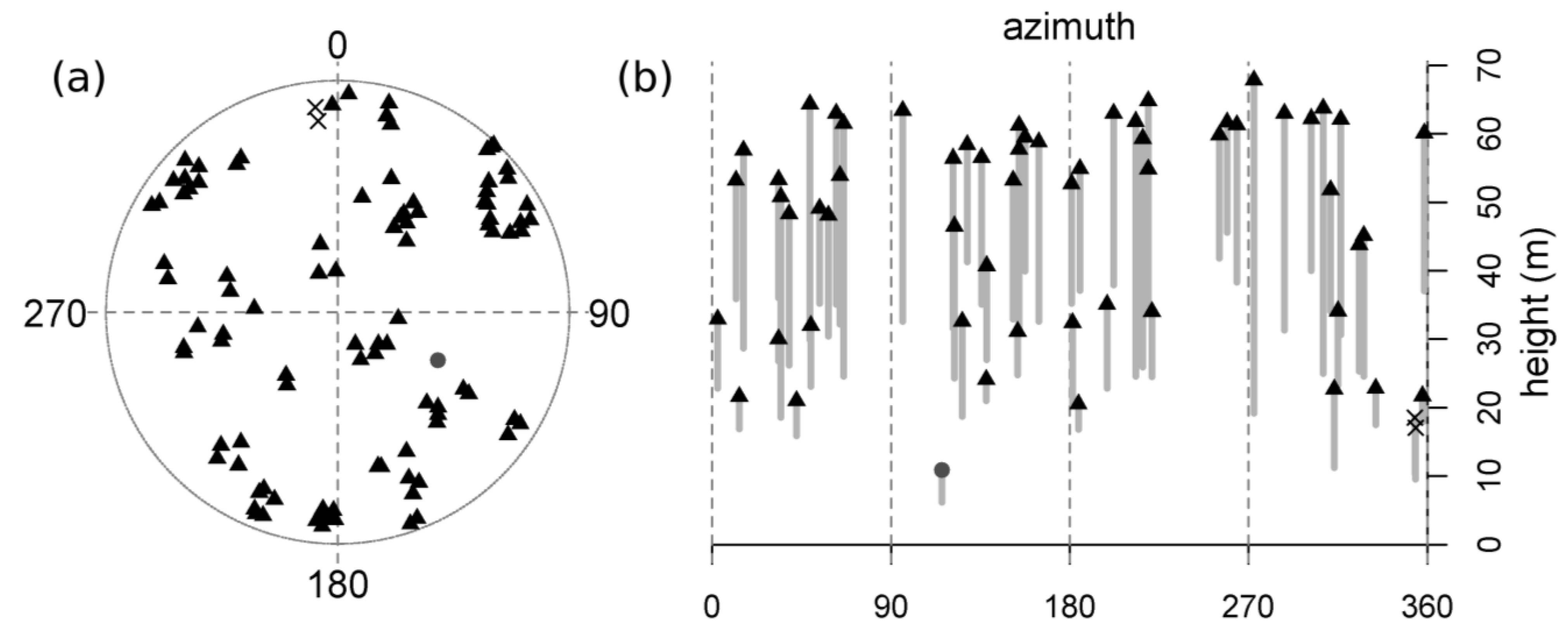
Figure 3.
A representative no-tanoak plot (HCR-S5; see
Table 1). Trees are mapped (a) and represented vertically (b; top height and height-to-live-crown are plotted against azimuth, thus “unrolling” the 360 degree view from plot center, and achieving a two-dimensional image by flattening all distances from plot center into a single plane). Symbols represent the following: “X”s = dead tanoak (reconstructed); gray circles = living tanoak; black triangles = redwood; no other species were present in this plot. Gray bars display the length of the live crown (the symbol at the top of each bar is the total tree height and the lower limit of each bar is the height-to-live-crown).
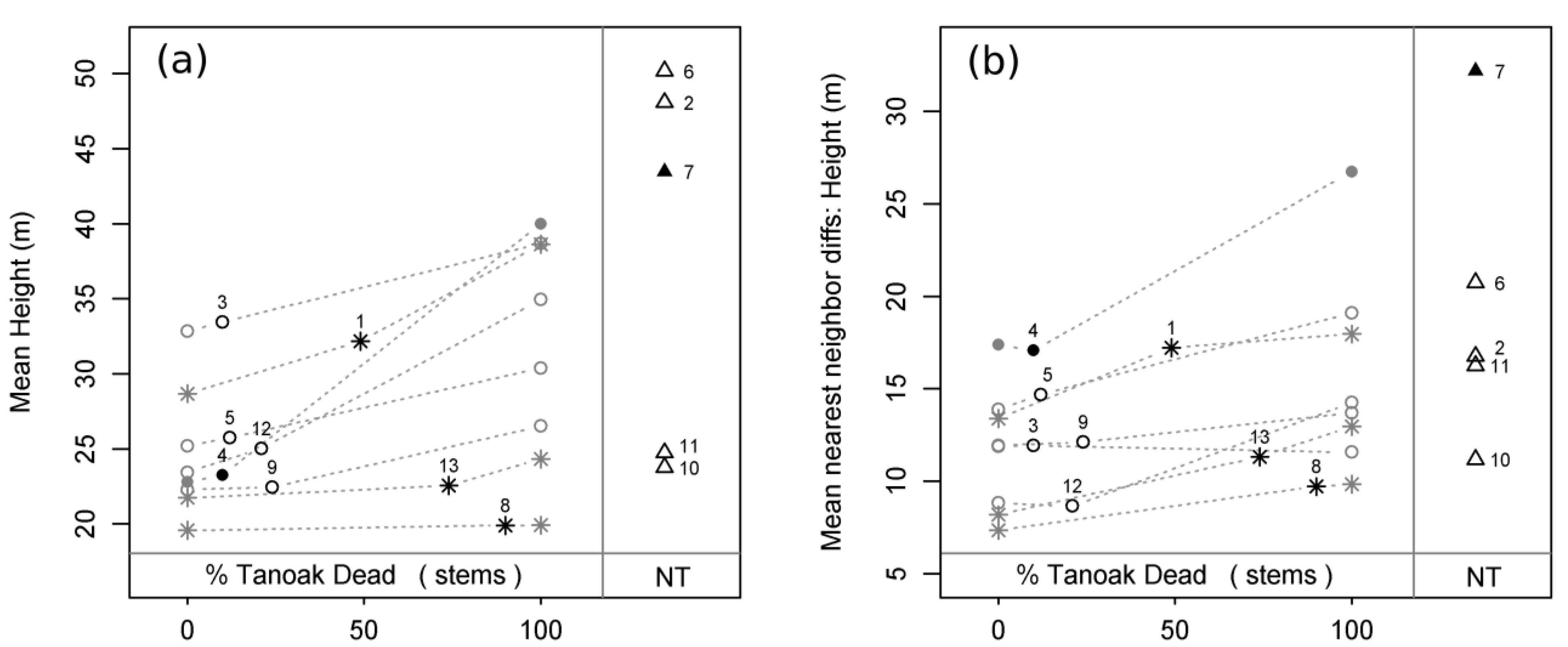
Mean height, mean hlc, and mean crown length increased with the predicted loss of tanoak from our sample plots, but Tukey’s HSD tests failed to detect any differences between observed or inferred groups. As an example, we found that mean tree height within each plot was predicted to increase by an average of 5.7 meters, but because of large variations within each sampling stratum, no differences between groups were apparent (
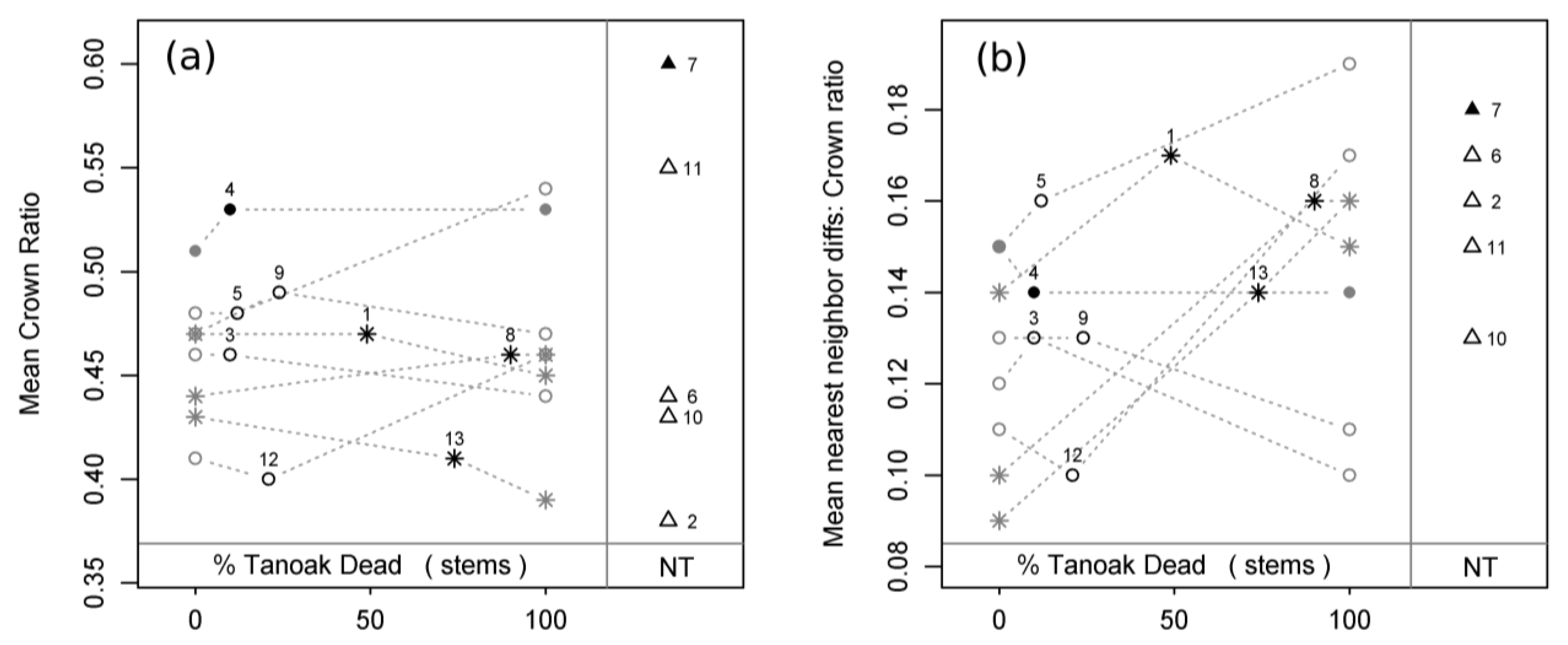
Figure 4a). Mean crown ratio exhibited no observed, inferred, or predicted relationships with tanoak presence or mortality (
Figure 5a).
Several spatially explicit measures of structural complexity were related to tanoak presence and/or SOD-induced tanoak mortality. Mean dbh difference between nearest neighbors was predicted to increase with the loss of tanoak, and 0% mortality reconstructions had lower values than 100% mortality projections and plots without tanoak; in addition, mean dbh difference between nearest neighbors was observed to be higher in no-tanoak plots than in either healthy or diseased plots. Mean nearest neighbor height difference increased with the predicted removal of tanoak, and 0% mortality reconstruction plots had lower values than plots without tanoak (
Figure 4b). Mean crown length difference between nearest neighbors exhibited a qualitatively identical trend to that found for mean height difference between nearest neighbors. Mean hlc difference between nearest neighbors exhibited no observed, inferred, or predicted relationships with tanoak presence or mortality. Observed and inferred mean crown ratio differences between nearest neighbors were similarly non-significant, but there was a borderline positive trend predicted with the loss of tanoak (
Figure 5b).
Figure 4.
Mean height (a) and mean height difference between nearest neighbors (b) as a function of plot status and disease progression. Black numbered symbols represent present conditions of all 13 sampled plots: circles = healthy plots (H); stars = diseased plots (D), triangles = plots without tanoak (NT); open symbols = second growth plots; closed symbols = old growth plots. Grey symbols represent reconstructed pre-SOD conditions (0% tanoak dead) and projected future conditions (100% tanoak dead) for all plots with tanoak. Grey dotted lines connect each plot’s present condition to its respective pre-SOD and future conditions, thereby displaying predicted transitions for each plot. Plot ID numbers correspond to
Table 1.
Figure 5.
Mean crown ratio (a) and mean crown ratio difference between nearest neighbors (b) as a function of plot status and disease progression. Black numbered symbols represent present conditions of all 13 sampled plots: circles = healthy plots (H); stars = diseased plots (D), triangles = plots without tanoak (NT); open symbols = second growth plots; closed symbols = old growth plots. Grey symbols represent reconstructed pre-SOD conditions (0% tanoak dead) and projected future conditions (100% tanoak dead) for all plots with tanoak. Grey dotted lines connect each plot’s present condition to its respective pre-SOD and future conditions, thereby displaying predicted transitions for each plot. Plot ID numbers correspond to
Table 1.
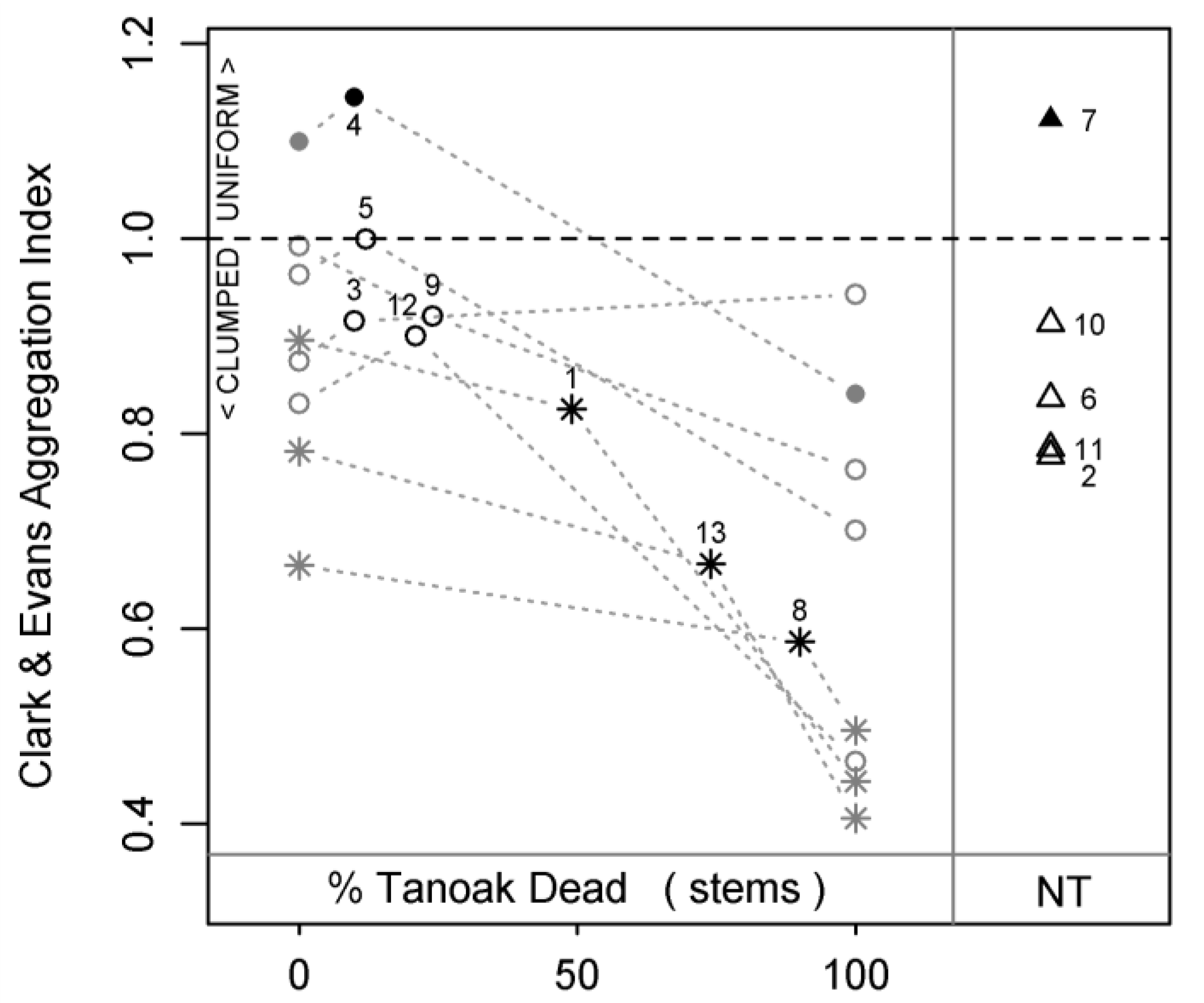
Spatial aggregation of stems was strongly impacted by tanoak mortality. Plots became “clumpier” (lower Clark & Evans aggregation index values) with the predicted loss of tanoak, and 100% mortality projections exhibited more clustering than 0% mortality reconstructions (
Figure 6; these patterns are also clearly evident in figures 1 through 3). Additionally, diseased plots were more clustered than healthy plots, indicating that—unlike most of our predictions—this impact had already occurred at the time of our field measurements. Aggregation of stems within no-tanoak plots was not significantly different from any group with tanoak. In a separate analysis, we found that the removal of redwood did
not increase or decrease “clumpiness” (results not shown), demonstrating that the dispersion of tanoak was essentially random in our study plots (see figures 1 and 2 for representative patterns).
Figure 6.
Clark & Evans aggregation index as a function of plot status and disease progression. Lower index values indicate a greater degree of clustering. Black numbered symbols represent present conditions of all 13 sampled plots: circles = healthy plots (H); stars = diseased plots (D), triangles = plots without tanoak (NT); open symbols = second growth plots; closed symbols = old growth plots. Grey symbols represent reconstructed pre-SOD conditions (0% tanoak dead) and projected future conditions (100% tanoak dead) for all plots with tanoak. Grey dotted lines connect each plot’s present condition to its respective pre-SOD and future conditions, thereby displaying predicted transitions for each plot. Plot ID numbers correspond to
Table 1.
Most variables displayed generally accepted distinctions between old-growth and second-growth redwood forests (
Table 3), demonstrating that our two old-growth plots were fairly representative; for instance, both old-growth plots were less aggregated (higher Clark & Evans values) than comparable (
i.e., H or NT) second-growth plots (
Figure 6), and all nearest neighbor differences were higher in old-growth plots than in most or all comparable second-growth plots (see
Figure 4b and
Figure 5b for examples). Following the predicted loss of tanoak from second-growth redwood forests, the values of most structural variables shifted towards old-growth values (H-OG and/or NT-OG), or exhibited inconsistent relationships with old-growth (H-OG and/or NT-OG). Only one variable, Clark & Evans aggregation index, diverged from both H-OG and NT-OG with the predicted loss of tanoak.
Table 3.
Anecdotal relationships between second-growth and old-growth. In the “Healthy” and “No Tanoak” columns, relationships are displayed for metrics in which all second-growth plot values (within the specified sampling strata) were consistently higher or consistently lower than the old-growth plot. In the “SG to H-OG?” column, “towards” indicates that the removal of tanoak was predicted to shift values of the given metric (for second-growth plots) towards the value of the healthy old-growth plot, while “away” indicates a predicted shift in the opposite direction of the healthy old-growth value. In the “SG to NT-OG?” column, “towards” indicates that the removal of tanoak was predicted to shift values of the given metric (for second-growth plots) towards the value of the no-tanoak old-growth plot, while “away” indicates a predicted shift in the opposite direction of the “no-tanoak” old-growth value. In the “OG vs. SG trend” column, “similar” indicates that the removal of tanoak from the healthy old-growth plot was predicted to have qualitatively identical impacts (i.e., same direction of change) as the removal of tanoak from second-growth plots. Zeros indicate no clear pattern between second-growth and old-growth.
| Variable | Healthy | No Tanoak | SG to
H-OG?
(0% to 100%) | SG to
NT-OG?
(0% to 100%) | OG
vs. SG trend
(0% to 100%) |
|---|
| Total Stems | SG > OG | SG > OG | towards | towards | similar |
| Total Basal Area | 0 | SG < OG | 0 | away | similar |
| Mean dbh | 0 | SG < OG | 0 | towards | similar |
| Mean Height | 0 | 0 | 0 | 0 | similar |
| Mean hlc | SG > OG | 0 | away | 0 | similar |
| Mean Crown Length | 0 | SG < OG | 0 | towards | similar |
| Mean Crown Ratio | SG < OG | SG < OG | 0 | 0 | 0 |
| Mean NN Diffs: dbh | SG < OG | SG < OG | towards | towards | similar |
| Mean NN Diffs: Height | SG < OG | SG < OG | towards | towards | similar |
| Mean NN Diffs: hlc | SG < OG | SG < OG | towards | towards | similar |
| Mean NN Diffs: Crown Length | SG < OG | SG < OG | towards | towards | similar |
| Mean NN Diffs: Crown Ratio | 0 | SG < OG | 0 | 0 | 0 |
| C&E Aggregation Index | SG < OG | SG < OG | away | away | similar |
4. Discussion
Our analyses indicate that several important structural characteristics are likely to be affected by the loss of tanoak from redwood forests, and we were able to detect a current difference in “clumpiness” between healthy and diseased plots. Predicted reductions in total stem counts and total basal area are an obvious immediate impact of SOD-induced tanoak mortality, and predicted instantaneous increases in mean dbh, mean height, mean hlc, and mean crown length are consistent with the larger size of redwood relative to tanoak. However, if new cohorts eventually regenerate in areas experiencing high levels of tanoak mortality (a regenerative response was not evident at the time of field sampling; unpublished data), all of these basic structural attributes may rapidly shift towards their pre-SOD values.
We initially hypothesized that tanoak might be increasing the structural complexity of redwood forests, but we have found no evidence to support this hypothesis. On the contrary, the two measures of vertical complexity that were significantly related to tanoak (mean height difference between nearest neighbors and mean crown length difference between nearest neighbors) indicated decreased diversity when tanoak was present (0% reconstruction as compared to no-tanoak plots), and predicted increases immediately following the loss of tanoak. Similarly, mean dbh difference between nearest neighbors, which could be considered a form of horizontal structural complexity, was negatively affected by tanoak. Plots without tanoak exhibited higher values than healthy plots, diseased plots, and 0% mortality reconstructions, and the loss of tanoak was predicted to result in an immediate increase in mean dbh difference between nearest neighbors. All of these structural complexity metrics should also be affected by future regeneration, but unlike the basic structural attributes discussed above, a new cohort should cause these spatially explicit variables to diverge even farther from their pre-SOD values.
With respect to several attributes (dbh, height, and crown length), average nearest neighbor differences appear to be reduced by the fairly dense lower canopy layer of similarly sized tanoak trees (e.g., figures 1 and 2). However, these metrics of structural diversity may not capture all ecologically relevant structural characteristics; while patches of similarly sized trees will decrease neighbor nearest differences, they may increase other structural quantification metrics (e.g., “patch-types”; sensu [
10]). For instance, the juxtaposition of a plot with a dense sub-canopy layer (e.g.,
Figure 1) and a plot with a less contiguous lower canopy (e.g.,
Figure 3) may be more relevant to some wildlife species than the contrasting characteristics of neighboring trees. Relevant metrics would necessarily require a coarser resolution (spatial grain), rendering any such analyses meaningless—or at least unreliable—at the scale of our plots.
Several observations suggest that SOD-induced tanoak mortality may be accelerating the emergence of old-growth structural attributes in second-growth redwood stands. For example, tanoak mortality should lead to immediate as well as long-term increases in vertical complexity, an attribute that is generally characteristic of old redwood forests [
3,
31]. Our preliminary comparison of second-growth and old-growth plots suggested that, with the removal of tanoak, most structural metrics in second-growth plots should move closer to old-growth values (
Table 3). In addition, another study concluded that SOD-induced tanoak mortality was increasing growth rates and basal sprout regeneration of neighboring redwood trees [
25]. A notable exception to the potential shift towards old-growth characteristics was the predicted and observed increases in clumpiness. Old-growth redwood stands tend to exhibit much more uniform dispersion patterns than second-growth stands, which are characterized by dense clusters of trees surrounding cut stumps [
25,
32]. However, this short-term increase in horizontal structural complexity could lead to a longer-term acceleration towards old-growth characteristics.
Given that the current distribution of SOD is very patchy at many scales, and that the dispersion of tanoak within redwood forests is similarly non-uniform, the structural impacts of SOD may be analogous to a large-scale form of variable density thinning. This method, which aims to increase structural complexity as well as growth rates of residual trees, has been proposed as a strategy to accelerate the transition from second-growth to old-growth in many forest types [
33], including coast redwood [
34]. While the structural impacts of SOD-induced tanoak mortality may therefore be desirable to natural resource managers and casual observers alike, the compositional impacts should be much more unsettling. Tanoak is currently widespread and abundant in old-growth redwood stands, especially on upland sites, and thus the loss of this species is likely to profoundly change the ecology of these forests. If SOD becomes established in old-growth redwood forests, our results suggest that the structural impacts will be similar to the impacts predicted for second-growth forests; for all variables for which the predicted loss of tanoak yielded statistically significant changes within second-growth plots (from 0% mortality reconstructions to 100% mortality projections), predictions for old-growth plots were qualitatively identical. However, all results regarding old-growth plots should be interpreted with caution because only two old-growth plots were sampled and no statistical tests were conducted.
Our inability to observe many significant differences between healthy and diseased plots (in contrast to the large number of significant predictions and inferences) may indicate that many expected changes have yet to occur, but it is also possible that this lack of evidence was due to small sample sizes; for instance, healthy and diseased plots (present condition) consisted of four and three replicates, respectively, while 0% mortality reconstructions and 100% mortality projections consisted of seven replicates each. As such, we have not dismissed the possibility that many expected changes were already occurring at the time of our field measurements. Similarly, structural variables that appeared to be entirely unrelated to tanoak presence and SOD-induced tanoak mortality might have exhibited subtle differences had sample sizes been larger.
Although our reconstructions (0% tanoak mortality prior to SOD) and projections (100% tanoak mortality in the future) test the extremes and may be somewhat unrealistic, these assumptions are within the realm of possibility; background mortality levels for tanoak (
i.e., on uninfected sites) are very low, and SOD-induced tanoak mortality is already approaching 100% in some localized areas ([
27]; unpublished data from related research). However, it is important to emphasize that our 100% tanoak mortality projections assess the structural conditions that would exist if all remaining tanoak trees were to die immediately; in reality it could take many years for projected mortality levels to occur, allowing other trees to recruit in the interim period. Similarly, but with respect to our 0% tanoak mortality reconstructions, some recruitment may have occurred in the time that has passed between tree death and field measurements. It is also worth noting that our models using dbh for vertical reconstruction of dead tanoak stems do not capture all of the variation in height and hlc (r
2 equals 0.53 and 0.30, respectively), and thus reconstructed structural characteristics do not perfectly represent pre-SOD conditions. Depending upon diameter distributions, as well as precise locations of reconstructed tanoaks, estimated height and hlc values could serve to over- or under-estimate the actual structural complexity that existed prior to tanoak mortality. Our inferences and predictions should thus be viewed as a preliminary assessment of the structural changes that may occur as a result of SOD. More complicated procedures (e.g., simulations of disease progression, recruitment, and/or growth responses) could be used in conjunction with our results in order to more accurately forecast future stand structures.
Plots that currently lack tanoak may or may not be representative of the structures that will emerge in the wake of SOD. If tanoak’s current distribution is mostly due to dispersal limitation or stochastic factors, structures similar to those characterizing plots without tanoak may develop in infected areas. However, it is probable that underlying abiotic factors (e.g., soil conditions) and/or disturbance regimes (e.g., floods and silt deposition) affect the abundance of tanoak and other tree species within redwood forests [
1,
35]. As such, we cannot definitely distinguish between the direct effects of tanoak presence and other potentially confounding factors. For instance, if areas where tanoak is currently thriving are inherently supportive of a lower canopy layer of hardwoods or other smaller statured trees, then pre-SOD structures may eventually re-emerge after the loss of tanoak; feasible replacements could include species such as California bay (
Umbellularia californica (Hook. & Arn.) Nutt.), canyon live oak (
Quercus chrysolepis Liebm.), pacific yew (
Taxus brevifolia Nutt.), and pacific madrone. On the other hand, tanoak may be the only tree species with the ability to effectively compete with redwood (
i.e., maintain high relative abundance levels) on some sites. Given this scenario, infected areas would be more likely to acquire structural characteristics that resemble areas currently devoid of tanoak.
Although our data have revealed some interesting patterns, several key questions remain: How long will the immediate structural characteristics of SOD-induced tanoak mortality persist? Will infected stands remain open and aggregated far into the future or will a new cohort of trees quickly establish? Will areas vacated by tanoak begin to resemble areas currently devoid of tanoak, or will entirely new structures emerge? Changes to forest structure have been linked to trophic cascades and various ecosystem processes [
9,
10,
11,
12,
13,
14,
15], and thus these questions should be of great interest to a wide swath of society, encompassing land managers, recreational forest users, and anyone dependent upon ecosystem services from redwood forests. The structural impacts of SOD-induced tanoak decline may be considerable, but the compositional impacts of this emerging disease may be even greater. In redwood forests, total species richness is believed to be higher in areas where other tree species, especially those bearing fruits or nuts, are relatively abundant [
3], and tanoak acorns in particular are known to sustain a wide range of wildlife species [
1]. If tanoak is not replaced by one or more functionally similar tree species (e.g., canyon live oak), redwood forests—which are already relatively poor in tree species—may experience severe reductions in biodiversity; however, it is also important to recognize that diversity could possibly increase as a result of SOD (e.g., if tanoak is replaced by several tree species). The potential for trophic cascades and other compositional impacts, in conjunction with the structural impacts we have documented and/or predicted, suggest that redwood forests are currently experiencing profound and lasting ecological change.


