Contextualizing Mangrove Forest Deforestation in Southeast Asia Using Environmental and Socio-Economic Data Products

Abstract

Research Highlights: This paper provides an alternative approach to contextualize mangrove forest loss by integrating available environmental and socio-economic data sets and products. Background and Objectives: Mangrove forest ecosystems grow in brackish water especially in areas exposed to accumulation of organic matter and tides. This forest type is widely distributed in tropical and subtropical coastal areas. Recent studies have revealed that the mangrove forest ecosystem had significantly degraded due to Land Use and Cover Changes (LUCC) in the recent past. Therefore, contribution of mangrove deforestation drivers has to be assessed to ensure a comprehensive analysis for ecosystem conservation and restoration and facilitate decision making. Materials and Methods: Firstly, a correlation analysis was conducted between individual data products and mangrove deforestation. Each data product was associated with the Dominant Land Use of Deforested Mangrove Patches data for 2012. Next, calculations were performed for specific data combinations to estimate the contributions of anthropogenic factors to mangrove deforestation. Results: In general, our study revealed that 22.64% of the total deforested area was converted into agriculture, 5.85% was converted into aquaculture, 0.69% was converted into infrastructure, and 16.35% was not converted into any specific land use class but was still affected by other human activities. Conclusions: We discovered that the percentage of land affected by these anthropogenic factors varied between countries and regions. This research can facilitate trade-off analysis for natural resources and environmental sustainability policy studies. Diverse management strategies can be evaluated to assess the trade-offs between preserving mangrove forests for climate change mitigation and transforming them for economic purposes.

1. Introduction

Mangrove forest is an ecosystem distributed across coastal zones in equatorial and subtropical regions, mainly between the latitudes of 30° N and 30° S [1,2,3,4,5]. They are strongly influenced by factors such as temperature, currents, insolation, tides, soil, climate, pH, fresh water supply, and salinity [6,7,8]. Recent studies have indicated that mangrove forests sequester more carbon than rainforests [9,10]. Thus, this ecosystem can contribute to carbon emission reduction significantly and can emerge as one of the primary solutions in the global climate change mitigation strategy [8,9,10,11,12,13,14]. However, global mangrove forest cover decreased by 164,600 ha (1.97%) between 2000 and 2012, with an approximate global loss rate of 13,700 ha or 0.16% per year [14]. Previous studies have revealed that this ecosystem has been degraded predominantly by land use and cover change (LUCC) [15,16,17,18,19].

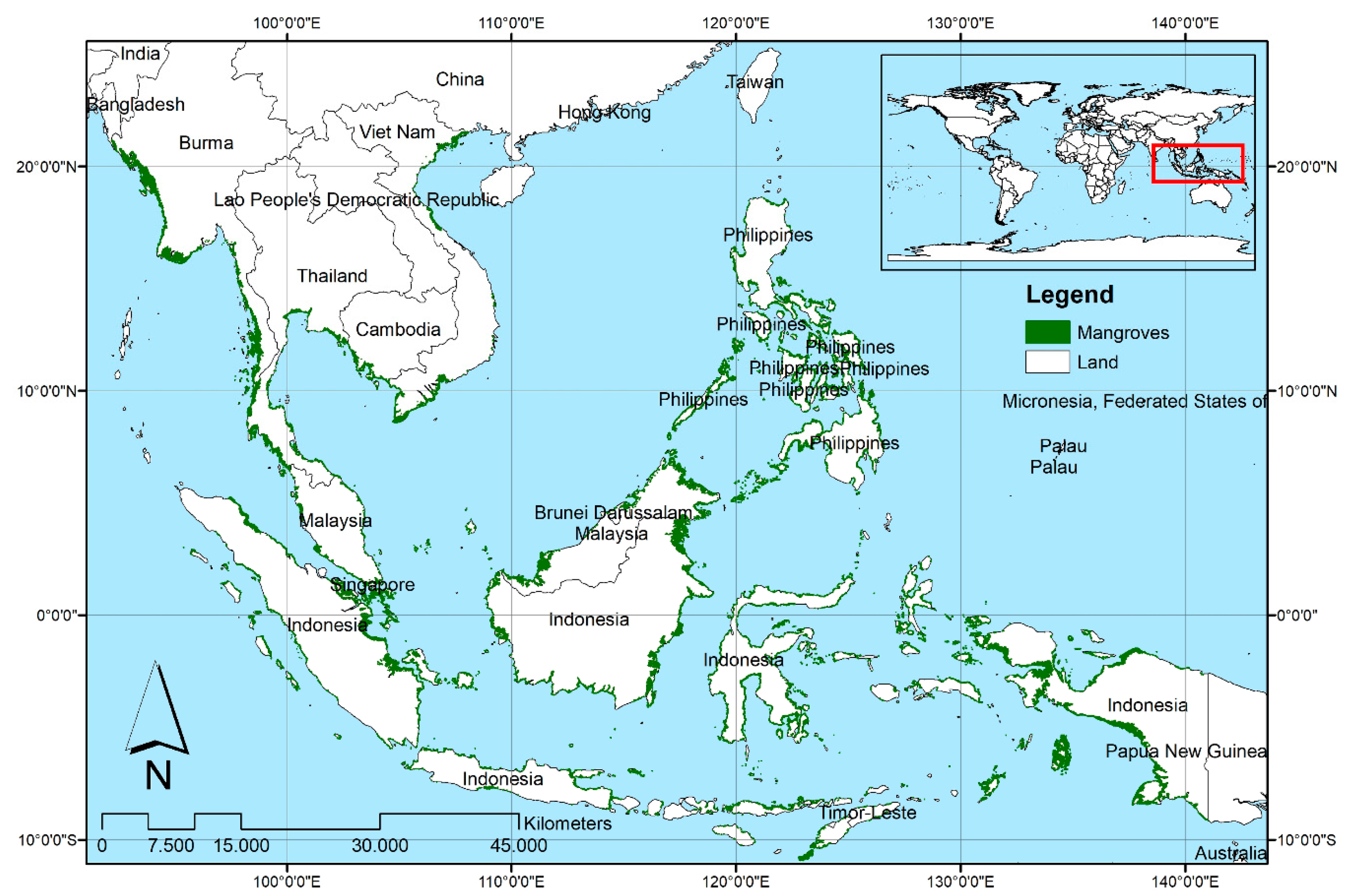
The mangrove forests that grow throughout Southeast Asia (SEA) extend over 4,000,000 ha and constitute 32.2% of the global mangrove area (Figure 1) [20,21]. Mangrove vegetation in SEA is the most diverse in the world and hosts around 268 plant species [22,23,24,25]. However, more than 130,000 ha of mangrove forest in this region were lost between 2000 and 2012 to clearing for fuel wood or charcoal production, rice field and oil palm plantation expansion, conversion to aquaculture, and urban development [25,26,27,28,29,30,31]. Thus, information on mangrove forest loss and its drivers is critical to support decision making by resource managers, planners, and policy makers.

Hamilton and Casey [30,31] mapped the mangrove deforestation rate on a global scale. However, their research did not explore deforestation drivers, which vary between regions. Richards and Friess [30] analyzed the distribution of deforestation drivers in SEA. However, the results generally were only based on dominant land use observations within deforested mangrove forest area interpreted through Landsat images and Google Earth Pro [30]. It is not efficient to apply this approach to such a wide study area. In addition, the results had only 1° spatial resolution. Further, using advanced remote sensing applications and GIS modeling, several global and multi-temporal datasets and products have been proposed (e.g., cropland, urban, population density, and gross domestic production (GDP)) [32,33,34,35,36,37,38], which can provide an alternative approach for evaluating mangrove forest conversion in larger areas.

In this study, we examined various environmental and socio-economic data products to contextualize the main anthropogenic drivers for mangrove forest deforestation in SEA: Agriculture, aquaculture, infrastructure, and other human activities. The analysis was conducted in 10 countries: Indonesia, Myanmar, Malaysia, Thailand, the Philippines, Cambodia, Vietnam, Singapore, Brunei, and Timor Leste. The analysis revealed different characteristics of deforestation in each country. The results of this study will provide guidance for decision makers to consider the appropriate policy for preserving or transforming mangrove forests in specific regions.

2. Materials and Methods

2.1. Mangrove Forests in SEA

SEA experienced deforestation rates of 3.58–8.08% per year from 2000 to 2012, which are notably higher than those in the rest of the world [30]. On a regional scale, the mangrove forests in SEA were the most significantly impacted by anthropogenic activity; the most frequent causes of deforestation were found to be land use conversion into agriculture and aquaculture, followed by clearing, which occurred extensively in this region [24,25,28,29,30,31]. From 2000 to 2012, aquaculture was a major driver of mangrove ecosystem changes. Further, rice cultivation was the dominant driver of mangrove forest loss in Myanmar, and oil palm plantation was the major driver in Malaysia and Indonesia [20].

2.2. Environmental and Socio-Economic Datasets and Products

The input data in this study consisted of recently developed environmental and socio-economic datasets and products, which were computed by integrating several remote sensing and statistic data (

Table 1. Specifications of environmental and socio-economic data products employed in the study.

Data Product	Data Information	Spatial Resolution	Temporal Resolution	Category	Source
MFW	Distribution of Mangroves	30 m	2000	Mangrove	Giri et al. 2011 [5]
DLUDMP	Dominant Land Use	1°	2012	Mangrove	Richards and Friess 2016 [30]
CGMFC-21	Mangrove Forest Cover Loss	30 m	2000 and 2012	Mangrove	Hamilton and Casey 2016 [14]
MCD12Q1	Cropland, Water, and Urban	500 m	2001 and 2012	Environment	Friedl et al. 2015 [32]
MOD44W v6	Water	250 m	2000 and 2012	Environment	Carroll et al. 2017 [33]
HYDE 3.2	Rain-fed and Irrigated Rice	10 km	2000 and 2012	Environment	Goldewijk et al. 2017 [34]
GHS	Built-up	500 m	2000 and 2014	Environment	Pesaresi et al. 2016 [35]
DMSP–OLS v4	Average Lights	30″	2000 and 2012	Socio-economic	National Geophysical Data Center of the National Oceanic and Atmospheric Administration [36]
GDP	Gross Domestic Production	5′	2000 and 2012	Socio-economic	Kummu et al. 2018 [37]
GPW v4	Population Density	30″	2000 and 2015	Socio-economic	Doxsey-Whitfield 2015 [38]

). The different spatial resolutions of the data products were integrated by resampling each data product to a grid cell size equivalent to the lowest resolution of data products involved in the process.

2.2.1. Global Distribution of Mangroves (MFW)

The MFW map generated by Giri et al. [5] was employed. This map has a minimum mapping area of 0.08 ha and presents information about the global distribution of mangrove forests, which are designated as trees and shrubs. The primary data used in the map were produced using Landsat satellite imagery from 1997 to 2000, with 30 m spatial resolution, while the appendix data were based on global, national, and local mangrove databases [5,39].

2.2.2. Dominant Land Use of Deforested Mangrove Patches (DLUDMP) for 2012

Richards and Friess [30] developed the Dominant Land Use of Deforested Mangrove Patches (DLUDMP) dataset, which presented information regarding the dominant land use type in deforested mangrove forests in 2012 for the entire SEA region at a spatial resolution of 1°. The dominant land use type was determined based on the largest land use area, which was calculated using four geographical variables: The normalized difference vegetation index, distance to the main road, and climate suitability indices for oil palm and rice fields, and Google Earth Pro images categorized into eight classes: Fisheries, paddy fields, oil palm plantations, cities, mangrove forests, terrestrial forests, coastal erosion, and classes that were not converted [30].

2.2.3. Continuous Global Mangrove Forests Cover for the 21st Century (CGMFC-21st)

Hamilton and Casey [14] developed CGMFC-21st. This data product presented the annual mangrove forest cover loss from 2000 to 2012, with 30 m spatial resolution. The global forest change (GFC) dataset [40], global distribution of mangroves (MFW) dataset [5], world ecosystem dataset [41], and other appendix spatial data were used to generate the annual global mangrove area between 2000 and 2012 with 30 m spatial resolution [14].

2.2.4. MODIS Land Cover Type Product (MCD12Q1)

Friedl et al. [32] developed MCD12Q1, which presented annual global land cover maps from 2001 to 2017, with 500 m spatial resolution. The classification scheme referred to the International Geosphere-Biosphere Program (IGBP) and could be used as an early warning indicator of global land cover change. The main land cover classes included natural vegetation (11 classes), developed and mosaicked land (3 classes), and non-vegetated land (3 classes) [42]. The main data source was moderate resolution imaging spectroradiometer (MODIS) data for an entire year, wherein observations were conducted every eight days. Additional data included normalized bidirectional reflectance distribution function, adjusted reflectance, and MODIS land surface temperature data. The data were processed using the supervised classification method, which used a high-quality land cover sample database [43,44].

2.2.5. Global MODIS Water Maps Version 6 (MOD44W)

The United States of America produced the Global MODIS Water Maps version 6 (MOD44W) as a part of its National Land Cover Dataset. This data product presented maps of the annual water surface area of the earth from 2000 to 2015 at a spatial resolution of 500 m. The Shuttle Radar Topography Mission Water Body Dataset, with a spatial resolution of 90 m, was the base for the original method. It was averaged to a spatial resolution of 250 m and included in the MODIS sinusoidal tile grid [45]. The algorithm employed to determine the water area was based on the probability of an annual enclosed water area from a 16-day composite of MODIS imagery [46].

2.2.6. History Database of the Global Environment Version 3.2 (HYDE 3.2)

Goldewijk et al. [34] developed the History Database of the Global Environment Version 3.2 (HYDE 3.2), which presented a historical database of human population and time-dependent global land use maps at a spatial resolution of 10 km. In this dataset, cropland was classified into irrigated and rain-fed agriculture and rice fields, which were further classified as irrigated rice and rain-fed rice. Input parameters such as the total area of rain-fed rice per country after 1960 were sourced from the Food and Agriculture Organization (FAO) and the total area of irrigated rice between 1960 and 2010 was obtained by integrating FAO data with the Global Map of Irrigation Areas Version 5 database generated by Siebert et al. [34,47].

2.2.7. Global Human Settlement (GHS)

The GHS was produced by the Joint Research Centre and Directorate-General for Regional Development of the European Commission. This product offered the highest spatial resolution of global settlement datasets available at this scale, and provided multi-temporal information on built-up areas using the Global Land Survey (GLS) archives (1975, 1990, and 2000) and Landsat 8 records for 2013–2014. The built-up data class was obtained through automatic processing using standardized information extraction-based methodologies, which included removing clouds, classification of regions, and mosaicking global data for all four periods [35].

2.2.8. Defense Meteorological Satellite Program–Operational Linescan System (DMSP–OLS)

The National Geophysical Data Center of the National Oceanic and Atmospheric Administration developed the Defense Meteorological Satellite Program–Operational Linescan System (DMSP–OLS). This data product provides multiple nighttime satellite images of the surface of the earth. The DMSP system uses a series of satellite sensors to catch light radiation from the earth at night and observe human habitation, large fishing vessels, and wildfires. The average light is calculated by multiplying the band of average visible light by the frequency proportion of detected light with a spatial resolution of 30″; this can be applied to population density modeling, urban mapping, and assessing localized economic conditions [48,49].

2.2.9. Gross Domestic Product (GDP)

The GDP for 1990 to 2015, computed by Kummu et al. [37], expressed in USD and with a spatial resolution of 5′, was used. The GDP information on data products was computed from the per capita GDP data of all countries obtained from the World Bank Development Indicators database. The gridded GDP data were developed by multiplying the GDP per capita (PPP) by raster data (HYDE 3.2) on the human population for the period between 1990 and 2015, with a grid size of 5′, to produce synchronous datasets that represented official national statistics [37].

2.2.10. Gridded Population of the World Version 4 (GPW)

The Gridded Population of the World (GPW) data was produced by the Socioeconomic Data and Applications Center at the Center for International Earth Science Information Network, Columbia University. This product presented the global distribution of human population (number and density) at a spatial resolution of 30”. The two main sources for this product were non-spatial population data (i.e., tabular data on population numbers in administrative areas) and spatial data based on the administrative areas, which were used to distribute the estimated population data into each 30” grid using the area weighting method [38].

2.3. Methodology

Firstly, correlation analyses were conducted between mangrove deforestation and variations in environmental and socio-economic data products (Figure 2). We overlaid and calculated the area of mangrove forest cover change with changes in environmental and socio-economic data between 2000 and 2012 and assessed their correlation using scatter plot analysis and the Pearson correlation coefficient (r). The technical process in this step also aimed to estimate the converted mangrove area. On overlaying the area where the data products increase with the deforested mangrove area, the converted mangrove area was indicated by the overlaid area. Additionally, compatibility analysis between individual environmental and socio-economic data products and specific classes of DLUDMP data (i.e., rice and oil palm, aquaculture, and urban areas) was conducted using overlay analysis. Compatibility analysis was performed to evaluate the number of grid cells of the DLUDMP data class found in the given data product and this was represented by the degree of consistency (DC), which was computed using Equation (1), as follows:

$$\mathrm{Degree} \mathrm{of} \mathrm{Consistency} \left(\mathrm{DC}\right)= \frac{\mathrm{Number} \mathrm{of} \mathrm{Data} \mathrm{Products} \mathrm{Grid} \left(\mathrm{DPG}\right)}{\mathrm{Number} \mathrm{of} \mathrm{DLUDMP} \mathrm{Grid} \left(\mathrm{DLG}\right)}\times 100\%$$

(1)

The processes were performed in a 1° grid to avoid bias caused by the diverse spatial resolutions of the data products. Each data product was downscaled to a 1° grid size by summing or averaging all the values within the grid. For instance, the CGMFC-21 data, which has a 30 m spatial resolution, was downscaled to 1° spatial resolution. First, we built a grid net with 1° spatial resolution. Then, we intersected this grid net with the CGMFC-21 data and summed the total area within each 1° grid cell. The result is CGMFC-21 data with a 1° spatial resolution, wherein the value of each grid cell was obtained from the sum of 30 m grid cell.

Further, environmental and socio-economic datasets and products were classified into three major deforestation drivers (agriculture, aquaculture, and infrastructure) based on compatibility analysis conducted to assess the accuracy of the parameters in estimating anthropogenic factors. The results are listed in

Table 2. Combinations of environmental and socio-economic parameters used to estimate mangrove deforestation drivers.

Data Product	Data Information	Estimated Land Use Class
MCD12Q1	Cropland	Agriculture
MCD12Q1	Rain-fed Rice	Agriculture
HYDE 3.2	Irrigated Rice	Agriculture
MCD12Q1	Water	Aquaculture
MOD44W	Water	Aquaculture
MCD12Q1	Urban	Infrastructure
GHS	Built-up	Infrastructure
GPW	Population Density	Other Human Activities
GDP	Gross Domestic Product	Other Human Activities
DMSP–OLS	Average Lights	Other Human Activities

.

Further, we used the data combinations presented in Table 2 and logical mathematical functions (Figure A1) to contextualize the drivers of mangrove deforestation, which were categorized into four main classes: Agriculture, aquaculture, infrastructure, and other human activities. The classification results had a spatial resolution of 10 km presented in a spatial resolution of 1°. Each 1° grid cell represented the most dominant driver of mangrove loss, which was computed from the 10 km grid cell using the mode operator (statistics), i.e., the value that appears most often in a set of data.

Furthermore, the accuracy of the results was evaluated by observing 100 sample areas consisting of 50 agriculture class samples, 40 aquaculture class samples, and 10 infrastructure class samples. These were evenly distributed throughout SEA, as highlighted in Figure 3. The deforestation samples were extracted and overlaid onto Google Earth images for an inspection of changes in the field conditions between 2000 and 2012. The changes were manually inspected and visually interpreted, and these changes were defined as when a green mangrove area within a dataset polygon in the image from the year 2000 [5] had transformed into other land cover in the 2012 image, i.e., into land for agriculture, aquaculture, and infrastructure. Lastly, we compared the resulting map with other relevant research and conducted country level analysis.

3. Results

3.1. Correlation between Mangrove Deforestation and Data Products Change

Figure 4 illustrates that the mangrove deforestation area and various environmental and socio-economic data products increased during the study period. In general, agricultural data products (presented in Figure 4a,d,e) such as cropland (MCD12Q1) and rain-fed rice (HYDE 3.2) exhibited high correlations to mangrove deforestation, with respective r values of 0.65 and 0.84. Additionally, irrigated rice (HYDE 3.2) exhibited a low correlation to mangrove deforestation, as indicated by its r value of 0.15. With reference to aquaculture data products (presented in Figure 4b,g), mangrove deforestation exhibited strong positive correlations with the water areas derived from the MCD12Q1 and MOD44W datasets, as indicated by their respective r values of 0.61 and 0.80. Further, the infrastructure data products (presented in Figure 4c,f) indicated that mangrove deforestation exhibited low correlation with urban (MCD12Q1) and built-up (GHS) area increase, as indicated by their respective r values of 0.01 and 0.13. Lastly, assessment of socio-economic data products (presented in Figure 4h,i,j) indicated low correlations between mangrove deforestation and average lights (DMSP–OLS), GDP, and GPW increase, as highlighted by their respective r values of −0.02, −0.04, and −0.06.

In addition to correlation analysis, the spatial distribution and magnitude of the expansion of a particular land use type using environmental and socio-economic data products were plotted, as shown in Figure 5. For instance, the spatial distribution and magnitude of cropland expansion increased in deforested mangrove areas. The magnitude of expansion in deforested mangrove areas was divided into four classes, specifically, <10% (very low), 10–25% (low), 25–50% (medium), and >50% (high), and was measured relative to the mangrove deforestation area in the same grid (a).

3.2. Compatibility between Environmental and Socio-Economic Data Products and Dominant Land Use (DLUDMP) Dataset

The degree of consistency represented the similarity between the data products and DLUDMP data. The DC values highlighted that all the data products exhibited a high consistency; urban areas (MCD12Q1) and irrigated rice (HYDE 3.2) were the only exceptions (

Table 3. Compatibility between data products and Dominant Land Use of Deforested Mangrove Patches (DLUDMP) data.

Data Product	Data Information	DLUDMP Class Data	Number of Data Product Grids	Number of DLUDMP Grids	Degree of Consistency (%)
MCD12Q1	Cropland	Rice and Oil Palm	70	112	62.50
MCD12Q1	Urban	Urban	8	23	34.78
MCD12Q1	Water	Aquaculture	79	102	77.45
HYDE 3.2	Rain-Fed Rice	Rice	18	20	90.00
HYDE 3.2	Irrigated Rice	Rice	7	20	35.00
MOD44W	Water	Aquaculture	101	102	99.01
GHS	Built-Up	Urban	19	23	82.60
DRYAD	Gross Domestic Production	Urban	16	23	69.57
GPW v4	Population Density	Urban	21	23	91.30
DMSP–OLS v4	Average Lights	Urban	21	23	91.30

). These data classes did not register any significant relationships with the DLUDMP data, as also indicated by their correlation to mangrove deforestation. Nevertheless, all data products were utilized to estimate the drivers of the latter.

Each data information type listed in Table 2 was compiled according to the estimated land use class and compared with the DLUDMP data (

Table 4. Degree of consistency between estimated class of mangrove deforestation and DLUDMP data class.

Estimated Land Use Class	DLUDMP Data Class	Number of Data Product Grids	Number of DLUDMP Grids	Degree of Consistency (%)
Agriculture	Rice and Oil Palm	110	112	98.21
Aquaculture	Aquaculture	101	102	99.02
Infrastructure	Urban	20	23	86.96

). Overall, the data combinations indicate fairly accurate performance with degrees of consistency greater than 85%. Thus, the combination of these data products was consistent with the DLUDMP data.

3.3. Mangrove Forest Deforestation Drivers in SEA

Figure 6 illustrates drivers of mangrove deforestation in SEA between 2000 and 2012, divided into nine classes. This deforestation driver types map was prepared with 1° grid cells while the four zoomed-in figures consisted 10 km grid cells. A spatial resolution of 10 km was chosen as it was considered the lowest spatial resolution of the data products used to estimate this product. Intensive agriculture, aquaculture, and infrastructure expansion occurred in several regions. Rakhine, Myanmar, was dominated by agricultural and aquaculture expansion. South Sumatra and Bangka Belitung, Indonesia; the Sabah region, Malaysia; and Merauke, Indonesia, were dominated by significant agriculture expansion. Finally, North Kalimantan, Indonesia, exhibited a notable expansion in aquaculture.

In addition to land conversion drivers, the resulted map provided information about deforestation caused by other human activities. This class can be identified as deforested mangrove areas not converted to a specific land use but accompanied by increases in the population density, night light radiation, and GDP. Areas categorized under the unidentified class were found in small islands in the Philippines and eastern Indonesia.

3.4. Validation Using Google Earth Images

Confusion matrix computation (

Table 5. Confusion matrix of classification. Agri: Agriculture; Aqua: Aquaculture; Infra: Infrastructure; O: Others; TR: Row total; TC: Column total.

		Research Result
		Agri	Aqua	Infra	O	TR
Reference Data	Agri	47	5	1	0	53
	Aqua	0	32	0	0	32
	Infra	0	0	8	0	8
	O	3	3	1	0	7
	TC	50	40	10	0	100

) was used to assess the overall accuracy between the resulted map and Google Earth images for reference. A precision of nearly 87% was obtained.

4. Discussion

4.1. Country Level Analysis

Details of the deforestation area, land use expansion, and deforestation drivers in different SEA countries obtained from this study are listed in

Table 6. Deforested mangrove areas affected by the expansion of various land use types in Southeast Asian countries between 2000 and 2012. Agri: Agriculture; Aqua: Aquaculture; Infra: Infrastructure; OHA: Other human activities; Un: Unidentified.

Country	Agri (ha)	Aqua (ha)	Infra (ha)	OHA (ha)	Un (ha)	Total (ha)
Indonesia	11,006.6738	5192.9245	136.2694	12,765.6505	35,517.8455	64,619.3637
Myanmar	7700.2873	1055.2788	0.0128	0.0000	12,805.9429	21,561.5218
Malaysia	5981.1306	124.4045	543.1067	4775.5530	8587.5523	20,011.7471
Thailand	826.2965	5.8999	83.3874	545.2267	1891.6867	3352.4972
Philippines	84.8971	98.0863	5.1778	323.4811	1571.2900	2082.9323
Cambodia	8.9550	131.7773	0.0000	53.6327	1022.0814	1216.4464
Vietnam	123.8310	43.2550	11.8313	91.4897	445.6410	716.0480
Singapore	8.9948	0.0000	4.2546	17.2777	44.1431	74.6702
Brunei	3.8387	0.0000	0.4444	17.3632	38.4850	60.1313
Timor Leste	1.0454	0.0000	0.1796	0.2398	5.0305	6.4953

.

Figure 7 shows that agriculture expansion affected almost all mangrove forests in all the countries. While aquaculture expansion occurred largely in Indonesia, Myanmar, Philippines, Cambodia, and Vietnam, infrastructure expansion was notable in Malaysia, Thailand, Vietnam, and Singapore.

In general, our study revealed that 22.64% of the total deforested area was converted into agriculture, 5.85% was converted into aquaculture, 0.69% was converted into infrastructure, and 16.35% was affected by other human activities. Unfortunately, 54.47% of the land use change in the total deforested area was unobservable; thus, these changes were classified as unidentified. The high percentage of unidentified areas can be ascribed to two factors. Firstly, the difference between the spatial resolution of the deforestation data (CGMFC-21), which was 30 m, and lower resolution of other data products limited the detection of deforestation drivers in small mangrove forest areas, especially in the Philippines archipelago and eastern Indonesia. This limitation was confirmed by the fact that over 90% of the mangrove forest areas in the unidentified areas were less than 6.25 ha, which was the minimum area that could be detected, based on the highest spatial resolution of the data products applied to estimate the drivers (250 m). Secondly, in addition to anthropogenic factors, the role of naturogenic factors must be inspected further.

4.2. Comparison to Other Research

The obtained map was compared to the results of previous research conducted for the same study period by Richards and Friess [30]. The objectives of the two studies were identical, but the methodologies employed were different. Our research was based on global and multi-temporal datasets, while Richards and Friess’ research was based on dominant land use observations within deforested mangrove areas interpreted through Landsat images and Google Earth Pro [30]. The current study offers at least three improvements related to the classification model, class information, and spatial resolution. In terms of methodology, the approach used in our study increased the efficiency of the process instead of checking mangrove patches individually. In terms of class information, the integration of socio-economic data facilitated the identification of deforested mangrove forest areas affected by other human activities. In the spatial aspect, the resulting map provided better spatial resolution, i.e., 10 km grid cells.

Figure 8 visually highlights that the mangrove forest deforestation driver types exhibited similar trends in both studies. Our method could also detect rice field expansion in western Rakhine, Myanmar; urban development for tourism in southern Bangkok, Thailand; and fishpond expansion in Central Sulawesi, Indonesia.

Figure 9 provides a country-level comparison and reveals that the two sets of results are similar. According to both studies, the dominant deforestation driver in Myanmar, Malaysia, Thailand, and Timor Leste was agricultural land conversion while that in the Philippines and Cambodia was aquaculture land conversion. However, the dominant deforestation drivers identified in the two studies in Indonesia, Vietnam, and Brunei were different. Nevertheless, the two studies yielded compatible results regarding driver characteristics on a regional level. Agricultural land conversion occurred mostly in Myanmar, Malaysia, and Thailand; aquaculture land conversion occurred mostly in Indonesia, the Philippines, and Cambodia; and infrastructural land conversion occurred mostly in Malaysia, Thailand, and Vietnam. However, the two studies yielded slightly different results especially in terms of the percentage contribution of each driver.

The differences between the two studies can, essentially, be attributed to two main factors. Firstly, mangrove deforestation was calculated using CGMFC-21 data in our study, while the research of Richards and Friess was based on GFC data. Therefore, the numbers of deforested areas could have been different. Secondly, global spatial datasets, which have coarse spatial resolution, were utilized in our study. Thus, it was difficult to acquire precise area information. Nevertheless, a regional perspective was employed in this research and the general roles of various deforestation drivers in the SEA region were captured successfully.

5. Conclusions

Mangrove deforestation in SEA was contextualized by inspecting deforestation drivers using recently developed global environmental and socio-economic data products. Regional analysis revealed that agriculture expansion in mangrove forests occurred in all SEA countries. Aquaculture expansion was noted in Indonesia, Myanmar, Philippines, Cambodia, and Vietnam. Further, infrastructure expansion was observed in Malaysia, Thailand, Vietnam, and Singapore. Overall, 22.64% of the mangrove deforestation in SEA between 2000 and 2012 was attributed to agriculture expansion, 5.85% was attributed to aquaculture expansion, 0.69% was attributed to infrastructure expansion, and 16.35% was not converted to any kind of land use type but was indicated as being affected by other human activities.

However, the deforestation drivers in 54.47% of the converted areas could not be identified. Other anthropogenic factors and naturogenic factors such as abrasion, pollution, sedimentation, water balance, climate issue, pests, and diseases must be acknowledged in future studies to improve the accuracy of mangrove deforestation analysis [50,51,52,53,54]. Therefore, additional environmental and socio-economic data products need to be included. Further, the spatial resolution of environment and socio-economic data products applied in this study can be improved. Thus, mangrove deforestation—which is widely distributed spatially and occurs in relatively small areas, as found in many SEA archipelagoes—can be addressed effectively.

The results of this research can facilitate trade-off analysis for natural resources and environmental sustainability policy studies. Diverse management strategies can be evaluated to assess the trade-offs between preserving mangrove forests as climate change mitigation solutions or transforming them for agriculture, aquaculture, and infrastructure to contribute to food security, strengthen commodity exports, and increase economic growth through tourism development.

References

1. Nybakken, J.W. Biologi Laut: Suatu Pendekatan Ekologis; PT. Gramedia: Jakarta, Indonesia, 1988; pp. 363–375. (In Indonesian) [Google Scholar]
2. Romimohtarto, K.; Juwana, S. Biologi Laut, Ilmu Pengetahuan Tentang Biota Laut; Djambatan: Jakarta, Indonesia, 2001; pp. 107–128. (In Indonesian) [Google Scholar]
3. Kathiresan, K.; Bingham, B.L. Biology of mangroves and mangrove ecosystems. Adv. Mar. Biol. 2001, 40, 81–251. [Google Scholar] [CrossRef]
4. Polidoro, B.A.; Carpenter, K.E.; Collins, L.; Duke, N.C.; Ellison, A.M.; Ellison, J.C.; et Elizabeth, J.; Fernando, E.S.; Kathiresan, K.; Koedam, N.E.; et al. The Loss of Species: Mangrove Extinction Risk and Geographic Areas of Global Concern. PLoS ONE 2010, 5, e10095. [Google Scholar] [CrossRef] [PubMed]
5. Giri, C.; Ochieng, E.; Tieszen, L.L.; Zhu, Z.; Singh, A.; Loveland, T.; Duke, N. Status and distribution of mangrove forests of the world using earth observation satellite data. Glob. Ecol. Biogeogr. 2011, 20, 154–159. [Google Scholar] [CrossRef]
6. Chapman, V.J. Mangrove Vegetation; Vaduz J. Cramer: Leutherhausen, Germany, 1976; pp. 319–321. [Google Scholar]
7. Purnobasuki, H. Tinjauan Perspektif Hutan Mangrove; Airlangga University Press: Surabaya, Indonesia, 2005; pp. 36–40. (In Indonesian) [Google Scholar]
8. Alongi, D.M. Introduction in the Energetics of Mangrove Forests; Springer Science and Business Media BV: New York, NY, USA, 2009; pp. 47–64. [Google Scholar]
9. Donato, D.C.; Kauffman, J.B.; Murdiyarso, D.; Krunianto, S.; Stidham, M.; Kaninen, M. Mangroves among the most carbon-rich forests in the tropics. Nat. Geosci. 2011, 4, 293–297. [Google Scholar] [CrossRef]
10. Breithaupt, J.L.; Smoak, J.M.; Smith, T.J. Organic carbon burial rates in Mangrove Sediments: Strengthening the global budget. Glob. Biogeochem. Cycles 2012, 26, 1–11. [Google Scholar] [CrossRef]
11. Murdiyarso, D.; Kauffman, J.B. Addressing Climate Change Adaptation and Mitigation in Tropical Wetland Ecosystems of Indonesia; CIFOR infobrief No. 41; Center for International Forestry Research: Bogor, Indonesia, 2011. [Google Scholar] [CrossRef]
12. Epple, C.; Rangel, S.G.; Jenkins, M.; Guth, M. Managing Ecosystems in the Context of Climate Change Mitigation: A Review of Current Knowledge and Recommendations to Support Ecosystem-Based Mitigation Actions that Look Beyond Terrestrial Forests; Technical Series No.86; Secretariat of the Convention on Biological Diversity: Montreal, QC, Canada, 2016. [Google Scholar]
13. Hu, L.; Li, W.; Xu, B. The role of remote sensing on studying mangrove forest extent change. Int. J. Remote Sens. 2018, 39, 6440–6462. [Google Scholar] [CrossRef]
14. Hamilton, S.E.; Casey, D. Creation of a high spatio-temporal resolution global database of continuous mangrove forest cover for the 21st century (CGMFC-21). Glob. Ecol. Biogeogr. 2016, 25, 729–738. [Google Scholar] [CrossRef]
15. Kathiresan, K.; Rajendran, N. Mangrove ecosystems of the Indian Ocean region. Ind. J. Mar. Sci. 2005, 34, 104–113. [Google Scholar]
16. Gilman, E.; Ellison, J.; Duke, N.; Field, C. Threats to mangroves from climate change and adaptation options: A review. Aquat. Bot. 2008, 89, 237–250. [Google Scholar] [CrossRef]
17. Feka, N.Z.; Ajonina, G.N. Driver causing of mangrove in West-Central Africa: A review. Int. J. Biodivers. Sci. Ecosyst. Serv. Manag. 2011, 7, 217–230. [Google Scholar] [CrossRef]
18. DasGupta, R.; Shaw, R. Mangroves in Asia-Pacific: A Review of Threats and Responses. In Participatory Mangrove Management in a Changing Climate: Perspectives from the Asia-Pacific; DasGupta, R., Shaw, R., Eds.; Disaster Risk Reduction; Springer: Tokyo, Japan, 2017; pp. 1–16. ISBN 978-4-431-56481-2. [Google Scholar]
19. López-Angarita, J.; Tilley, A.; Hawkins, J.P.; Pedraza, C.; Roberts, C.M. Land use patterns and influences of protected areas on mangroves of the eastern tropical Pacific. Biol. Conserv. 2018, 227, 82–91. [Google Scholar] [CrossRef] [Green Version]
20. Spalding, M.; Kainuma, M.; Collins, L. World Atlas of Mangroves; Earthscan: London, UK, 2010; pp. 8–16. [Google Scholar]
21. Bunting, P.; Rosenqvist, A.; Lucas, R.M.; Rebelo, L.; Hilarides, L.; Thomas, N.; Hardy, A.; Itoh, T.; Shimada, M.; Finlayson, C.M. The global mangrove watch—A new 2010 global baseline of mangrove. Remote Sens. 2018, 10, 1669. [Google Scholar] [CrossRef]
22. Giesen, W. Indonesian mangroves part I: Plant diversity and vegetation. Trop. Biodivers. 1998, 5, 99–111. [Google Scholar]
23. Ellison, A.M.; Farnsworth, E.J.; Merkt, R.E. Origins of mangrove ecosystems and the mangrove biodiversity anomaly. Glob. Ecol. Biogeogr. 1999, 8, 95–115. [Google Scholar] [CrossRef] [Green Version]
24. Giesen, W.; Wulffraat, S.; Zieren, M.; Scholten, L. Mangrove Guidebook for Southeast Asia; FAO and Wetlands International: Bangkok, Thailand, 2007; pp. 39–44. [Google Scholar]
25. Navjot, S.S.; Brook, B.W. Southeast Asian Biodiversity in Crisis; Cambridge University Press: New York, NY, USA, 2006; pp. 44–47. [Google Scholar]
26. Primavera, J.H. Overcoming the impacts of aquaculture on the coastal zone. Ocean Coast. Manag. 2006, 49, 531–545. [Google Scholar] [CrossRef]
27. Gopal, B.; Chauhan, M. Biodiversity and its conservation in the Sundarban Mangrove Ecosystem. Aquat. Sci. 2006, 68, 338–354. [Google Scholar] [CrossRef]
28. Hughes, A.C. Understanding the drivers of Southeast Asian biodiversity loss. Ecosphere 2017, 8, e01624. [Google Scholar] [CrossRef]
29. Webb, E.L.; Jachowski, N.R.A.; Phelps, J.; Friess, D.A.; Than, M.M.; Ziegler, A.D. Deforestation in the Ayeyarwady Delta and the conservation implications of an internationally-engaged Myanmar. Glob. Environ. Chang. 2014, 24, 321–333. [Google Scholar] [CrossRef]
30. Ilman, M.; Dargusch, P.; Dart, P.; Onrizal. A historical analysis of the drivers of loss and degradation of Indonesia’s mangroves. Land Use Policy 2016, 54, 448–459. [Google Scholar] [CrossRef]
31. Richards, D.R.; Friess, D.A. Rates and drivers of mangrove deforestation in Southeast Asia, 2000–2012. Proc. Natl. Acad. Sci. USA 2016, 113, 344–349. [Google Scholar] [CrossRef]
32. Thomas, N.; Lucas, R.; Bunting, P.; Hardy, A.; Rosenqvist, A.; Simard, M. Distribution and drivers of global mangrove forest change 1996–2010. PLoS ONE 2017, 12, e0179302. [Google Scholar] [CrossRef] [PubMed]
33. Friedl, M.; Sulla-Menashe, D. MCD12Q1 MODIS/Terra+Aqua Land Cover Type Yearly L3 Global 500m SIN Grid V006 [Data set]. NASA EOSDIS Land Process. DAAC 2015. [Google Scholar] [CrossRef]
34. Carroll, M.L.; DiMiceli, C.M.; Wooten, M.R.; Hubbard, A.B.; Sohlberg, R.A.; Townshend, J.R.G. MOD44W MODIS/Terra Land Water Mask Derived from MODIS and SRTM L3 Global 250m SIN Grid V006 [Data set]. NASA EOSDIS Land Process. DAAC 2017. [Google Scholar] [CrossRef]
35. Goldewijk, K.K.; Beusen, A.; Doelman, J.; Stehfest, E. Anthropogenic land-use estimates for the Holocene—HYDE 3.2. Earth Syst. Sci. Data 2017, 9, 927–953. [Google Scholar] [CrossRef]
36. Pesaresi, M.; Ehrlich, D.; Ferri, S.; Florczyk, A.J.; Freire, S.; Halkia, S.; Julea, A.M.; Kemper, T.; Soille, P.; Syrris, V. Operating Procedure for the Production of the Global Human Settlement Layer from Landsat Data of the Epochs 1975, 1990, 2000, and 2014; Publications Office of the European Union EUR 27741 EN: Ispra, Italy, 2016. [Google Scholar] [CrossRef]
37. Version 4 DMSP-OLS Nighttime Lights Time Series. Available online: https://ngdc.noaa.gov/eog/dmsp/downloadV4composites.html (accessed on 8 August 2019).
38. Kummu, M.; Taka, M.; Guillaume, J.H.A. Gridded global datasets for Gross Domestic Product and Human Development Index over 1990–2015. Sci. Data 2018, 5, 180004. [Google Scholar] [CrossRef]
39. Doxsey-Whitfield, E.; MacManus, K.; Adamo, S.B.; Pistolesi, L.; Squires, J.; Borkovska, O.; Baptista, S.R. Taking Advantage of the Improved Availability of Census Data: A First Look at the Gridded Population of the World, Version 4. Pap. Appl. Geogr. 2015, 1, 226–234. [Google Scholar] [CrossRef]
40. FAO. The World’s Mangroves 1980–2005; Forestry Paper FAO 153; Food and Agriculture Organization of the United Nations: Rome, Italy, 2007; pp. 21–27. [Google Scholar]
41. Hansen, M.C. High-Resolution Global Maps of 21st-Century Forest Cover Change. Science 2013, 342, 850–853. [Google Scholar] [CrossRef] [Green Version]
42. Olson, D.M.; Dinerstein, E.; Wikramanayake, E.D.; Burgess, N.D.; Powell, G.V.N.; Underwood, E.C.; D’amico, J.A.; Itoua, I.; Strand, H.E.; Morrison, J.C.; et al. Terrestrial Ecoregions of the World: A New Map of Life on Earth: A new global map of terrestrial ecoregions provides an innovative tool for conserving biodiversity. BioScience 2001, 51, 933–938. [Google Scholar] [CrossRef]
43. Friedl, M.A.; Menashe, D.S.; Tan, B.; Schneider, A.; Ramankutty, N.; Sibley, A.; Huang, X. MODIS Collection 5 global land cover: Algorithm refinements and characterization of new datasets. Remote. Sens. Environ. 2010, 114, 168–182. [Google Scholar] [CrossRef]
44. Quinlan, J.R. C4.5: Programs for Machine Learning; Morgan Kaufmann Publishers, Inc.: San Mateo, CA, USA, 1993; pp. 71–72. [Google Scholar]
45. Freund, Y. Boosting a weak learning algorithm by majority. Inf. Comput. 1995, 121, 256–285. [Google Scholar] [CrossRef]
46. Carroll, M.; Townshend, J.R.; DiMiceli, C.M.; Noojipady, P.; Sohlberg, R. A New Global Raster Water Mask at 250 M Resolution. Int. J. Digit. Earth 2009, 2, 291–308. [Google Scholar] [CrossRef]
47. Carroll, M.L.; DiMiceli, C.M.; Townshend, J.R.G.; Sohlberg, R.A.; Elders, A.I.; Devadiga, S.; Sayer, A.M.; Levy, R.C. Development of an operational land water mask for MODIS Collection 6, and influence on downstream data products. Int. J. Digit. Earth 2016, 10, 207–218. [Google Scholar] [CrossRef]
48. Siebert, S.; Kummu, M.; Porkka, M.; Döll, P.; Ramankutty, N.; Scanlon, B.R. A global data set of the extent of irrigated land from 1900 to 2005. Hydrol. Earth Syst. Sci. 2015, 19, 1521–1545. [Google Scholar] [CrossRef] [Green Version]
49. Elvidge, C.D.; Erwin, E.H.; Baugh, K.E.; Ziskin, D.; Tuttle, B.T.; Ghosh, T.; Sutton, P.C. Overview of DMSP nighttime lights and future possibilities. In Proceedings of the Urban Remote Sensing Joint Event, Shanghai, China, 20–22 May 2009. [Google Scholar] [CrossRef]
50. Zhou, Y.; Smith, S.J.; Zhao, K.; Imhoff, M.; Thomason, A.; Bond-Lamberty, B.; Asrar, G.R.; Zhang, X.; Elvidge, C. A global map of urban extent from nightlights. Environ. Res. Lett. 2015, 10, 1–11. [Google Scholar] [CrossRef]
51. Krauss, K.W.; Lovelock, C.E.; McKee, K.L.; López-Hoffman, L.; Ewe, S.M.L.; Sousa, W.P. Environmental drivers in mangrove establishment and early development: A review. Aquat. Bot. 2008, 89, 105–127. [Google Scholar] [CrossRef]
52. Maiti, S.K.; Chowdury, A. Effects of Anthropogenic Pollution on Mangrove Biodiversity: A Review. J. Environ. Prot. 2013, 4, 1428–1434. [Google Scholar] [CrossRef] [Green Version]
53. Alongi, D.M. The Impact of Climate Change on Mangrove Forests. Curr. Clim. Chang. Rep. 2015, 1, 30–39. [Google Scholar] [CrossRef]
54. Osorio, J.A.; Casparus, J.; Crous, M.J.; Wingfield, Z.; Beer, W.D.; Roux, J. An assessment of mangrove diseases and pests in South Africa. For. Int. J. For. Res. 2017, 90, 343–358. [Google Scholar] [CrossRef]
Figure 1. The study area includes mangrove forests in 10 Southeast Asian countries: Thailand, Myanmar, Vietnam, Cambodia, Malaysia, the Philippines, Brunei, Singapore, Indonesia, and Timor Leste. The forest distribution is in accordance with the Mangrove Forest of the World (MFW) datasets generated by Giri et al. [5].
Forests 10 00952 g001
Figure 2. Flowchart of the research methodology.
Forests 10 00952 g002
Figure 3. Sample area distribution (source: Google Earth Pro).
Forests 10 00952 g003
Figure 4. Scatter plot of the relationship between mangrove deforestation and the changes in environmental and socio-economic data products from 2000 to 2012 based on Continuous Global Mangrove Forests Cover for the 21st Century (CGMFC-21) data. Increases in (a) cropland area, (b) water area, and (c) urban area from 2001 to 2012 based on MODIS Land Cover Type Product (MCD12Q1) data; (d) rain-fed rice and (e) irrigated rice from 2000 to 2012 based on History Database of the Global Environment Version 3.2 (HYDE 3.2) data; (f) water area increase from 2000 to 2012 based on Global MODIS Water Maps Version 6 (MOD44W) data; (g) built-up area increase from 2000 to 2014 based on Global Human Settlement (GHS) data; (h) population density increase from 2000 to 2015 based on Gridded Population of the World Version 4 (GPW) data; (i) Gross Domestic Product (GDP) increase from 2000 to 2012; and (j) average lights increase from 2000 to 2012 based on Defense Meteorological Satellite Program–Operational Linescan System (DMSP–OLS) data. Each point represents the number of 1° grids that registers an increase in mangrove deforestation and data products. These increases were calculated for each grid cell in overlapping positions to represent the area of mangrove forest affected by the increase in each data product.
Forests 10 00952 g004
Figure 5. Spatial distribution of increased percentages of (a) cropland, (b) water (MCD12Q1), (c) built-up areas, and (d) population density in deforested mangrove areas. In southern Vietnam, the deforestation rate is low and cropland increase is relatively high while in northern Kalimantan, the deforestation rate is high and cropland increase is relatively low. Thus, it can be understood that cropland increase is the primary drivers for deforestation in southern Vietnam, while cropland increase is not among the main drivers for deforestation in northern Kalimantan.
Forests 10 00952 g005
Figure 6. (a) Mangrove forest deforestation driver types map with 10 km grid cell resolution. The highlighted deforested zones are: (b) Rakhine, Myanmar, with 10 km grid cell resolution; (c) South Sumatera and Bangka Island, Indonesia, with 10 km grid cell resolution; (d) Sabah, Malaysia, and North Borneo, Indonesia, with 10 km grid cell resolution; and (e) Merauke, Indonesia, with 10 km grid cell resolution. Map of mangrove forest deforestation driver types in Southeast Asia (SEA) between 2000 and 2012. Agri stands for agriculture, Aqua stands for aquaculture, Infra stands for infrastructure, and OHA stands for other human activities. The combined classes are represented using &, e.g., “Agri & Aqua” stands for agriculture and aquaculture, indicating that there are two types of mangrove forest drivers in one grid.
Forests 10 00952 g006
Figure 7. Contributions of mangrove deforestation drivers to the total mangrove deforestation area in each country.
Forests 10 00952 g007
Figure 8. Comparison of mangrove deforestation driver types assessed in this study (a) with the DLUDMP dataset (b). Visual analysis of three types of highlighted land use expansion: (c) Agriculture, (d) infrastructure or urban, and (e) aquaculture.
Forests 10 00952 g008
Figure 9. Comparison of the results of the current study with those of Richards and Friess [30] for three main deforestation driver classes. The Agriculture, Aquaculture, and Infrastructure classes correspond to the results of the current study while the Rice & Oil Palm (R&F), Aquaculture (R&F), and Urban (R&F) classes correspond to Richards and Friess [30] and were used for comparison. The percentage of each driver refers to the total deforestation area for each country between 2000 and 2012. The countries are ordered by their total mangrove forest loss during the period.
Forests 10 00952 g009