The Variation Driven by Differences between Species and between Sites in Allometric Biomass Models


1
Department of Silviculture, Transilvania University of Brasov, 1 Șirul Beethoven, 500123 Brașov, Romania
2
Buckinghamshire New University, Queen Alexandra Rd, High Wycombe HP11 2JZ, UK
Forests 2019, 10(11), 976; https://doi.org/10.3390/f10110976
Submission received: 3 September 2019
/
Revised: 24 October 2019
/
Accepted: 1 November 2019
/
Published: 4 November 2019
(This article belongs to the Section Forest Ecology and Management)
Abstract
:Background and Objectives: It is commonly assumed that allometric biomass models are species-specific and site-specific. However, the magnitude of species and site dependency in these models is not well-known. This study aims to investigate the variation in allometric models (i.e., aboveground biomass predicted by diameter at breast height and tree height) that has originated from the differences between tree species and between sites, thereby contributing to a better understanding of species and site-specificity issue in these models. Materials and Methods: The study is based on two large biomass datasets of 4921 and 5199 trees, from Eurasia and Canada. Using a nested ANOVA model on relative aboveground biomass residuals (with species and site as random effects), the proportion of variance explained by species or site was assessed by means of Variance Partition Coefficient (VPC). Results: The proportion of variance explained by species (VPCspecies = 42.56%, SE = 6.10% for Dataset 1 and VPCspecies = 47.54%, SE = 6.07% for Dataset 2) was larger than that explained by site (VPCsite = 20.08%, SE = 3.35% for Dataset 1 and VPCsite = 8.27%, SE = 1.38% for Dataset 2). The proportion of variance explained by site decreased by 24%–44% and the proportion of variance explained by species changed only slightly, when height is included in the allometric biomass models (i.e., models based on diameter at breast height alone, compared to models based on diameter at breast height and tree height). Conclusions: Allometric biomass models were more species-specific than they were site-specific. Therefore, the species (i.e., differences between species) seems to be a more important driver of variability in allometric models compared to site (i.e., differences between sites). Including height in allometric biomass models helped reduce the dependency of these models, on sites only.

1. Introduction
Allometric biomass models are key components for any forest GHG (greenhouse gas) inventory [1,2]. These are regression models that use tree dimensions, such as diameter at breast height (D, at 1.3 m from the ground) and/or tree height (H) to predict aboveground biomass (AGB) [3]. The power-law function (AGB = αDβ) [4] is a widely accepted form of allometric biomass model. Despite the allometric scaling theory, which support an invariant allometric scaling (the scaling exponent β = 8/3) [5,6], there is little support from empirical evidence for this theory [7,8].
It is well-known that allometric biomass models vary by species [7,9,10] and by site [10,11]. As tree architecture and wood density (which define tree allometry) are genetically controlled [12,13], it is expected that allometry would differ between species. The allometry of trees (defined here as the relationship between aboveground biomass and tree diameter and/or height) is the result of the interaction between endogenous growth processes and exogenous constraints exerted by the environment [14]. Therefore, allometric biomass models are expected to be altered by environmental conditions, which vary from site-to-site.
The environmental factors that define the site conditions, and which affect allometric biomass models are: (i) Soil properties, (ii) climate conditions, and (iii) current and past competition [10]. It was demonstrated that soil fertility (nutrients and water) can modify the allocation of biomass [15,16]. Among soil properties that were shown to influence allometry are, the cation exchange capacity and carbon to nitrogen ratio [17], salinity, and compaction [18]. Besides soil, the climate conditions (irradiance, precipitation, temperature, and atmospheric composition, such as enhanced CO2) were also reported to alter biomass allocation among tree organs [2,18,19]. Additionally, when in different stages of development, the trees were shown to have different allometries [20,21]. Competition between trees modifies the H-D ratio and crown size [22] with direct consequences on aboveground biomass allometry. This was confirmed by a study on allometry of dominant and supressed trees [23]. As trees do not respond very quickly to changes in competition, it is not only the current tree competition that is important, but also previous competition [10]. The type of mixture, exposing different levels of interspecific competition were shown to affect aboveground biomass allometry [24]. Furthermore, competition (intraspecific and interspecific) can be adjusted through measures of forest management. For example, thinning reduces competition between trees being proven to reduce the ratio between fine roots and leaf biomass [25]. Also, in even-aged stands, the patterns of tree competition are different compared to uneven-aged stands, where greater structural diversity may result in more diverse tree allometries. However, all these factors affecting allometry usually interact with each other, and also with the genotype. Therefore, including such factors as a fixed effect variable in allometric models, often give poor results. By considering the site only, as a vector of all these effects (main effects and their interactions) seems to be a more practical approach [2].
Because allometric biomass models are species- and site-specific and because measuring biomass is a very laborious operation, an important and pressing question for practice is how transferable these models are (from one species to another and from one site to another). Knowing the magnitude of species- and site-specificity would tell whether the transfer could be done with insignificant costs regarding prediction accuracy loss, or not. There was an intense focus lately in comparing generic allometric models with site-specific models [26,27,28,29,30,31,32,33]. Therefore, there is a strong interest in gaining a deeper understanding of species- and site-dependency of allometric biomass models. A straightforward and easy way to investigate this issue is to check the proportion of variance that is explained by differences between species and differences between sites. The intuition is simple: A very small proportion of variance that is explained for example by ‘site’ would indicate that there is much more variability within sites than between. Since the differences between sites are small, the cost (on prediction accuracy) associated with the transfer of an allometric model from one site to another would also be small. A large proportion, on the other hand, would indicate that transfers of allometric models should be avoided.
The magnitude of species- and site-specificity in allometric biomass models is not well known. Therefore, using two large biomass datasets, this paper investigated, (i) the proportion of variance that was caused by differences between species and between sites, (ii) how the proportion of variance explained by species and site changes when adding height as additional predictor of aboveground biomass, and (iii) the species and site random effects.
2. Materials and Methods
2.1. Biomass Data
To reliably assess the random effects of species and sites in allometric biomass models, two large biomass datasets [34,35,36] were used, containing observations of forest trees (Table 1). Dataset 1 [34] contains 9613 trees sampled from Europe and Asia, whereas Dataset 2 [35,36], 9808 trees sampled from Canada. The ‘site’ as used in this study represents a delimitation of a geographical area characterized by common conditions regarding soil and climate. Because the location name was not provided for all trees, the trees were grouped by ‘site’, based on their geographical coordinates. Although, latitude and longitude were provided for each tree, the coordinates describe the location of the site (e.g., forest stand, plot) and not the location of individual trees. Therefore, the trees sharing similar latitude and longitude were grouped in a ‘site’. The precision of latitude and longitude was 0.01 decimal degrees (i.e., 787.1 m at 45° N and 435.0 m at 67° N) for Dataset 1 and 0.001 decimal degrees (i.e., 78.7 m at 45° N and 43.5 m at 67° N) for Dataset 2.
Both datasets were prepared for analysis: (i) All trees lacking one or more of the measurements for diameter at breast height (D), tree height (H), and aboveground biomass (AGB), latitude and longitude were removed (i.e., 3175 observations were removed from Dataset 1 and 3629 from Dataset 2); (ii) all trees with D < 5 cm were removed, because they represent a small share of total biomass and because they would dominate the regression line [2] (i.e., 1320 observations were removed from Dataset 1 and 770 from Dataset 2); (iii) all categories (species or sites) with less than 5 trees per category were removed, in order to reliably assess the parameter estimates and random effects [37] (i.e., 186 observations were removed from Dataset 1 and 192 from Dataset 2); (iv) the outliers were removed (i.e., 11 observations from Dataset 1 and 18 from Dataset 2 were removed; the outliers were identified as observations that correspond to residuals which fall outside the interval described by ±3 standard deviations).
Both datasets showed a comparable range for the number of trees per species and trees per site (Table 1). The distribution of number of trees per species (Figure 1a) was slightly different for Dataset 1 and 2. For Dataset 1, there was a larger number of species with relatively low number of trees per species (35 species out of 56 had less than 20 trees per species). For Dataset 2, only 5 species (out of 38) had less than 20 trees per species. However, the distributions of number of trees per site were relatively similar (Figure 1b). The proportion of sites with less than 20 trees per site was 56% for Dataset 1 and 64% for Dataset 2.
2.2. Methods
2.2.1. The Rationale for the Proposed Methodology
The variance proportions were estimated by means of Variance Partition Coefficient (VPC) [38]. The VPC, also known as the intraclass correlation coefficient [39], is a straightforward and simple statistic that shows the proportion of variance that is attributable to the differences between clusters [38]. In a multilevel modelling approach, the VPC is fixed only when a random intercept model is used. In case of a random intercept and slope model, the VPC is variable, and is a function of an independent variable (of the model). The random intercept model assumes that slopes of all categories are identical (for a linear model on log-log transformed data, the regression lines, for each species or for each site, are parallel). Therefore, it assumes an invariant allometric scaling among species and among sites [40]. However, the assumption of invariant allometric scaling (constant slope of a log-log linear allometric model) was greatly debated [7,8]. Because of this limitation, in this study, a method adapted from Chave et al. [2] was applied, which uses VPC from a nested ANOVA model on relative AGB residuals.
Furthermore, it is crucial that the random effects (in the nested ANOVA model) are correctly modelled, because the results may largely depend on how the random effects were included into the model. A common situation is when the site is nested within species (trees of the same species are sampled from several sites). However, in these two datasets it was not a typical case where the site was nested within species. It is often the case that trees of the same species were sampled from at least two sites. There were 23 species (in Dataset 1) and 34 species (in Dataset 2) for which the trees were sampled from at least two sites. Within Dataset 2, the Picea glauca (Moench) Voss (White spruce) trees were sampled from 66 sites, whereas Pinus sylvestris L. (Scots pine) trees in Dataset 1 were sampled from 37 sites. However, it was also common that several species were sampled from the same site. There were 151 sites (out of 237) in Dataset 2 from which at least two species were sampled. For Dataset 1 the number was lower, 33 sites (out of 133) with at least two species from each site. The site with the largest number of species was in Dataset 2 (10 species) compared to Dataset 1 (9 species). Therefore, when modelling the random effects, the crossed random effects (non-nested) approach was adopted.
2.2.2. VPC of nested ANOVA
A nested ANOVA model was fitted on relative AGB residuals, with ‘species’ and ‘site’ as crossed random effects. Then, the VPCs were calculated based on the random effects (species and site) of nested ANOVA model.
(1) Calculation of relative AGB residuals was performed following the next steps:
- (a)
- A multilevel model (random intercept and slope model) was fitted to log-log transformed data (for each dataset),where ln(AGB)ijk is the log of AGB for tree i from site j and species k; β0 is the fixed part of the intercept; β1 is the fixed part of the ln(D) slope; β2 is the fixed part of the ln(H) slope; δj0 is the random part of the intercept attributable to differences between sites; δj1 is the random part of the ln(D) slope attributable to differences between sites; δj2 is the random part of the ln(H) slope attributable to differences between sites; γk0 is the random part of the intercept attributable to differences between species; γk1 is the random part of the ln(D) slope attributable to differences species; γk2 is the random part of the ln(H) slope attributable to the differences between species; εijk is the error term of tree i from site j and species k, εijk~N(0,σ2).
- (b)
- A back-transformed nonlinear model was used to calculate the predicted AGB. As the error distribution becomes lognormal in original scale, a back transformation correction factor (exp(σ2/2)) [41,42] was used, where σ is the residual standard error of the model in log-log scale. The back-transformed model that predicts AGB as a function of D and H is:where β0 is the fixed part of the intercept (Equation (1)); β1 is the fixed part of ln(D) slope (Equation (1)); β2 is the fixed part of ln(H) slope (Equation (1)); D and H are the diameter at breast height and tree height; σ2 is the residual variance in Equation (1).
- (c)
- The relative residual for each tree was calculated as,where AGBijk is the observed AGB of tree i, from site j and species k; is the predicted AGB of tree i, from site j and species k (Equation (2)).
(2) Fitting of nested ANOVA model on relative residuals, with species and site as random effects,
where Pijk is the relative residual (Equation (3)) of tree i from site j and species k; μ is the overall mean of relative residuals; δj is the random effect attributable to the differences between sites, δj~N(μ, σsite2); γk is the random effect attributable to differences between species, γk~N(μ, σspecies2); εijk is the error term of tree i from site j and species k, εijk~N(0, σε2).
(3) The Variance Partition Coefficient (VPC). The VPC values were calculated as,
where σspecies2 = var(γk) is the variance explained by species in Equation (4), σsite2 = var(δj) is the variance explained by site in Equation (4) and σε2 = var(εijk) is the residual variance in Equation (4).
2.2.3. Bootstrap Analysis
A parametric bootstrap analysis with 100,000 simulations (using ‘bootMer’ function of ‘lme4′ package in R) [43,44] was used, in order to determine the standard errors of VPC. From each simulation resulted a VPC value, therefore, for each dataset and each source of VPC (VPCspecies and VPCsite, Equations (5) and (6) resulted 100,000 VPC values. These values were used further to calculate the standard errors (SE) of VPC and to plot the density of VPC values, when comparing datasets and VPC sources.
2.2.4. The effect of Including H as Predictor in Allometric Biomass Models
One of the aims of the study was to investigate whether the addition of height (H) in allometric models (therefore using both D and H to predict AGB, compared to when using D alone to predict AGB) has any effect on the proportion of variance attributable to differences between species, or to the differences between sites. Therefore, the models described above (Equations (1)–(6)), and which are based on both D and H, were fitted again but using a single predictor (i.e., D). It was further compared the VPC values of models based on both D and H with the VPC values resulted from models based on D only.
2.2.5. Analysis of Random Effects
In Equation (4), each species has its own mean relative residual (i.e., γk), and so has each site (i.e., δj). Therefore, based on these species-specific means, we can evaluate how similar is allometry among species, and how the species can be grouped by their allometry. Two species with similar γk values, show that trees of similar D and H share also similar aboveground biomass (AGB). To ease the interpretation of γk, the γk values were centred to zero, by subtracting the overall multispecies mean of relative residuals (μ, Equation (4)) from γk. As a result, γk > 0 means that trees of similar D and H from species k show greater AGB compared to the overall multispecies mean. The opposite is for γk < 0. To show how the species are grouped by their allometry, a dendrogram was developed. The variable (i.e., γk) was first standardized, Euclidean distances were calculated and then the Ward error sum of squares hierarchical clustering method (‘ward.D2’) was used [45].
Furthermore, the site random effect (i.e., δj in Equation (4)) would also tell how the allometry of trees vary between sites. However, the site, as defined above, unlike the species, has a precise spatial delimitation. As a consequence, in order to find whether the effects of site on biomass allometry depend on geographical gradients, the correlations between site random effect (i.e., δj) and the geographical gradients (e.g., latitude, longitude, altitude) were presented. Because altitude was not provided for all locations, the altitude was extracted as a function of latitude and longitude, using package ‘elevatr’ in R [46].
2.2.6. Data Processing
3. Results
3.1. The Species Explained a Larger Proportion of Variance in Allometric Models Compared to Sites
The proportion of variance attributable to the differences between species was systematically larger than that attributable to differences between sites (Figure 2). The proportion of variance explained by differences between species was VPCspecies = 42.56% (SE = 6.10%; 95% confidence interval: 29.56%–53.41%) for Dataset 1 and VPCspecies = 47.54% (SE = 6.07%; 95% confidence interval: 34.44%–58.15%) for Dataset 2. By contrast, the proportion of variance that was attributable to differences between sites was VPCsite = 20.08% (SE = 3.35%; 95% confidence interval: 14.16%–27.26%) for Dataset 1 and VPCsite = 8.27% (SE = 1.38%; 95% confidence interval: 5.89%–11.29%) for Dataset 2. The distributions of VPC values resulted from bootstrap analysis, show a clearer differentiation between VPCspecies and VPCsite for Dataset 2, where the was no overlapping of distributions (Figure 2). However, the difference between VPCspecies and VPCsite was significant for both datasets (p < 0.0001).
3.2. Including H as Predictor in Allometric Models Reduced The Proportion of Variance Attributable to Differences between Sites, but Had Marginal Effect on That Attributable to Differences between Species
Including H as the predictor in allometric biomass models had a greater effect on VPCsite (Figure 3). When both D and H were used to predict AGB, instead of D alone, the proportion of variance explained by site in allometric biomass models was reduced by 24%–44%, from 26.32 to 20.08% (for Dataset 1) and from 14.63% to 8.27% (for Dataset 2). By contrast, the VPCspecies increased slightly, from 40.77% to 42.56% for Dataset 1 and from 46.66% to 47.54% for Dataset 2. Furthermore, the distributions of VPC values resulted from bootstrap analysis showed an overlap of 25% for Dataset 1 and only 4% for Dataset 2 (Figure 3). Nevertheless, the distributions of VPCspecies showed a much greater overlap, of 80% for Dataset 1 and 89% for Dataset 2 (Figure 3a1,a2). This suggests that, including H in allometric models helps reduce site-specificity, with only a marginal effect on species dependency.
3.3. The Species and Site Random Effects
The dendrogram in Figure 4, which is based on random effects attributable to species (γk in Equation (4)), shows how the species were grouped by their allometry. A large and positive γk value shows that, on average, the trees of similar D and H exhibit greater AGB for species k than the multispecies average. For example, the species Quercus mongolica Fisch. ex Ledeb. (Mongolian oak) stands out in Dataset 1, showing the largest AGB (on average, 43.2% larger than the multispecies mean), whereas the species Populus nigra L. (Black poplar) stands out as the species producing the lowest AGB for trees of similar D and H (on average, 33.2% less than the multispecies mean) (Figure 4). There are many similarities between the two datasets. For example, Quercus spp., Acer spp., Fagus sylvatica L., showed larger AGB than the multispecies mean in both datasets; Populus sp. showed lower AGB than the multispecies average. Also, the species that were common to both datasets showed relatively similar γk values (e.g., Pseudotsuga menziesii: 1.5% vs. 4.7%; Quercus rubra: 20.5% vs. 30.1%; Fagus sylvatica: 30.6% vs. 36.9%). However, as can be observed in Figure 4, the allometry of species within the same genus or family can vary greatly. Therefore, using a species-specific model to another species within the same genus or family (being justified that species within the same genus of family share a larger proportion of genotype) can risk producing large prediction bias.
For Dataset 2, δj (i.e., site random effect in Equation (4), taking one value for each site) was significantly correlated with altitude (r = −0.140, p = 0.031), latitude (r = −0.213, p < 0.001) and longitude (r = 0.189, p = 0.003). Therefore, in Canada, the trees (of given D and H), located at lower altitudes, tend to have greater AGB than those located at higher altitudes; the trees located in the South tend to have greater AGB than those located in the North; the trees located in the West tend to have greater AGB than those located in the East. The latter may be a side effect caused by the Rocky Mountains range in western Canada which creates conditions across the country for a gradient in tree biomass allometry. However, for Dataset 1, the correlations between δj and geographical coordinates were not significant (Altitude: r = 0.027, p = 0.749; Latitude: r = −0.096, p = 0.271; Longitude: r = −0.119, p = 0.172).
4. Discussion
In this paper, it was demonstrated that in allometric biomass models, the proportion of variance attributable to differences between species is greater than that attributable to differences between sites. The species explained almost half of total model variance, that proportion being 2.1 to 5.7 times larger than the proportion of variance explained by site. If species explains a greater proportion of variance in allometric biomass models, that also means the variability in allometric biomass models driven by differences between species is greater, compared to that between sites. Therefore, allometric biomass models are more species-specific than they are site-specific. Therefore, the main recommendation of this study is to develop allometric models at species level (species-specific allometric models. These results are important for the improvement of biomass prediction in forests. Knowing the level of variability in allometric biomass models that is driven by either species or site is important for several reasons.
First, it indicates the appropriateness of transferring models from one species to another and from one site to another, and with what costs. If the proportion of variance, as explained by differences between sites is large, it means that a species-specific allometric model can be used at another site, but with relatively high costs regarding prediction accuracy. For Dataset 1 the proportion of variance explained by differences between sites was larger compared to Dataset 2. Therefore, we would risk larger bias (due to using the model at another site) if using the model based on Dataset 1, because the variability between sites is larger.
Second, the conclusions resulted from this study would support further improvement of AGB prediction. The large proportion of variance, explained at species level, suggests that any differences between species greatly contribute to the overall variability in allometric biomass models. Although a large influence from species on allometric models was assumed in the past (that being reflected in management practices across the world, e.g., species-specific volume tables), the results of this study confirm that, and show the particular level of influence from the species. It has been shown that including wood density as a predictor in generic allometric models (i.e., AGB is predicted as a function of D, H and wood density) the species-specific models were not necessarily better than the generic model [26]. This suggests that the variability caused by differences between species may have been almost entirely captured by wood density variation, which is a convenient solution especially for highly species-diverse forests. If wood density explains the complete amount of variance attributable to the differences between species, the allometric models, based on D, H, and wood density to predict AGB, would show relatively low proportions of variance explained by site. For tropical trees, the proportion of variance explained by differences between sites was reported 21.4% [2]. However, using the same method as in this study on the tropical data [2], resulted VPCsite = 23.61% (for model based on D, H and wood density to predict AGB). This value is larger than VPCsite values reported here (i.e., VPCsite = 20.08% for Dataset 1 and VPCsite = 8.27% for Dataset 2). Therefore, because of the larger VPC value (23.61%), it can be speculated that wood density may not have explained entirely the variance that arose from differences between species.
The differences between species in allometric biomass modes are driven by differences in tree architecture and differences in wood density [51,52]. This was confirmed by the results presented in Figure 4, where it was shown that species with greater wood density (e.g., Quercus sp., Fagus sp., Acer sp.) revealed positive and large γk (Equation (4)) parameters (meaning greater AGB for trees of similar D and H), whereas species with generally low wood density (e.g., Populus spp., Salix spp., Pinus spp., Picea spp.) have shown generally negative values of γk (Figure 4).
The differences between sites, as it was mentioned above, are typically driven by differences in soil, climate conditions, competition between trees, and within species genetic variability. Therefore, the difference between Dataset 1 and Dataset 2, with respect to the proportion of variance explained by site (20.08% vs. 8.27%), may have been caused by a series of factors, including (i) what was defined by ‘site’ in each dataset used in this study, (ii) diversity of environmental conditions in each dataset, and (iii) differences in forest management practices (between the two regions, Eurasia and Canada), which may have resulted in systematic differences in tree competition. It is hard to say whether the meaning of ‘site’ was consistent and the same in both datasets (since these datasets are compilations from different studies). However, the geographical coverage of Dataset 1 is larger compared to Dataset 2. Dataset 1 contains trees sampled from a wider latitudinal range (from 34.6° to 69.9° N for Dataset 1 [34] and from 43.9° to 64.0° N for Dataset 2 [35,36]) and also a wider longitudinal range. Therefore, due to the wider geographical extent, the sites within Dataset 1 can reasonably be assumed, thereby exposing a wider range of environmental conditions. Extracting the Mean annual temperature (MAT) and Mean annual precipitation (MAP) from WorldClim [53] using the package ‘raster’ [50], the above assumption was confirmed. Dataset 1 showed a wider range of MAT (i.e., from −15.1 °C to 15.4 °C) and a wider MAP (i.e., 229 mm to 2047 mm), compared to Dataset 1 (i.e., MAT: from −6.4 °C to 9.8 °C; MAP: from 249 mm to 1642 mm). Therefore, the wider range of environmental conditions within Dataset 1 may have caused, in turn, a larger proportion of variance to be explained by the site.
The significant correlation between the site random effects and the geographical coordinates (for Dataset 2) suggest that, including Latitude or Elevation as predictors in allometric models, may explain a significant part of the residual variance. Indeed, for Dataset 2, there was a significant fixed effect of Latitude (−0.329, p < 0.001) and of Altitude (−0.033, p < 0.001) on AGB. Therefore, for the Canadian dataset, a 1% increase in Latitude produced a decrease of 0.329% in tree AGB (for trees of similar D and H), whereas a 1% increase in Altitude produced a 0.033% decrease in AGB (again, for trees of similar D and H). These effects may be partly caused by the variation in wood density with latitude and altitude [54]. As expected, the fixed effects of Latitude and Altitude were not significant for Dataset 1.
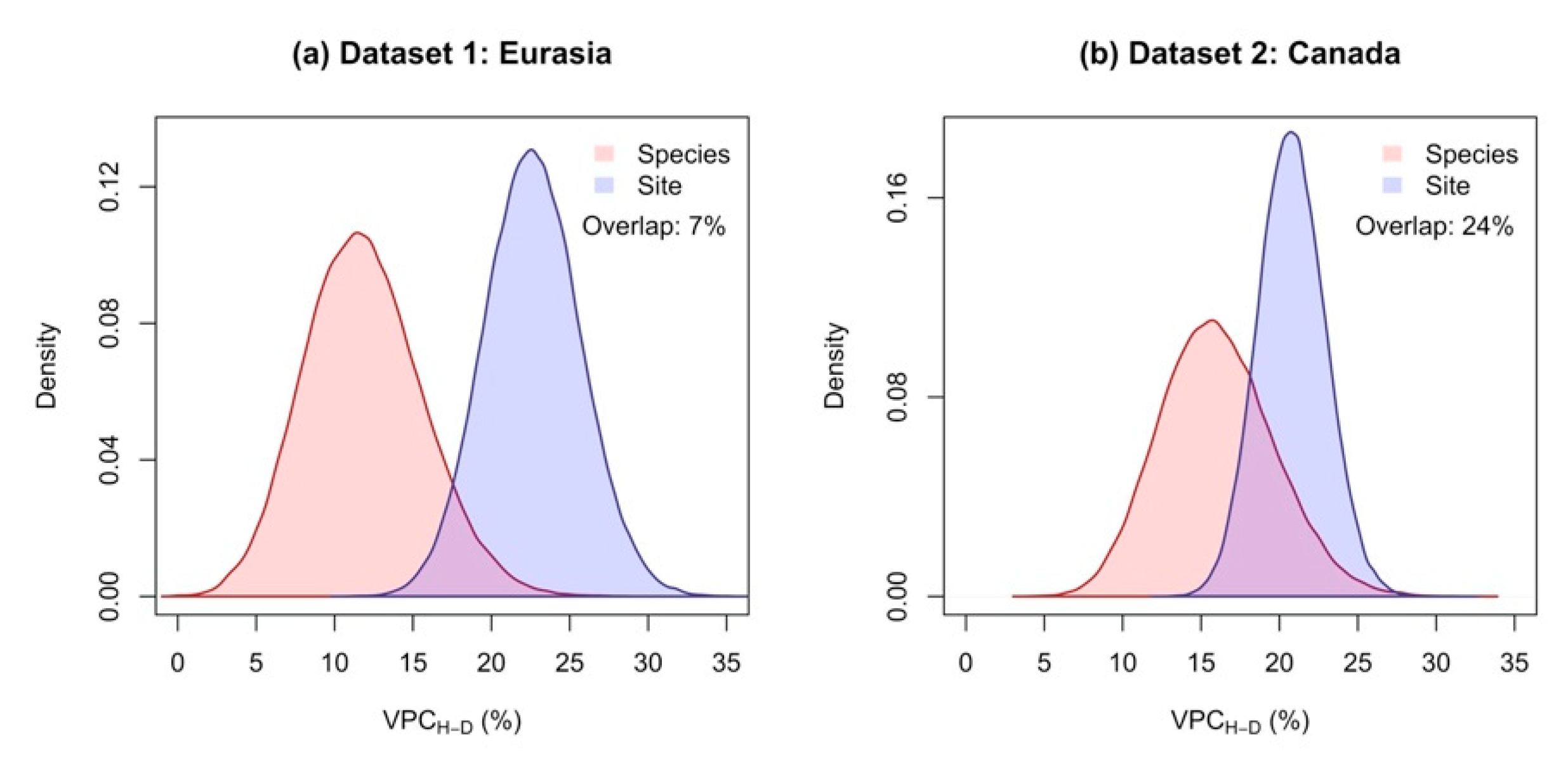
It is well known that including H in allometric models improves AGB prediction, because, for a tree of given D, if H is higher, the AGB is expected to be larger. Hence, H-D ratio is an important driver of variance in allometric models [55]. Including H in allometric biomass models, the variance explained by site, decreased (Figure 3). This suggests that there may be a greater variability of H-D ratio between sites than between species. Using the H-D ratio instead of relative residual in Equation (4), this hypothesis (i.e., H-D ratio varies more between sites than between species) was tested. The distributions of VPC for H-D ratio in Figure 5 confirm that the proportion of variance explained by site (Dataset 1: VPCH-D = 22.68%, SE = 3.75%; Dataset 2: VPCH-D = 20.77%, SE = 2.12%) was greater than that explained by species (Dataset 1: VPCH-D = 11.96%, SE = 3.05%; Dataset 2: VPCH-D = 16.17%, SE = 3.60%), for both datasets. Therefore, these results validate the assumption that, the reason for the reduction in site dependency of allometric models when H is included as a predictor, is related to the fact that H-D ratio varies more between sites than between species.
5. Conclusions
The key conclusions of the study are as follows: (1) Allometric biomass models were more species-specific than they were site-specific, the variance proportion explained by species (42.56%–47.54%) being larger than that explained by site (8.27%–20.08%); (2) including height in allometric biomass models (using D and H to predict AGB, instead of using D alone to predict AGB) helped reduce the dependency on site; (3) using the dendrogram to assess differences between species (regarding their biomass allometry) was practical and informative; (4) the lower proportion of variance explained by site within Dataset 2 (compared to Dataset 1), suggests that the negative consequences on prediction accuracy in transferring a species-specific allometric model from one site to another within Canada, are less severe compared to the transfers within Eurasia; (5) a large proportion of variance, caused by differences between species, indicates that a species-specific allometric biomass model should not be transferred to another species without appropriate model calibration, because that may induce large prediction bias.
Funding
This work was supported by a grant of the Romanian National Authority for Scientific Research and Innovation, CCCDI—UEFISCDI, project number ERANET-FACCE ERAGAS—FORCLIMIT (82/2017), within PNCDI II.
Acknowledgments
I am deeply grateful to all those who contributed to the data collection and to the authors who made these datasets available.
Conflicts of Interest
The author declares no conflict of interest.
References
- Chave, J.; Andalo, A.C.; Brown, A.S.; Cairns, A.M.A.; Chambers, J.Q.; Eamus, A.D.; Foïster, A.H.; Fromard, A.F.; Higuchi, N.; Kira, A.T.; et al. Tree allometry and improved estimation of carbon stocks and balance in tropical forests. Oecologia 2005, 145, 87–99. [Google Scholar] [CrossRef] [PubMed]
- Chave, J.; Réjou-Méchain, M.; Búrquez, A.; Chidumayo, E.; Colgan, M.S.; Delitti, W.B.C.; Duque, A.; Eid, T.; Fearnside, P.M.; Goodman, R.C.; et al. Improved allometric models to estimate the aboveground biomass of tropical trees. Glob. Chang. Biol. 2014, 20, 3177–3190. [Google Scholar] [CrossRef] [PubMed]
- Picard, N.; Saint-André, L.; Henry, M. Manual for Building Tree Volume and Biomass Allometric Equations: From Field Measurement to Prediction; FAO: Rome, Italy; CIRAD: Montpellier, France, 2012. [Google Scholar]
- Huxley, S.J. Problems of Relative Growth, 1st ed.; The Dial Press: New York, NY, USA, 1932. [Google Scholar]
- West, G.B.; Brown, J.H.; Enquist, B.J. A General Model for the Origin of Allometric Scaling Laws in Biology. Science 1997, 276, 122–126. [Google Scholar] [CrossRef] [PubMed]
- Enquist, B.J.; West, G.B.; Charnov, E.L.; Brown, J.H. Allometric scaling of production and life-history variation in vascular plants. Nature 1999, 401, 907–911. [Google Scholar] [CrossRef]
- Pretzsch, H. Species-specific allometric scaling under self-thinning: Evidence from long-term plots in forest stands. Oecologia 2006, 146, 572–583. [Google Scholar] [CrossRef] [PubMed]
- Zianis, D.; Radoglou, K. Comparison between empirical and theoretical biomass allometric models and statistical implications for stem volume predictions. Forestry 2006, 79, 477–487. [Google Scholar] [CrossRef] [Green Version]
- Wang, C. Biomass allometric equations for 10 co-occurring tree species in Chinese temperate forests. For. Ecol. Manag. 2006, 222, 9–16. [Google Scholar] [CrossRef]
- Ducey, M.J. Evergreenness and wood density predict height–diameter scaling in trees of the northeastern United States. For. Ecol. Manag. 2012, 279, 21–26. [Google Scholar] [CrossRef]
- Montagu, K.D.; Düttmer, K.; Barton, C.V.M.; Cowie, A.L. Developing general allometric relationships for regional estimates of carbon sequestration—an example using Eucalyptus pilularis from seven contrasting sites. For. Ecol. Manag. 2005, 204, 115–129. [Google Scholar] [CrossRef]
- Segura, V.; Cilas, C.; Costes, E. Dissecting apple tree architecture into genetic, ontogenetic and environmental effects: Mixed linear modelling of repeated spatial and temporal measures. New Phytol. 2008, 178, 302–314. [Google Scholar] [CrossRef]
- Fukatsu, E.; Nakada, R. The timing of latewood formation determines the genetic variation of wood density in Larix kaempferi. Trees 2018, 32, 1233–1245. [Google Scholar] [CrossRef]
- Barthélémy, D.; Caraglio, Y. Plant Architecture: A Dynamic, Multilevel and Comprehensive Approach to Plant Form, Structure and Ontogeny. Ann. Bot. 2007, 99, 375–407. [Google Scholar] [CrossRef] [PubMed] [Green Version]
- Urban, J.; Holušová, K.; Menšík, L.; Čermák, J.; Kantor, P. Tree allometry of Douglas fir and Norway spruce on a nutrient-poor and a nutrient-rich site. Trees 2013, 27, 97–110. [Google Scholar] [CrossRef]
- Archibald, S.; Bond, W.J. Growing tall vs. growing wide: Tree architecture and allometry of Acacia karroo in forest, savanna, and arid environments. Oikos 2003, 102, 3–14. [Google Scholar] [CrossRef]
- Dutcă, I.; Negruţiu, F.; Ioraş, F.; Maher, K.; Blujdea, V.N.B.; Ciuvăţ, L.A.; Negrutiu, F.; Ioras, F.; Maher, K.; Blujdea, V.N.B.; et al. The influence of age, location and soil conditions on the allometry of young Norway spruce ( Picea abies L. Karst.) trees. Not. Bot. Horti Agrobot. Cluj-Napoca 2014, 42, 579–582. [Google Scholar] [CrossRef]
- Poorter, H.; Niklas, K.J.; Reich, P.B.; Oleksyn, J.; Poot, P.; Mommer, L. Biomass allocation to leaves, stems and roots: Meta-analyses of interspecific variation and environmental control. New Phytol. 2012, 193, 30–50. [Google Scholar] [CrossRef]
- Delucia, E.H.; Maherali, H.; Carey, E.V. Climate-driven changes in biomass allocation in pines. Glob. Chang. Biol. 2000, 6, 587–593. [Google Scholar] [CrossRef]
- António, N.; Tomé, M.; Tomé, J.; Soares, P.; Fontes, L. Effect of tree, stand, and site variables on the allometry of Eucalyptus globulus tree biomass. Can. J. For. Res. 2007, 37, 895–906. [Google Scholar] [CrossRef]
- Yang, B.; Xue, W.; Yu, S.; Zhou, J.; Zhang, W. Effects of Stand Age on Biomass Allocation and Allometry of Quercus Acutissima in the Central Loess Plateau of China. Forests 2019, 10, 41. [Google Scholar] [CrossRef]
- Lines, E.R.; Zavala, M.A.; Purves, D.W.; Coomes, D.A. Predictable changes in aboveground allometry of trees along gradients of temperature, aridity and competition. Glob. Ecol. Biogeogr. 2012, 21, 1017–1028. [Google Scholar] [CrossRef]
- Naidu, S.L.; DeLucia, E.H.; Thomas, R.B. Contrasting patterns of biomass allocation in dominant and suppressed loblolly pine. Can. J. For. Res. 1998, 28, 1116–1124. [Google Scholar] [CrossRef]
- Dutcă, I.; Mather, R.; Ioraş, F. Tree biomass allometry during the early growth of Norway spruce (Picea abies) varies between pure stands and mixtures with European beech (Fagus sylvatica). Can. J. For. Res. 2018, 48, 77–84. [Google Scholar] [CrossRef]
- Messier, C.; Mitchell, A.K. Effects of thinning in a 43-year-old Douglas-fir stand on above- and below-ground biomass allocation and leaf structure of understory Gaultheria shallon. For. Ecol. Manag. 1994, 68, 263–271. [Google Scholar] [CrossRef]
- Fayolle, A.; Doucet, J.-L.; Gillet, J.-F.; Bourland, N.; Lejeune, P. Tree allometry in Central Africa: Testing the validity of pantropical multi-species allometric equations for estimating biomass and carbon stocks. For. Ecol. Manag. 2013, 305, 29–37. [Google Scholar] [CrossRef]
- Ngomanda, A.; Engone Obiang, N.L.; Lebamba, J.; Moundounga Mavouroulou, Q.; Gomat, H.; Mankou, G.S.; Loumeto, J.; Midoko Iponga, D.; Kossi Ditsouga, F.; Zinga Koumba, R.; et al. Site-specific versus pantropical allometric equations: Which option to estimate the biomass of a moist central African forest? For. Ecol. Manag. 2014, 312, 1–9. [Google Scholar] [CrossRef]
- Xiang, W.; Zhou, J.; Ouyang, S.; Zhang, S.; Lei, P.; Li, J.; Deng, X.; Fang, X.; Forrester, D.I. Species-specific and general allometric equations for estimating tree biomass components of subtropical forests in southern China. Eur. J. For. Res. 2016, 135, 963–979. [Google Scholar] [CrossRef]
- Paul, K.I.; Roxburgh, S.H.; Ritson, P.; Brooksbank, K.; England, J.R.; Larmour, J.S.; John Raison, R.; Peck, A.; Wildy, D.T.; Sudmeyer, R.A.; et al. Testing allometric equations for prediction of above-ground biomass of mallee eucalypts in southern Australia. For. Ecol. Manag. 2013, 310, 1005–1015. [Google Scholar] [CrossRef]
- Paul, K.I.; Roxburgh, S.H.; Chave, J.; England, J.R.; Zerihun, A.; Specht, A.; Lewis, T.; Bennett, L.T.; Baker, T.G.; Adams, M.A.; et al. Testing the generality of above-ground biomass allometry across plant functional types at the continent scale. Glob. Chang. Biol. 2016, 22, 2106–2124. [Google Scholar] [CrossRef]
- Ishihara, M.I.; Utsugi, H.; Tanouchi, H.; Aiba, M.; Kurokawa, H.; Onoda, Y.; Nagano, M.; Umehara, T.; Ando, M.; Miyata, R.; et al. Efficacy of generic allometric equations for estimating biomass: A test in Japanese natural forests. Ecol. Appl. 2015, 25, 1433–1446. [Google Scholar] [CrossRef]
- Vieilledent, G.; Vaudry, R.; Andriamanohisoa, S.F.D.; Rakotonarivo, O.S.; Randrianasolo, H.Z.; Razafindrabe, H.N.; Bidaud Rakotoarivony, C.; Ebeling, J.; Rasamoelina, A.M.; Rakotoarivony, C.B.; et al. A universal approach to estimate biomass and carbon stock in tropical forests using generic allometric models. Ecol. Appl. 2012, 22, 572–583. [Google Scholar] [CrossRef]
- Rutishauser, E.; Noor′an, F.; Laumonier, Y.; Halperin, J.; Hergoualc’h, K.; Verchot, L. Generic allometric models including height best estimate forest biomass and carbon stocks in Indonesia. For. Ecol. Manag. 2013, 307, 219–225. [Google Scholar] [CrossRef]
- Schepaschenko, D.; Shvidenko, A.; Usoltsev, V.; Lakyda, P.; Luo, Y.; Vasylyshyn, R.; Lakyda, I.; Myklush, Y.; See, L.; McCallum, I.; et al. A dataset of forest biomass structure for Eurasia. Sci. Data 2017, 4, 170070. [Google Scholar] [CrossRef] [PubMed]
- Ung, C.H.; Bernier, P.; Guo, X.J. Canadian national biomass equations: New parameter estimates that include British Columbia data. Can. J. For. Res. 2008, 38, 1123–1132. [Google Scholar] [CrossRef]
- Ung, C.H.; Lambert, M.C.; Raulier, F.; Guo, X.J.; Bernier, P.Y. Biomass of trees sampled across Canada as part of the Energy from the Forest Biomass (ENFOR) Program 2017. Available online: https://doi.org/10.23687/fbad665e-8ac9-4635-9f84-e4fd53a6253c (accessed on 21 December 2018).
- Clarke, P. When can group level clustering be ignored? Multilevel models versus single-level models with sparse data. J. Epidemiol. Community Health 2008, 62, 752–758. [Google Scholar] [CrossRef] [PubMed]
- Goldstein, H.; Browne, W.; Rasbash, J. Partitioning Variation in Multilevel Models. Underst. Stat. 2002, 1, 223–231. [Google Scholar] [CrossRef]
- Kish, L. Survey Sampling; John Wiley & Sons: New York, NY, USA, 1965. [Google Scholar]
- Enquist, B.J.; Niklas, K.J. Invariant scaling relations across tree-dominated communities. Nature 2001, 410, 655–660. [Google Scholar] [CrossRef]
- Baskerville, G.L. Use of Logarithmic Regression in the Estimation of Plant Biomass. Can. J. For. Res. 1972, 2, 49–53. [Google Scholar] [CrossRef]
- Sprugel, D.G. Correcting for Bias in Log-Transformed Allometric Equations. Ecology 1983, 64, 209–210. [Google Scholar] [CrossRef]
- Bates, D.; Mächler, M.; Bolker, B.; Walker, S. Fitting Linear Mixed-Effects Models using lme4. J. Stat. Softw. 2015, 67, 1–48. [Google Scholar] [CrossRef]
- R Core Team. R: A Language and Environment for Statistical Computing; R Foundation for Statistical Computing: Vienna, Austria, 2017. [Google Scholar]
- Murtagh, F.; Legendre, P. Ward′s Hierarchical Agglomerative Clustering Method: Which Algorithms Implement Ward’s Criterion? J. Classif. 2014, 31, 274–295. [Google Scholar] [CrossRef]
- Hollister, J.; Shah, T. Elevatr: Access Elevation Data from Various APIs; US EPA Office of Research and Development: Washington, DC, USA, 2017.
- Pastore, M. Overlapping: A R package for Estimating Overlapping in Empirical Distributions. J. Open Source Softw. 2018, 3, 1–4. [Google Scholar] [CrossRef]
- Sarkar, D. Lattice: Multivariate Data Visualization with R, 1st ed.; Springer: Seattle, WA, USA, 2008. [Google Scholar]
- Galili, T. dendextend: An R package for visualizing, adjusting and comparing trees of hierarchical clustering. Bioinformatics 2015, 31, 3718–3720. [Google Scholar] [CrossRef] [PubMed]
- Hijmans, R.J. Raster: Geographic Data Analysis and Modeling 2019. R package version 3.0-2. Available online: https://CRAN.R-project.org/package=raster (accessed on 10 September 2019).
- Iida, Y.; Poorter, L.; Sterck, F.J.; Kassim, A.R.; Kubo, T.; Potts, M.D.; Kohyama, T.S. Wood density explains architectural differentiation across 145 co-occurring tropical tree species. Funct. Ecol. 2012, 26, 274–282. [Google Scholar] [CrossRef]
- Henry, M.; Besnard, A.; Asante, W.A.; Eshun, J.; Adu-Bredu, S.; Valentini, R.; Bernoux, M.; Saint-André, L. Wood density, phytomass variations within and among trees, and allometric equations in a tropical rainforest of Africa. For. Ecol. Manag. 2010, 260, 1375–1388. [Google Scholar] [CrossRef]
- Hijmans, R.J.; Cameron, S.E.; Parra, J.L.; Jones, P.G.; Jarvis, A. Very high resolution interpolated climate surfaces for global land areas. Int. J. Climatol. 2005, 25, 1965–1978. [Google Scholar] [CrossRef]
- Swenson, N.G.; Enquist, B.J. Ecological and evolutionary determinants of a key plant functional trait: Wood density and its community-wide variation across latitude and elevation. Am. J. Bot. 2007, 94, 451–459. [Google Scholar] [CrossRef]
- Feldpausch, T.R.; Lloyd, J.; Lewis, S.L.; Brienen, R.J.W.; Gloor, M.; Monteagudo Mendoza, A.; Lopez-Gonzalez, G.; Banin, L.; Abu Salim, K.; Affum-Baffoe, K.; et al. Tree height integrated into pantropical forest biomass estimates. Biogeosciences 2012, 9, 3381–3403. [Google Scholar] [CrossRef] [Green Version]
Figure 1.
The number of trees per species (a), and the number of trees per site (b) presented in base 10 log scale.
Figure 1.
The number of trees per species (a), and the number of trees per site (b) presented in base 10 log scale.
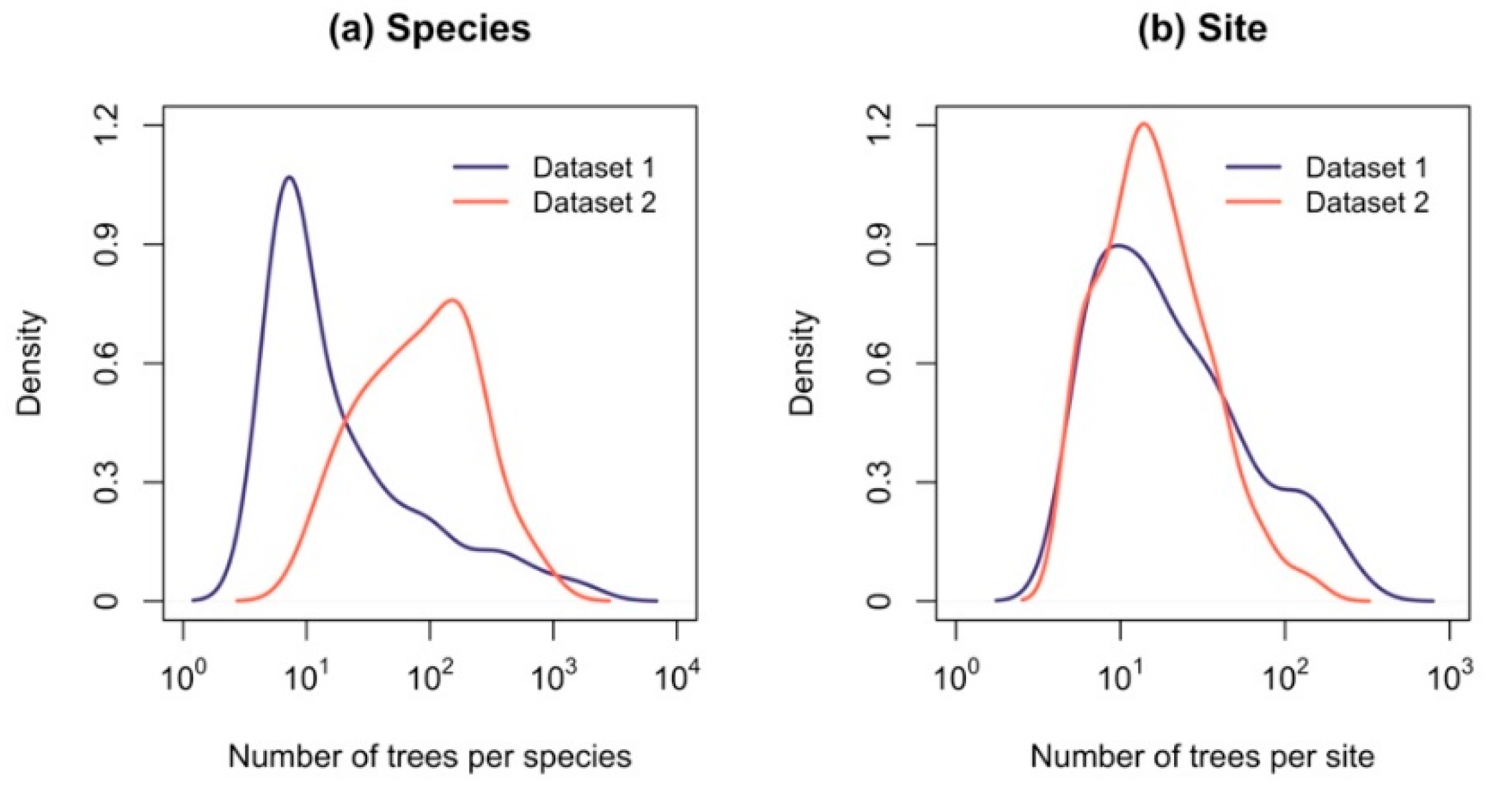
Figure 2.
The Variance Partition Coefficient (VPC) density, for Dataset 1 (a) and Dataset 2 (b). Note: The density curves are based on VPC values resulted from bootstrap analysis; the ‘overlap’ shows the percentage of the overlapping regions of the two distributions.
Figure 2.
The Variance Partition Coefficient (VPC) density, for Dataset 1 (a) and Dataset 2 (b). Note: The density curves are based on VPC values resulted from bootstrap analysis; the ‘overlap’ shows the percentage of the overlapping regions of the two distributions.
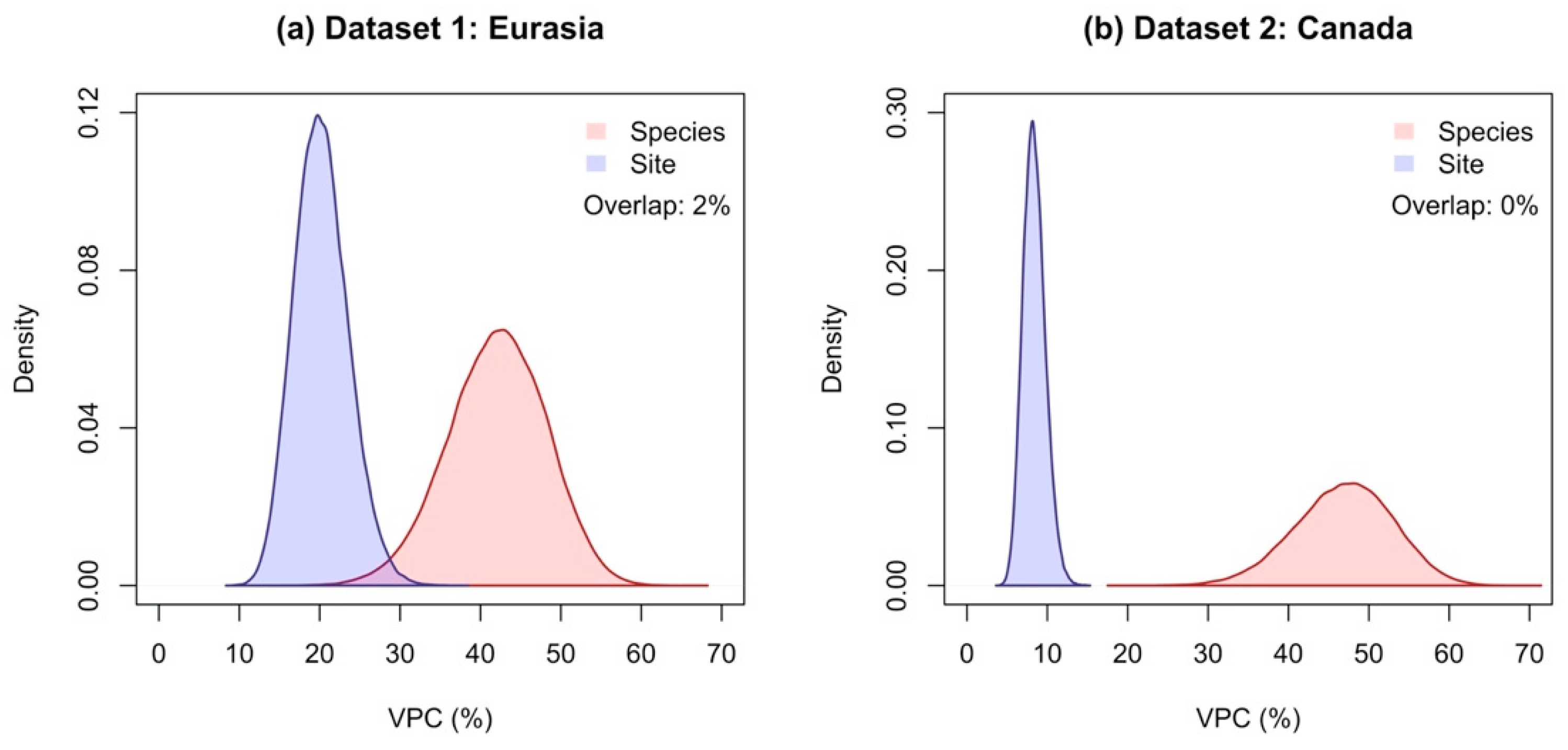
Figure 3.
The Variance Partition Coefficient (VPC) density for models based on D only (AGB = f(D)) and for models based on both D and H (AGB = f(D, H)). Note: The density curves are based on VPC values resulted from bootstrap analysis; the ‘overlap’ shows the percentage of the overlapping regions of the two distributions.

Figure 4.
The dendrograms showing the grouping of species by their allometry, for Dataset 1 and Dataset 2. Note: (1) The γk values (Equation (4)) are presented in parenthesis for each species (γk was centred to zero by subtracting the mean μ from each γk value) and the sample size for each species. (2) In different colours are the species that were grouped by cutting the dendrogram at a distance of 1.0 (vertical dashed red line).
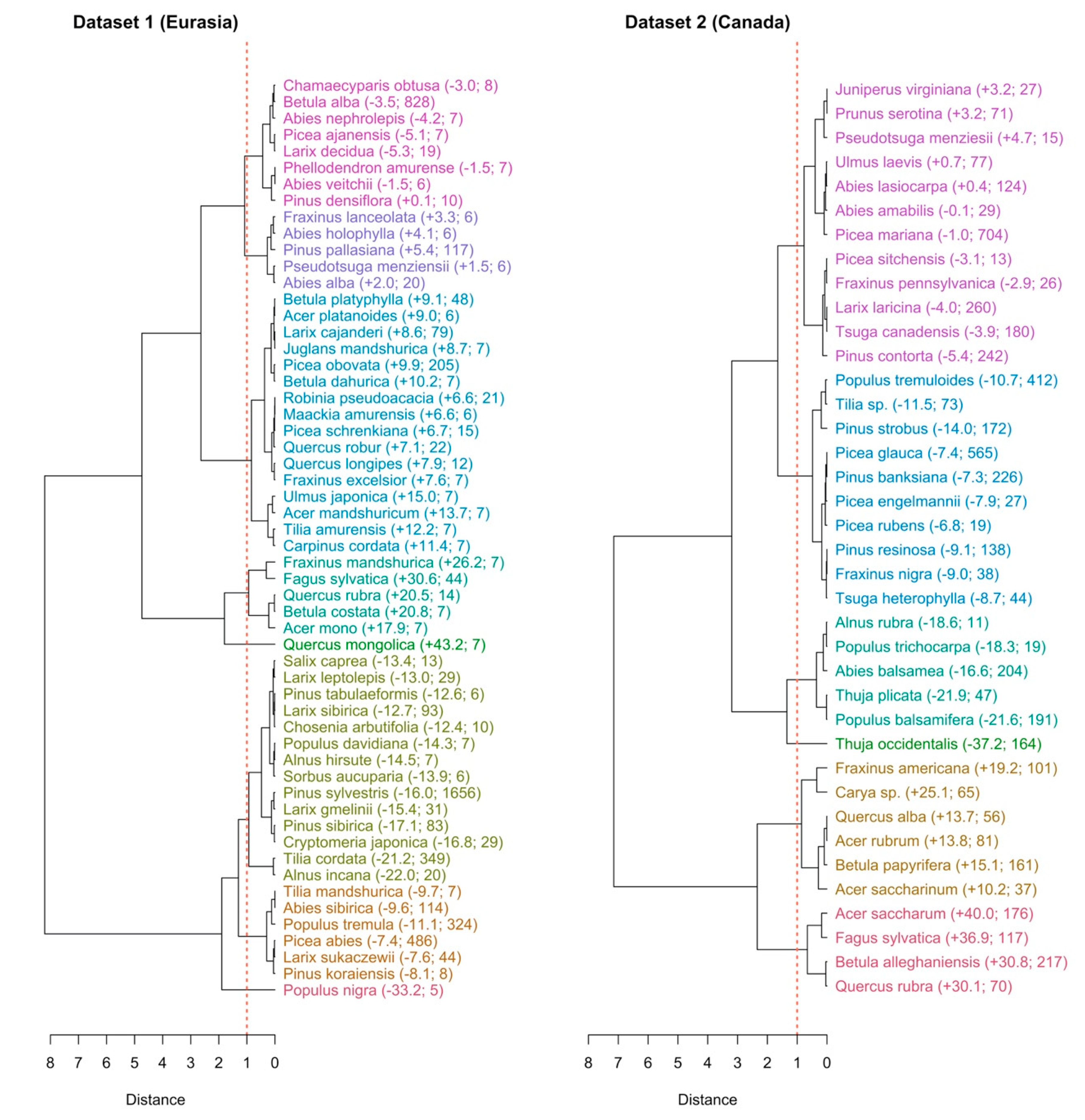
Figure 5.
The VPCH-D, showing the proportion of variance caused by differences between species and differences between sites in the variability of H-D ratio (ratio between height and diameter at breast height).
Figure 5.
The VPCH-D, showing the proportion of variance caused by differences between species and differences between sites in the variability of H-D ratio (ratio between height and diameter at breast height).

Table 1.
The characteristics of analyzed datasets.
| Characteristic | Dataset 1 | Dataset 2 |
|---|---|---|
| Region | Europe and Asia | Canada |
| Sample size | 4921 | 5199 |
| D range (cm) | 5.0–72.9 | 5.0–74.3 |
| H range (m) | 3.1–42.8 | 2.5–40.8 |
| AGB range (kg) | 2.2–4291.3 | 2.2–2951.4 |
| Number of tree species | 56 | 38 |
| Number of trees per species (range) | 5–1656 | 11–704 |
| Number of sites | 133 | 237 |
| Number of trees per site (range) | 5–278 | 5–164 |
| References | [34] | [35,36] |
© 2019 by the author. Licensee MDPI, Basel, Switzerland. This article is an open access article distributed under the terms and conditions of the Creative Commons Attribution (CC BY) license (http://creativecommons.org/licenses/by/4.0/).
Share and Cite
MDPI and ACS Style
Dutcă, I. The Variation Driven by Differences between Species and between Sites in Allometric Biomass Models. Forests 2019, 10, 976. https://doi.org/10.3390/f10110976
AMA Style
Dutcă I. The Variation Driven by Differences between Species and between Sites in Allometric Biomass Models. Forests. 2019; 10(11):976. https://doi.org/10.3390/f10110976
Chicago/Turabian StyleDutcă, Ioan. 2019. "The Variation Driven by Differences between Species and between Sites in Allometric Biomass Models" Forests 10, no. 11: 976. https://doi.org/10.3390/f10110976
Note that from the first issue of 2016, this journal uses article numbers instead of page numbers. See further details here.