1. Introduction
Wildland firefighting requires that managers make decisions to manage risk within complex decision environments that hold many uncertainties. Some of the challenges for managers include determining when and where to place firefighting activities, what those activities should be, how many and what type of firefighting resources are available and which are the best fit for the fire management tasks that must be completed [
1,
2,
3]. Managers must make these assignments while balancing a variety of risks including loss of life to both firefighters and the public; loss of infrastructure such as buildings and power lines; loss of natural resources such as habitat for wildlife, timber, and recreation areas; and damage that threatens water quality [
1,
2,
3]. These complex suppression decisions need to be adapted dynamically over time. The outcome of fire suppression actions hinge on future fire behavior, which is highly dependent upon weather (e.g., [
4,
5,
6,
7,
8,
9,
10]). For example, a fireline built to withstand a low intensity fire [
10] may contain the fire as long as the fire is still low intensity when it encounters the fireline. If the wind picks up and the fireline intensity increases, the fireline may do little to reduce fire growth. In addition, while firefighting tasks may be completed with the goal of stopping fire spread, other tasks may be undertaken with the goal of slowing a fire or decreasing its intensity [
1,
11]. As a fire evolves, management actions must consider new developments and changes in fire behavior. For example, many large fires include contingency line which is built in case primary line fails [
12]. While empirical research regarding fireline effectiveness is limited [
13,
14], fire managers do consider expected and worst-case fire behavior when considering where suppression actions are most likely to successfully control the fire [
13]. Thus, for a model to adequately account for suppression-fire interactions, such activities must be modeled over time and interact dynamically with fire behavior.
Models have been built to address some of these important considerations. For example, Fried and Fried [
15] developed a simulation algorithm to explicitly account for the interaction between fireline production and fire growth, i.e., that fire growth is hampered by fireline production. Their model has been used in operational programs such as CFES2, a fire suppression budgeting model for California [
16]. This model assumes fireline is produced along the edge of the fire, reducing further growth as it is produced. While the model developed by Fried and Fried [
15] does account for the interaction between fireline production and fire growth, it is typically implemented in a quasi-spatial manner, where the fire is assumed to take the shape of an ellipse and spreads from a single ignition point on a homogeneous landscape [
16].
Other models have been developed that select containment tactics. For example, HomChaudhuri et al. [
17] developed a genetic algorithm for placing wildfire suppression on a landscape, using their model to determine the optimal starting and ending points of the suppression resources along with the parameters of the parametric equation that determines the suppression resources’ path. While the fitness of the solution is evaluated under uncertain weather behavior and within the fitness evaluation process the suppression actions may interact with fire to change final fire behavior, only one solution is provided; the solution does not consider that recourse decisions may vary as the fire evolves. Stochastic simulation methods have also been developed to configure and evaluate spatially explicit tactical suppression decisions. Hu and Ntaimo [
18] simulated fireline construction for a single fire using stochastic line production parameters. They developed three algorithms for their simulation to model direct attack, parallel attack, and indirect attack. Like HomChaudhuri et al. [
17], their model provides a single solution that does not consider multiple future scenarios and possible recourse actions. Alexandridis et al. [
19] developed a cellular stochastic model to simulate the effects of air tanker attack. A Poisson distribution is used to determine if an air attack will take place on a cell and the probability that fire will be extinguished in a cell after an air attack takes place. This model examines the effectiveness of air tanker suppression actions, but assumes a predefined set of suppression actions and does not examine how to plan or design such actions. Mees and Strauss [
20] incorporated random effects into a mathematical programming model using probabilistic fireline production rates. This model maximizes expected utility, defined as the sum of the probabilities that different sections of line will hold weighted by the relative importance of the sections and subject to resource availability constraints. The suppression actions are predefined to be specific sections of line; the decisions made by the model are which resources to place at each fireline segment. Spatial relationships between the fireline segments are not modeled. All these previous studies model suppression decisions such that they cannot interact dynamically with fire or they cannot be updated over time, thus, they may be sub-optimal decisions. Likewise, none of the previous studies integrate explicitly spatial and temporal stochastic fire behavior with explicitly spatial and temporal endogenous suppression decisions that account for crew movement, crew safety, line production, and line quality. Many other operations research projects have examined optimizing resource assignments but they are not as relevant to our research as the papers we discuss in detail above; we refer readers interested in further exploring this topic to [
11,
21,
22].
A stochastic mixed integer programming (SMIP) model [
23] to optimize suppression decisions that dynamically interact with uncertain fire behavior on a single fire was developed by Belval et al. [
24]. That model provided a framework for selecting suppression activities that alter resultant fire behavior; first stage decisions were the initial suppression actions and second stage decisions were follow up suppression actions. It included explicit nonanticipativity constraints to ensure suppression decisions that account for uncertainty in weather forecasts and recourse decisions allowed the model to create optimal suppression decisions for each weather scenario. In addition, that model incorporated flexible decision points, which allowed a variety of management styles to be represented. The model presented in Belval et al. [
24] integrates suppression decisions using “suppression node placements” which model the timing and placement of suppression actions on the landscape. However, two of the main assumptions underlying the suppression node placement model of suppression are simplistic. First, these suppression actions are modeled assuming all cells on the landscape are associated with a single, constant, fireline production rate, but actual production rates may vary depending on factors such as fire intensities, topography, and fuel type [
1,
25]. Second, suppression placements themselves are oversimplified. For example, the constraints did not explicitly require fire suppression resource movement to be continuous even though crews, engines, and bulldozers must travel in a continuous fashion (i.e., these resources cannot fly or apparate and travel time between suppression locations are not negligible). While the solutions produced by the model did tend to be continuous, simply because continuous line was required to contain the fire, the model did not include constraints requiring any type of continuity, particularly regarding temporal continuity. To model suppression more realistically, the spatial and temporal restrictions on the fire crews must be modeled with such additional details included. In addition, the suppression nodes do not consider crew safety or line quality, which are integral aspects of fire suppression.
In this paper, a set of constraints is developed to model firefighting activities and control lines that allow for more realistic simulation of crew tactics and safety concerns which are integrated with the previously developed SMIP fire spread model [
24]. These constraints are specifically designed for ground-based tactics (i.e., crew or engine activities), particularly targeting initial line construction; aerial resources and “mop-up” (i.e., reducing the probability of fire spread or smoke by extinguishing residual burning material along a previously built control line) are not represented in this model. Based on our knowledge, this is the first time an SMIP model is developed to explicitly address fireline quality, firefighter travel path connectivity, firefighter safety and their interaction with uncertain fire behaviors to provide optimal suppression suggestions for fireline construction. Our results demonstrate the value of modeling additional details of fire suppression using this SMIP framework. The test cases are small to allow this paper to focus on the development and details of the control constraints; future work to expand scenarios, add other objectives and constraints, and gather necessary data is addressed in the discussion.
3. Results
The results from model runs of the standard safety margin test case, the reduced decision space test case, and the higher safety margin test case are shown in
Figure 4,
Figure 5 and
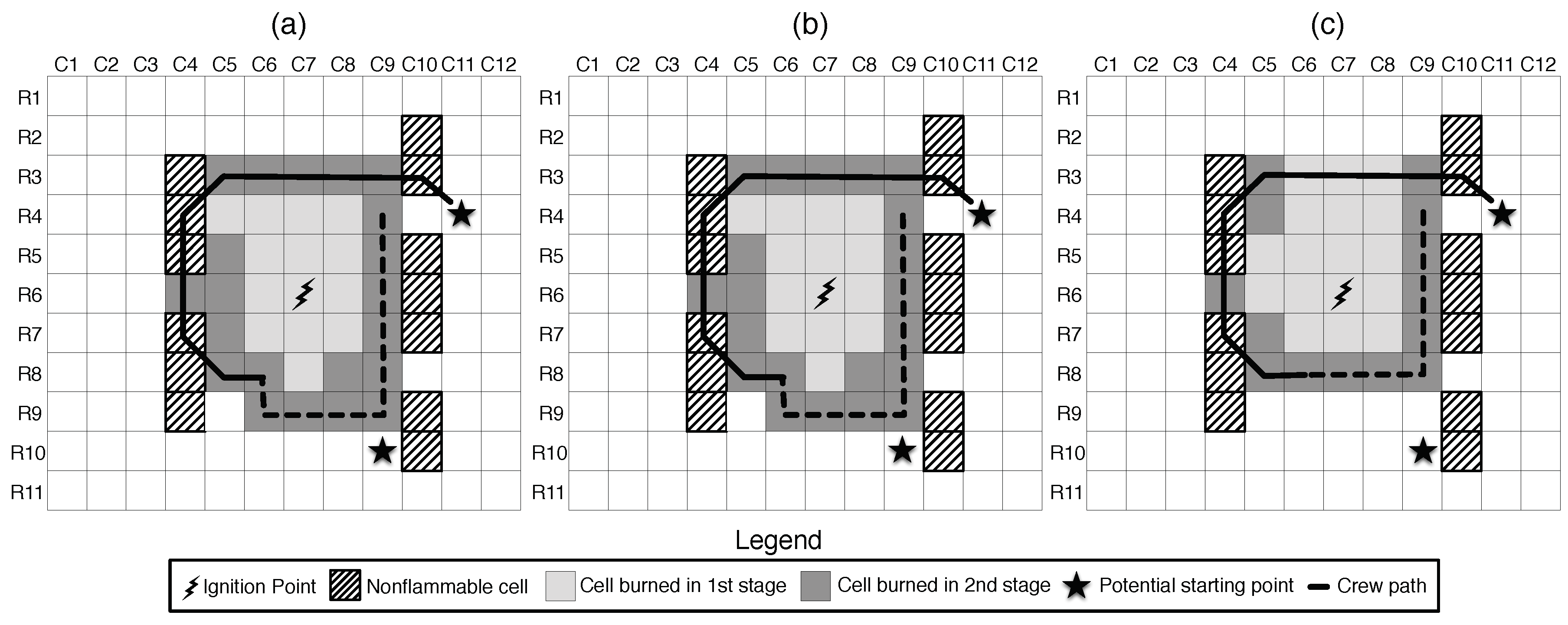
Figure 6, respectively. Columns a, b, and c in these figures correspond to the results from scenarios a, b, and c, respectively. Each of these figures shows the stage in which fire arrived at each node, the possible access points, the ignition point, non-flammable nodes, and the optimal crew path by stage as determined by the model.
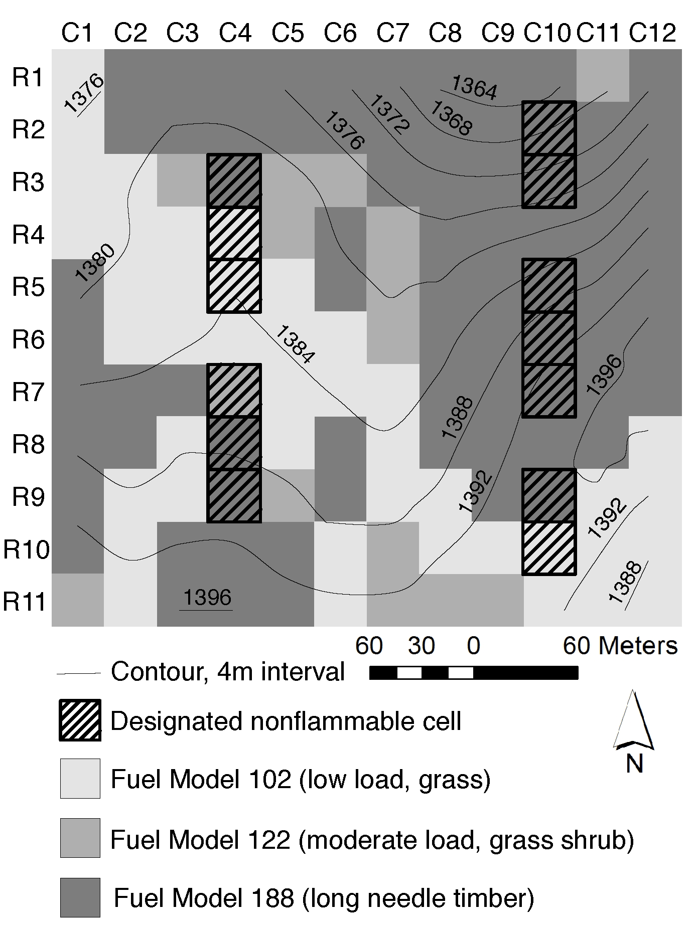
In all three test cases the crews travel quickly through the non-flammable cells on the western edge of the ignition (C4, R4-8) and spend the majority of their time working at the nodes on the north, east and south edges of the fire. For each test case, the suppression actions are the same for the first 30 min in all scenarios, as required by first stage nonanticipativity constraints. After 30 minutes, the first and second scenarios still have identical suppression actions as required by second stage nonanticipativity constraints while the suppression actions in the third scenario differ.
In all of the scenarios for the standard safety margin and higher safety margin test cases (
Figure 4 and
Figure 6) the crews access but do not put any work into cell (C9, R6); they only travel through it. This is because the model assumes that putting suppression in a cell does not keep it from burning; rather, it prevents the cell from spreading fire to other cells. Thus, in all three scenarios, cells (C9, R7-9) and (C9, R3-5) are suppressed to keep fire from spreading into (C10, R8) and (C10, R4) respectively, but putting suppression effort in (C9, R6) would have no effect on the number of cells burned.
The results of the reduced decision space test case (
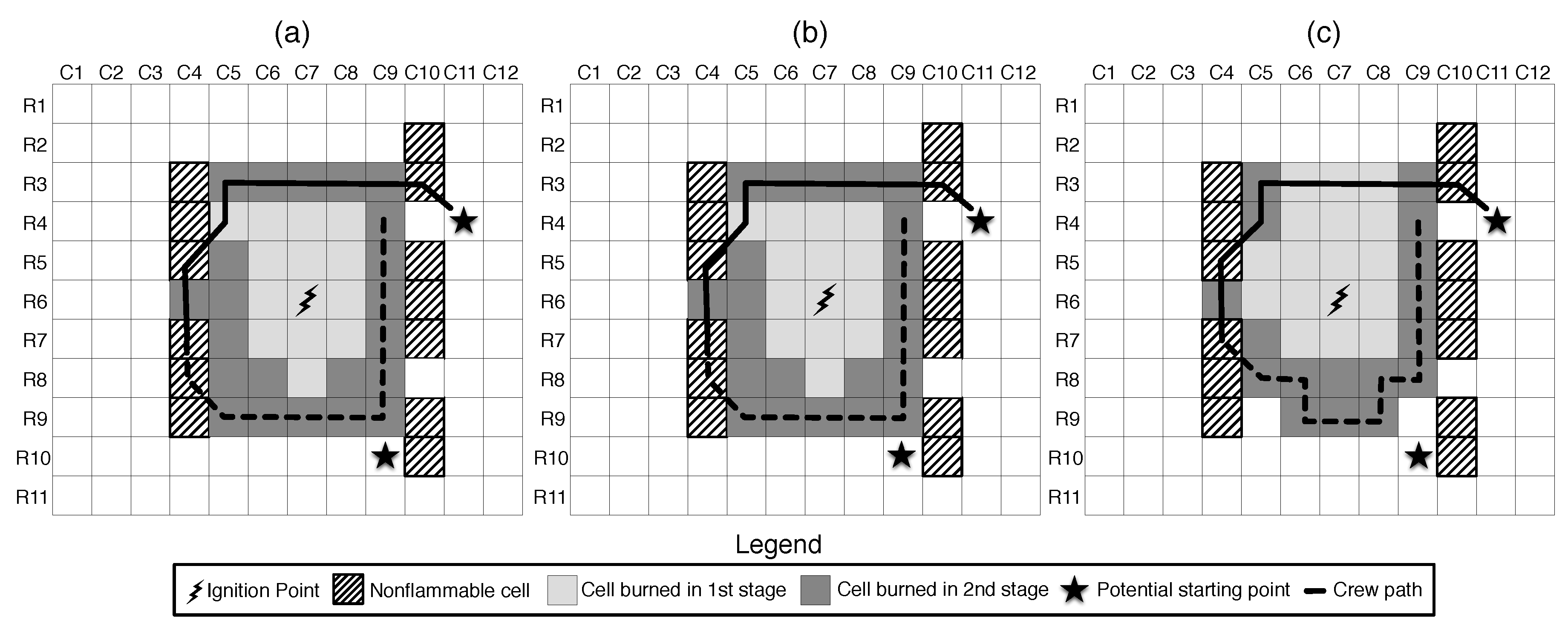
Figure 5) compared with the results of the standard safety margin test case demonstrate some effects of using a reduced decision space. Because the suppression lines have been pre-identified, the crew path is more straightforward (i.e., straight lines rather than winding around cells with earlier fire arrival times). For example, the suppression path along the south flank of the fire runs straight along row 9 in the reduced decision test case, while in the standard safety margin case the path goes from (R8, C8) to (R9, C8). In addition, the suppression path is forced to follow the non-flammable cells more closely, resulting in less work for the crew, although the travel distance is slightly longer. For example, in
Figure 4, the optimal solution places suppression activities in three cells (C9, R3-5) to keep one cell from burning. Placing suppression effort in only two cells (C10, R4) and (C9, R3) instead would result in nearly the same fire footprint but with less effort from the crew. This is evident in the reduced decision space test case (
Figure 5). The crew travels an expected 3% further (18.3 meters), however, requires less work time to contain the fire. Only 2.67 extra cells are expected to burn (an 8% increase in expected burned area). The pre-identified paths such as those used in the reduced decision space test case may be appealing to managers as they create fire suppression plans and managers may decide the slightly larger expected burned area is worth the tradeoff of less suppression work along pre-identified control lines.
Because of the integer nature of the model and the specific test cases we chose, examples of binding completion times are few, i.e., there are no cells where the work completion time is exactly equal to the fire arrival time minus the safety buffer. However, there are numerous examples of cells that cannot have suppression placed in them due to work completion time and safety buffer requirements. For example, in the standard safety margin test case (
Figure 4), scenarios a and b, the model places suppression in cells (C5-6, R8), which prevents cell (C5, R9) from burning. However, the crew must then avoid cells (C7-8, R8) because they would not arrive at these cells before fire has arrived, which forces the crews to move around these cells, taking their path through (C6-8, R9). Because these actions occur in the second stage of the model, scenario c is not bound by nonanticipativity to produce the same crew actions as scenarios a and b, and because the fire arrives later at (C7-8, R8) in scenario c, the solution for scenario c is to place line in cells (C7-8, R8), reducing the burned area by four cells as compared with scenarios a and b. These differing crew paths also demonstrate another interesting aspect of the model: it can deliberately add slack into the work time in order to delay the completion of work such that the next node in a path is no longer bound by the nonanticipativity constraints. When the slack is removed from the work completion times, the crew can finish their work at cell (C6, R8) by 29 min. However, the model chose a work completion time of exactly 30 min. Although this difference of less than a minute may seem minor, the model chose to have the crew pause here to transition to the second decision stage, which is not constrained by the first stage nonanticipativity constraints. After 30 min has passed, the paths and work times of scenario c may differ from those of scenarios a and b, allowing the crew to save four extra cells in scenario c. In reality, the crews could certainly see if the fire had reached a cell before they got there, and it would not be difficult to decide whether or not to go around. The model is planning crew work ahead of time, and thus waits until the uncertainty is resolved to make a decision about where the crew will go in the second stage.
In our test cases we identified one specific example of suppression actions affecting fire behavior. In scenario c, for all test cases, fire arrives in cell (C5, R3) in the second stage. However, when the model is run with no suppression, fire arrives in cell (C5, R3) in the first stage. In the no suppression test case, fire spreads from cell (C6, R3) into (C5, R3). Because suppression is placed in (C6, R3) in each of the test cases with suppression, fire can no longer spread from (C6,R3) to (C5, R3), forcing fire along a slower spread path. This delays fire arrival time to (C5, R3) from the first stage to the second stage. Interestingly, it also increases the fireline intensity from 398 BTU (ft-s) to 423 BTU (ft-s). While this does not substantially affect the crew paths or work times in these test cases, modeling such interactions between fire and suppression may affect the feasibility of fire suppression tactics in other cases.
The only difference in parameters between the models used to produce
Figure 4 and
Figure 6 is a higher safety margin parameter was used for
Figure 6 (see
Table 4). The higher safety margin parameter results in some interesting differences between solutions. Because of the higher safety margin parameter, the crew can no longer make it out of cell (C6, R8) in time in scenarios a and b, thus the crew path changes such that the crew no longer travels or works in (C6, R8). Similarly, because the crew cannot be in cell (C6, R8) in scenarios a and b, the crew cannot arrive in time to suppress fire in cell (C7, R8) in scenario c. Therefore, the model delays the crew at cell (C4, R5) so that it can make decisions for subsequent suppression without being bound by the nonanticipativity constraints. Because we know from the results in the standard safety margin test case (
Figure 4) that the crew could have finished that work much sooner, we observe that there is enough slack in the work time and crew arrival time constraints to allow the model to delay at cell (C4, R5) even though the crew path would have allowed the delay to be as late as at (C4, R7); such solutions are alternative optima.
Finding an initial feasible solution for CPLEX can be challenging with this model. To get a feasible solution quickly, we first reduced the number of cells in which the crews could work, giving the crews only one option for a path around the fire. This reduced problem always solved within one minute of run time, providing us with an MIP start. When solving the full problem with the pre-identified MIP start, CPLEX typically found the optimal solution within ten minutes of run time. However, CPLEX often still reported a large MIP gap (anywhere from 30% to 70%) even after the optimal solution was initially found. For the results presented in this paper we allowed CPLEX to run until optimality was established. On a desktop computer with 32GB of RAM, it sometimes took days to reduce the MIP gap; in some cases (for results not presented in this paper) the gap could not be eliminated prior to the computer running out of memory.
4. Discussion
The suppression constraints presented in this paper incorporate detailed suppression considerations for ground-based firefighting resources combined with stochastic fire behavior to create a framework from which fire suppression decisions can be modeled. Spatial restrictions requiring continuous crew movements were enforced as were safety restrictions for crews. Fireline quality was modeled using control line capacity defined as the maximum fireline intensity at which the fireline will hold. The solutions to the model provide a map of the optimal path for each crew and determine the amount of work that needs to be done on each node. These constraints provide useful information to a manager.
In practice, a manager could pre-identify areas of the landscape that are of particular importance to protect; those areas could be heavily weighted in the objective function to encourage a solution that protects those areas. The solution presented by the model will provide a decision maker with a good sense for safe, feasible places to put fireline, even given variable future weather scenarios. If the prioritized areas remain unprotected by the solution the manager might re-examine why they are unprotected (i.e., not enough resources, the line will not hold in all scenarios, safety concerns). Then the solution may be adjusted by the manager to reflect any concerns that the model missed. Using this model or a similar one would provide a risk management-based process to help determine resource assignments. Additional research to investigate fire manager risk preferences and practices regarding risk management would be necessary. Current research indicates managers do explicitly consider expected and worst-case fire behavior [
13,
14], but very little work has been done to qualify, quantify or compare how this plays into the managers’ decision making process in practice.
This suppression model could be improved to better represent reality. For example, if fireline does not stop a fire, it may still slow the fire down. A delay could be incorporated when fire spreads across a fireline or retardant. In the results presented here, costs of line construction are not considered. However, explicit costs could be added; both the fixed cost associated with dispatching a crew to the fire and the variable costs of the work the crew produces could be added to the model. Some assumptions made to formulate our current constraints might also be relaxed. For example, one assumption integral to the spatial crew constraints is that each crew is only allowed at each node once. This model could be modified to include a second arrival at each node. Adding a second arrival would give crews more flexibility, especially in their recourse decisions, but it would increase model size and complexity. While the constraints presented in this paper are designed to examine crew line building tactics, they are not yet suited to examine burnout operations or aerial suppression, both of which are important fire suppression tactics. Similar constraints might be built for such tactics to integrate them into this SMIP framework.
An important parameter in this model is the fireline production rate. While we could tune our effective production rates to be consistent with Broyles [
25], no studies have quantified the relationship between line production time and fireline capacity. Broyles [
25] directly observed fire crews to obtain new estimates of fireline production rates; that study provided fireline production rates for nine of the 13 fuel models [
31] for both direct attack and indirect attack along with upper and lower bounds on the rates. Other research to quantify fireline productions rates includes Fried and Gilless [
26] and Hirsch et al. [
29], who used expert opinion surveys to determine fireline production rates. Recently, Holmes and Calkin [
32] attempted to quantify econometric relationships between fireline production rates and the level of suppression input using data gathered from large wildland fires in the US in 2008. While these are important studies that can help parameterize fire suppression models, they do not examine the spatially explicit interactions between fireline capacity and fireline production time.
Creating realistic, appropriately sized weather trees is another challenge. Weather trees reflecting a wide variety of weather scenarios will make the program quite large and may cause solution algorithm difficulties. Creating a smaller weather tree with fewer representative scenarios will keep the size of the program smaller, but will require using advanced statistical techniques to cluster the weather data appropriately. This task will be crucial to providing the program with realistic fire behavior parameters and will need to include sensitivity testing and validation.
Another important avenue of future work is to examine different fire suppression objectives. In our test cases, we employed a single crew and chose to minimize area burned and distance the crew traveled. However, these two performance measures may not always reflect incident management objectives. Work effort, work time, fire containment time, cost or other measures may better represent objectives for the crews. Minimizing line capacity created could provide an incentive to put work in cells with expected low fireline intensity, which is where fireline is most likely to hold. In some cases, fire in some cells may be deemed beneficial. Belval et al. [
33] shows an example of including beneficial fire in this model framework. Adding crew work time or another measure of crew effort might also result in a balance between suppression and final fire footprint that is preferred by the fire manager; this could reduce the number of situations where a large amount of work is done to save a single cell (for example, the fireline in
Figure 4, cells (C9, R3-5)). In addition, adding fixed or variable costs to the model through the objective function could add value to the solutions provided by the model. Given multiple objectives, analyses using tools such as multidimensional Pareto curves could help managers identify trade-offs associated with fire suppression decisions. More complex objective functions and weather trees would also likely lead to further sensitivity and persistence analyses.
Because finding an initial feasible solution was challenging and the solution time could be quite long, further work on solution speed would be crucial prior to implementation. Future work might include developing pre-processing or heuristic algorithms to provide the optimal solutions faster, or might use stopping criteria other than the MIP gap.
Given all the future work discussed above, this model requires substantial work to be ready for managers to use operationally. However, simplifying the problem using predefined potential operational delineations (PODs) presented in [
34] could dramatically simplify the problem. Thus, managers or analysts could examine the landscape to identify reasonable containment line locations prior to determining assignments. Using such a framework of pre-identified lines would allow for faster solving times and more realistic containment lines. This would produce a model similar to [
20,
34], but would include detailed crew considerations that are neglected in those papers.


