1. Introduction
Numerous scientific studies over decades have addressed reasons behind the spatial and temporal changes in environmental variables (e.g., level of pollution, rate of deforestation, etc.). The primary goals of those studies have been to help policy makers better understand the effects of policy changes and understand prospective future changes, given changes in societies. Several of these studies based their empirical approaches on the Environmental Kuznets Curve (EKC) hypothesis [
1], which describes an inverted U-shaped relationship between changes in an environmental variable (e.g., pollution, deforestation) and per capita income (Y/N) [
2,
3,
4].
Applied to forest resources, the EKC hypothesis describes a long-term relationship between deforestation (or forest area) and Y/N [
5,
6,
7,
8]. The EKC implies that the loss of forest area increases with rising Y/N during the earlier stages of economic growth, reaches a peak, and then diminishes with further increases in Y/N. The decrease and eventual reversal in forest loss with higher Y/N is posited to derive from increased awareness and concern for (desire for) environmental conservation and protections, and is enabled through the enactment of environmental regulations and implementation of policies and programs promoting forest protections and expansion, as well as increasing investments in the forest sector [
4].
The existence of a parabolic relationship between deforestation (or forest area) and Y/N is typically tested empirically by hypothesizing a quadratic form equation. For the EKC, forest loss is related to Y/N and (Y/N)
2, which have expected positive and negative coefficients, respectively. Likewise, relating forest area to these same terms should generate a negative coefficient for Y/N and a positive coefficient for (Y/N)
2 [
8,
9]. Empirical study of these relationships to Y/N often includes attention to additional (control) variables that further explain changes in deforestation or forest area. Control variables could include macroeconomic, institutional, and societal variables which, if found to be significant, provide additional insights into the proximate drivers of observed changes in forests area over time and across countries or regions, potentially informing policy.
Econometric analyses of the EKC or forest area change, viewed in toto, provide conflicting evidence on the existence of their relationships to Y/N [
3,
5,
6,
7,
8,
9,
10,
11,
12,
13,
14,
15]. While a systematic assessment of the evidence in support of the EKC is still lacking, the existing mixed support for the hypothesis may result from diversity in empirical specifications such as a variety of control variables, different sets of countries, time spans, types of data, and varied statistical methods applied.
Among the first empirical tests of the EKC for deforestation was by Shafik and Bandhopadhya [
3], who found no empirical support for the existence of either linear, quadratic, or cubic relationships between deforestation (both annual and total) and Y/N using data from 1961–1986. In contrast, Panayotou [
5], who modeled deforestation as a quadratic function of Y/N and population density using cross-sectional data on deforestation for 47 developing countries and 68 developing and developed countries combined, found support for the EKC for both country groups. Their results also suggested that deforestation reached a peak rate at a Y/N of
$823 for developed countries and at
$1200 for all the countries combined. Similarly, Cropper and Griffiths [
6], when evaluating both pooled cross-sectional and time-series data for countries in Latin America, Africa, and Asia between 1961–1986, found evidence supporting an inverted U-shaped relationship between the rate of deforestation and Y/N for Latin American and African countries, but no such evidence for Asia.
Bhattarai and Hammig [
7], adding political, institutional, and macroeconomic policy factors as control variables, estimated a cubic model of deforestation by Africa, Asia, and Latin America using data from 66 countries, 1972–1991.They found strong statistical support for the existence of an EKC relationship between Y/N and deforestation for all three continents. They also found evidence for the importance of population and institutional factors, with mixed evidence on the significance of macroeconomic policy and technology factors across those three continents. Similarly, Culas [
13] examined Africa, Asia, Latin America, and the world, using data for 14 countries, 1972–1994, finding evidence for an EKC for deforestation only for Latin America.
Turner et al. [
14] estimated an EKC model of country level forest area change as a function of scale, technique, and composition effects represented by Y/N, rural population density, labor force, capital, and a country’s openness to trade. Their results provided strong support for the EKC and also for the importance of rural population density and labor per unit of forest area in explaining annual forest area change across countries. Two relatively recent studies also provided evidence for the existence of an EKC related to forest area changes. Cuaresma et al. [
9] found an empirical support for the existence of an EKC for forest cover, which was indicated by a statistically significant negative coefficient on Y/N and a positive coefficient on (Y/N)
2. In contrast, Joshi and Beck [
8] found evidence for the existence of a U-shaped EKC relationship between total forest area and Y/N only for Africa, an N-shaped curve for countries in the Organization for Economic Co-operation and Development (OECD), no curve for Asia, and an inverse U-shaped curve for Latin America. Finally, we note that [
11,
12,
15], among others, found no empirical support for the existence of an EKC for deforestation. As can be discerned from the discussion above, the existence of an EKC for deforestation or forest area is still debated, suggesting a need for more empirical research as new and improved data become available.
This study contributes to the current EKC literature by providing an updated estimate of the EKC model of forest area using sets of panel data capturing historical and the most recent socioeconomic trends. The underlying relationships between forest area and Y/N might have altered due to rapid global population growth and urbanization in many of the countries historically most beset by forest loss, ongoing technology change, the expansion of planted forests (particularly in Latin America), and global shifts in comparative advantage in the forest sector. Furthermore, given a recent revision to the definition of forest area by the Food and Agriculture Organization (FAO) [
16], there is need to revalidate the previous studies assessing the forest area change based on the FAO data. For example, forests that regenerate following harvest are now counted as forest, according to the new definition [
16], which in many cases were either not classified as forest or inconsistently classified as forests in earlier data compilations.
While this study presents new analyses of the EKC in the context of macroeconomic and data definitional shifts, it also offers a vision of the prospective future of forests globally. Our projections of forest area by country (presented at aggregate regional and global levels) are driven not only by the projected Y/N and its squared value, but also by projected rural population density and labor per unit forest area, which is an advance beyond past studies, which either provided only statistical inferences or offered projections of forest area driven only by projected Y/N and (Y/N)
2 e.g., [
14,
17]. Finally, by evaluating the projected forest area trends globally and across major world regions, under alternative future scenarios of economic and demographic changes, this study gauges the usefulness of the estimated EKC model in providing a plausible projection of forest area that will be needed in future studies and or policy simulations employed in global forest sector models.
2. Materials and Methods
While there were numerous studies and model specifications to choose from, which we could update with more recent data sets, we chose to revisit Turner et al.’s [
14] study for two important reasons. First, by including capital and labor use per unit of forest area, their model captures the effect of investment in the forest sector, which is further affected by timber prices, harvest quantities, and the overall profitability of the sector. Given that several of these variables have shifted substantially in the last decade, adoption of their model will allow us to understand how economic changes may have affected empirical relationships. Second, their EKC specification offers an opportunity to capture the effects of technique, scale, and composition on forest area, based on methods suggested by Antweiler et al. [
18] and Cole and Elliot [
19]. While the scale effect captures the declining forest area at the initial stage of economic development, resulting from rising consumption (and production) of forest products with increased incomes, the technique effect captures the economic development phases, where demand for the conservation and expansion of forests are greater as Y/N further increases [
14]. The composition effect mimics the economic situation where the mix of products that a country produces may change as income rises [
14]. While other past studies might well have captured the technique and scale effects in explaining forest area, they did not include the composition effects that are important in modeling forest area-related EKC. Finally, the inclusion of trade intensity (openness to trade), which interacted with other variables in their model, allows us to capture the effects of the comparative advantage of a country in producing and trading a product (and hence the effect on total forest area).
Following Turner et al. [
14], the total forest area in the EKC model estimated in this study is represented in Equation (1):
where,
= total forest area (ha) in country i at time t. Thus, any changes in the total forest area represent the net of changes in deforestation and/or afforestation from time t − 1 to time t
= constant () and coefficients associated with the independent variables ()
= per capita gross domestic product (GDP, 2010 constant USD) in country i at time t
= rural population density (person ha−1) in country i at time t, a proxy for scale of forest use
= ratio of labor to forest area in country i at time t
= ratio of capital to forest area in country i at time t
= ratio of the value of exports plus imports to GDP (trade intensity) in country i at time t
, suggesting that the marginal effect of trade intensity on total forest area depends on the levels of other variables
= random error for country i at time t
The dependent variable in Turner et al.’s [
14] model was the “annual percentage change in forest area”, as opposed to the “total forest area” used in this study. We chose total forest area as our dependent variable because our interest here was to model total forest area, which is determined by net changes in both deforestation and afforestation. Since the dependent variable is “total forest area”, the sign of Y/N, according to the EKC hypothesis, should be negative, while the sign of (Y/N)
2 should be positive. The sign for the rural population density (R) should be negative, since the relationship between total forest area and rural population density is expected to be negative. It is expected that countries with higher labor and capital per unit of forest area (L/A, and K/A, respectively) require less forest input to produce a unit forest output (hence less timber harvest and more forest), and therefore their signs should be positive. Since trade intensity (I) is the measure of a country’s comparative advantage in producing and trading a forest product, it should have a positive effect on total forest area.
Data used in estimating the EKC model (Equation (1)) comprised 116 countries at five different time points (1990, 2000, 2005, 2010, and 2015), giving a total of 585 observations. The total forest area data came from the Food and Agricultural Organization’s Global Forest Resource Assessment Report [
20]. GDP, population, and labor force data were obtained from the World Bank [
21]. Finally, data on capital stock and trade intensity were obtained from the Penn World Table database [
22].
Table 1 provides the description of all the variables used in estimating Equation (1), including units of measure, data sources, and summary statistics.
We estimated three different panel data model specifications, including the pooled ordinary least squares (OLS), fixed effects (FE), and random effects (RE) models, each of which was estimated using a logarithmic transformation of all the continuous variables, so estimated coefficients represent elasticities, which were further evaluated to identify the statistically most superior model based on a pooling test and a Hausman test. The models were estimated using Stata 14/IC using normal, robust, and (country) clustered standard errors to control for the effects of heteroskedasticity in the model.
Following estimation of the three models, the statistically superior model was then used to project the total forest area in each individual country through 2100 under various scenarios of socioeconomic changes represented in five different shared socioeconomic pathways (SSPs), which were developed in conjunction with the most recent global climate modeling of the International Panel on Climate Change (IPCC). These SSPs further describe different socioeconomic, technological, environmental, and policy futures of the world, with varying degree of challenges for climate change mitigation and adaptation [
23]. For instance, the SSP1 and SSP5 scenarios represent the wealthiest and more equal world visions, with SSP1 describing a more sustainable world vision compared to SSP5, which is assumed to have a high dependence on fossil fuels for energy. SSP2 could be referred to as a “business-as-usual” world, in which the most recent trends in population and economic growth, among other factors, would be expected to continue. In contrast, SSP3 and SSP4 represent global futures in which the world overall is poorer; the former indicates lower economic growth across most countries, and the latter indicates faster economic growth generally only with wealthier countries.
Projections of total forest area were made for 168 countries under each SSP for which the projected data on the explanatory variables were available. The projections were made using the projected income per capita (Y/N), (Y/N)
2, rural population density (R), and labor per unit forest area (L/A). We assumed that the values for non-included variables were constant throughout the projection period. Data on the future GDP (Y) and population (N) for each country in each SSP were obtained from the International Institute for Applied Systems Analysis [
24]. To obtain the projections for L/A data, we assumed that the L/A value in 2015 would grow at the same rate as the projected population in each SPP. Projected values for R for each country in each SSP were estimated using the projected data on total population [
24], projected share of rural population [
25], and the 2015 total land area values for each country [
21]. Future proportions of rural land area in each SSP were assumed to correspond to the proportion of the rural population projected for each SSP by Jiang and O’Neill [
25]. Thus, the estimated projections for R were obtained by dividing the rural population by rural land area (obtained by multiplying the total land area in 2015 with projected proportion of rural population).
Figures S1–S3 in the Supplementary Materials summarize the projected average data on Y/N, R, and L/A for major world regions. The projected world regional trends on these variables generally mimic the respective trends for individual countries within each region, which largely determined the projected trajectory of the total forest area across SSPs.
4. Discussion
Our econometric analyses, utilizing more recent and updated data, provided further evidence for the existence of an EKC curve for total forest area. Although not directly comparable, our results align with several past studies that found the evidence for the existence of EKCs for deforestation or forest area, which is contrary to other past studies finding no such support.
Unlike the majority of past EKC studies, which only provided the statistical inferences of their estimated forest area/deforestation EKC models, we used our estimated model to generate projections of forest area in individual countries under varying futures of economic and demographic changes. The evaluation of the projected outlook of forest area at global, regional, and individual country levels under the given socioeconomic futures provided an additional opportunity to validate our estimated model and helped gauge its usefulness for future studies and policy simulations. Consistent with projected explanatory variables and their estimated effects, the total forest area projections generated from our model suggest that the estimated EKC model can be useful in future studies requiring information on how forest area will evolve at aggregate national, regional, or global levels.
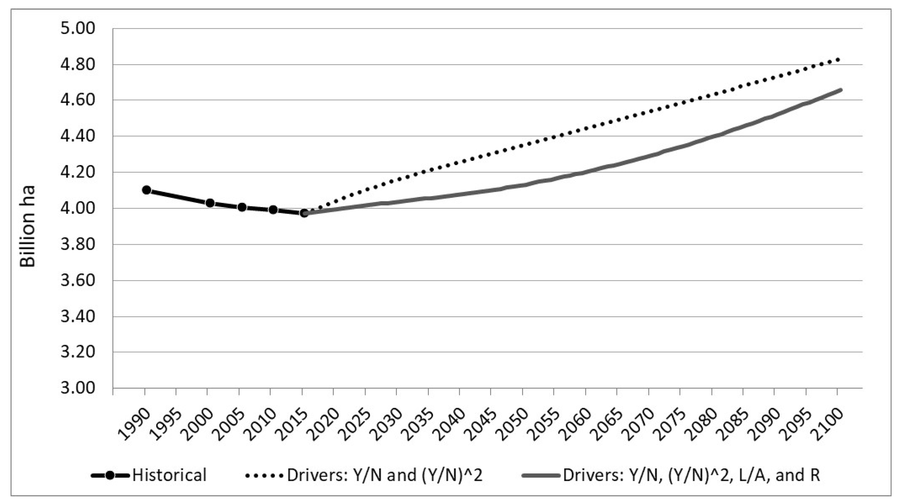
A few past studies that employed the EKC model in projecting global forest area used only Y/N and (Y/N)
2 as drivers, keeping all the other variables constant at the base year level, e.g., as routinely done in the Global Forest Products Model (GFPM) [
14,
26]. To enable better comparisons with those studies, we generated total forest area projections to 2070 for SSP2 driven only by Y/N and (Y/N)
2, keeping the effect of all the other variables constant at the current level (
Figure 3 and
Figure 4). These Y/N-only projections could be compared with projections made with the fuller specification. The comparison suggested how not including other important explanatory variables in the projections would produce biased results. For instance, the global projection of forest area in SSP2 was overestimated by 6% when R and L/A were not used to drive the projections. However, the differences in projections tended to decline and converge over time (
Figure 3). Such an upward bias in projection was also true for Africa (4a), North America (4d), and Oceania (4e), which showed up to 24%, 11%, and 16% higher forest area projections in the SSP2 scenario for these three regions, respectively. In contrast, the forest area projections for Asia (4b) and Europe (4c) were lower using the simpler model, by 6% and 3%, respectively, when projections were driven only by Y/N and (Y/N)
2. Finally, the differences for South America between the two projections were smaller, converging toward the end of the projection. Overall, the results obtained by including R and L/A appear more plausible, given that it more closely captured the most recent trends in forest area in all countries and regions, with less drastic projected changes in future as seen in
Figure 3 and
Figure 4a–f.
Next, we compared our projected forest area for SSP2, with projections produced by the 2017 version of GFPM through 2070, which was driven by only Y/N and (Y/N)
2. The 2017 version of GFPM [
27] used in projecting forest area in this study specifies the effect of Y/N and (Y/N)
2 on forest area annual growth rate as 0.0014 and −0.0898, respectively. The comparison (not shown) indicated that our projected global forest area was 9% higher in 2070, when only Y/N and (Y/N)
2 were used to drive the projection, but only 4% higher when R and L/A were additionally used to drive the projection. These projection differences between the two models were up to 1% for North America, 2% for Asia, 14% for South America, and 34% for Africa, with our model generating higher values than the GFPM projections.
Despite differences in the magnitudes of projected forest areas, our projected trends in global and regional forest area trends are consistent with the future expectation that forest area is on a path toward overall global increases, which is mainly due to advancement in technologies, rural migration to cities, and economic growth. This vision is also in line with perspectives offered by others (e.g., [
28]), which have argued that forests are set to recover because of improved forestry methods, the spread of advanced forest governance, and global cooperation and policy.
One key observation based on our projections of total forest area driven only by income per capita and its square values indicates an immediate increase in forest area for all the studied countries and regions, suggesting that the income turning point has already been reached. This increasing trend occurs with any income above $270, which is much lower than the values that past studies have indicated (e.g., more than $800). The seemingly early turning points indicated by our model are expected, since we used all the countries to estimate one single model, rather than estimating separate models for more homogenous country groups. Therefore, our model should be best used to understand the relationship between different explanatory variables and forest area rather than using it to estimate specific turning points.
While our estimated EKC model of forest area captures the effect of important economic and demographic factors and the forest area outlook obtained using the estimated model is consistent with the assumed future changes in economic and demographic variables, caveats should be noted with our model estimates. First, our results might have suffered from the exclusion of other variables in our model, such as policy and institutional factors (e.g., see [
7]). Our results do not explicitly consider competition for land between various uses, which is mainly determined by the economics of each land use (e.g., land rent). For instance, increasingly richer populations with changing diet preferences (e.g., more meat consumption) in the future may lead to increased demand for land for food and feed production, leading to either deforestation or no land area available for afforestation/reforestation (e.g., see [
29]). Similarly, increasing future demand for wood energy may lead to increased wood prices, which may drive up forestland rents (the profitability of forestland) and thereby limit forestland conversion to other uses, (e.g., see [
30]). Alternatively, higher bioenergy prices may lead to the conversion of natural forests or timber-oriented plantations to short rotation woody or herbaceous bioenergy crops (e.g., see [
31]).
We also acknowledge that forest area EKC modeling, without distinguishing between natural and planted forests, may have contributed to some uncertainties. Total forest area is the sum of natural forests and planted forests, and in reality, natural forests and planted forests are not necessarily driven by the same microeconomic, social, and policy factors [
6]. For instance, while the expansion (or contraction) of planted forests is driven mainly by economics [
32], natural forest area is more directly affected by demands for various ecosystem services and regional economic development goals. Future research could provide an improved understanding of the relationship between income and planted and natural forest areas.
The lack of distinction between natural and planted forests in our EKC models suggests that the projected future changes in total forest area reported in this study may not necessarily imply a proportionate increase in climate change mitigation benefit. The recent data indicate rising trends for planted forest area and declining trends for natural forest area [
20]. If such trends are to continue into the future, it is important to emphasize that compensating planted forest carbon gains will lag natural forest deforestation carbon losses while young planted trees grow, which is a process than can take several decades to play out. The long-term climate change mitigation benefits of increasing forest area also depend on the actual impacts of climate change on forest growth, which could be either positive, for example, due to increasing CO
2 fertilization, growing season lengthening, and precipitation increases, or negative, due to greater water stresses brought about by higher temperatures.


