Building a Social Discount Rate to be Applied in US Afforestation Project Appraisal

Abstract

This paper is focused on searching for the suitable discount rate to be applied to the valuation of a project related to forests in the USA, e.g., a recreational area inside a national park. To do this, we propose a new model based on hazard rate concepts, i.e., based on the risk that waiting time implies. More specifically, we derive the discount function whose instantaneous discount rate is the hazard rate of the system supporting the investment. We determine the rate of failure corresponding to different partition criteria of the whole system; in our case, we can use the information on forest fires caused in different ways, in different states or in different types of forest surfaces. After showing independence between the forest fires by states and causes, we derive a specific discount function for each cause which can be applied to every state or set of states which agree to fight against a concrete cause of forest fire. Additionally, we obtain a unique discount function by weighting the partial discount functions by type of forest surfaces. Our results are in line with the recommendations from several authors about using decreasing discount rates for projects with very long-term impacts.

1. Introduction

When we face the problem of valuing a public project, there are two important problems to deal with. First, which non-monetary benefits and costs to include and how to monetize them. And second, which discount rate—or even which discount function—to use in the project appraisal. In the case of public projects, this discount rate is called the social discount rate. Following [1], “[s]ocial discount rate (SDR) is used by society to give relative weight to social consumption or income accruing at different points in time.” We shall focus on this second problem because as [2] (p. 788) pointed out “few topics in our discipline rival the social rate of discount as a subject exhibiting simultaneously a very considerable degree of knowledge and a very substantial level of confusion”.

Traditionally, two benchmarks have been used to calculate the social discount rate, namely the social opportunity cost rate of capital and the social time preference rate.

The social opportunity cost of capital is usually identified with the real rate of return earned on a marginal project in the private sector. In [3], we find an interesting application of this opportunity cost of capital method to obtain an appropriate social discount rate to appraise public forestry investments.

The social time preference rate (STPR) is the rate of fall in the social value of consumption by the public. It is also known as the consumption rate of interest.

In practice, public projects are evaluated by means of a cost–benefit analysis (CBA). The concept of CBA is attributed to [4], and in [5] a historical overview of the CBA can be found. In CBA, compound interest is used to calculate the net present value (NPV) of the project or an exponential discount function that implies a constant discount rate, which is the same thing. For example, the European Commission [6] recommends the use of the exponential discounting model and a constant 5% European social discount rate for the Cohesion Fund eligible countries and 3% for the others (countries non-eligible for the Cohesion Fund). Since 1994, the US government had maintained a policy that its agencies use a real discount rate of 7% as a base-case for their CBA analyses (Office of Management and Budget [7]). In 2003, this rate was updated and the US Office of Management and Budget (OMB) recommended using a 3% rate along with the 7% rate for sensitivity analyses [8]. In case of having important intergenerational benefits or costs, a lower but positive discount rate is used in addition to calculating net benefits using discount rates of 3 and 7 percent. As a general rule, a constant SDR is proposed in practice to value public projects. Nevertheless, the UK and French governments, in line with the proposals of several authors for long-term valuations, have decided to use declining discount rates. The UK Green Book [9] proposes a SDR of 3.5% (based on the calculation of the social time preference rate). It also establishes a decreasing sequence of rates for projects with very long-term impacts (more than 30 years), and the circumstances where exceptions to the recommended rates are allowed. In France, the discount rate was lowered from 8% to 4% (in real terms). It has also been decided to use a decreasing discount rate for very long-term evaluations (horizons of more than 30 years) with a 2% discount rate as a minimum (Commisariat Général du Plan [10]).

In the appraisal of very long-term projects, like environmental projects, with impacts on future generations, several authors have proposed time declining discount rates. Against this single rate hegemony, dissident voices have been raised for many years. For example, according to [11], ‘‘new work suggests powerful reasons why the discount rate is not a single number, but a number that varies in a declining fashion with time. This result emerges from several approaches: from an analysis of how people actually discount the future (hyperbolic discounting and other functional forms); from the implications of uncertainty about the future (the Weitzman and Gollier approaches); and from an explicit attempt to replace the traditional present value maximand of policy appraisal with one that incorporates that goal along a sustainability requirement’’. For a revision of these approaches and the contributions of time declining discount rates, see [12,13,14]. In the same vein, there are recent interesting contributions from [15,16,17,18].

Focusing on the uncertainty about the future approach, there are several reasons for risk-adjustment of the social discount rate, depending on the consideration of uncertainty. Following [19], we must distinguish between uncertainty regarding the economic environment in general, which gives rise to the precautionary or insurance-like aspect of investments as a means of hedging against this macroeconomic risk [20], the uncertainty about the project’s future costs and benefits, and their relation to other income accruing to households which can be accounted by the covariance between project returns and the economic development in general. There are interesting proposals of risk-adjusted social discount rates [19,21] which build on the Weitzman approach [22,23] consisting of a linear decomposition of the project returns into one part that is correlated with the overall economic activity, and another part that is independent of it, having as a result discount rates declining over time at a rate which depends on the portion of covariant risk.

Our problem here is: How should we approach the problem of building a social discount rate? We propose a method based on the hazard rate of the investment that could be included in the uncertainty about the future approach and which leads to variable discount rates. We consider the investment project as a system and its possible hazards or fails, depending on the nature of the project. We find a similar survival approach in [24,25] that estimate the pure time preference rate starting from the calculus of life expectancy and its projection over the investment time horizon. But we shall consider the hazard rate of the investment itself, instead of considering the hazard rate (mortality) of the population for which the project is launched.

After this introduction, in the next section we define the basics of hazard rates and discounting. In Section 3 we develop the empirical application to obtain the appropriate discount rates, starting by explaining the data we use and how we obtained them. Finally, in Section 4 we analyze the results, summarize, and conclude.

2. The Hazard Rate Approach: Concepts and Equations

We focus first on the risk implicit in the discounting of delayed rewards. We can simply state that the value of a future reward is discounted because of the risk that waiting for its receipt implies. The discount function can be decomposed into several components. In the framework of a constant social discount rate, these components are usually given by the Ramsey [26] formula. In [27] we find a more detailed analysis of the parameters of the Ramsey formula.

We shall adopt the following simplifying assumption: any discount function can be decomposed into the product of the discount function derived from the hazard rate and the discount function due to the remainder of the causes (pure time preference rate, growth of per capita consumption, etc.). Therefore,

$$F(t)=\widehat{F}(t)\cdot \tilde{F}(t),$$

(1)

where:

• $\widehat{F}(t)$ represents the discount function derived from the hazard rate of the system, and
• $\tilde{F}(t)$ denotes the discount function due to the rest of the causes involved in the valuation process.

However, in this paper, we only consider the problem of determining the discounting function $\widehat{F}(t)$, leaving the study of the influence of the rest of the causes for future research.

In a revision of the literature on hazard rate and discounting, we find the works [12,28,29,30,31,32,33,34]. Green and Myerson [28] (p. 498), comparing the exponential and the hyperbolic functions, provided this interesting result: “The hazard rate for the exponential discounting model is constant: each additional unit of waiting time adds a constant amount of additional risk. In contrast, the hazard rate from the hyperbolic discounting model decreases with time. In fact, this hazard rate decreases hyperbolically, with each additional unit of waiting time adding successively smaller amounts of risk”. Sozou [29] also attributes a decreasing hazard rate to the use of hyperbolic discounting but in an exponential way since the prior distribution of the hyperbolic hazard rate is an exponential function.

A hazard function describes mathematically the effect that increases in waiting time have on the risk that something will happen to prevent an event from occurring [35]. In the framework of temporal discounting, the fail represents the probability of an event occurring at t (or during an interval starting at t) that will prevent the receipt of a reward, divided by the probability of the event not occurring until t, that is the conditioned probability of failure.

Let T be the random variable that represents the life of an investment in a public good, for example, a forest or a natural park. It is well known that the distribution function of the random variable, $F_T(t)=P(T\le t)$ (with density function $f_T(t)$), represents the probability that the public good will stop working before t years after starting its useful life (time 0). The reliability of the system at year t, $R(t)$, is the probability that the life of the system will be greater than t:

$$P(T>t)=1-F_T(t)=R(t), t > 0.$$

(2)

Therefore,

$$h(t)=\frac{f_T(t)}{R(t)}$$

(3)

represents the proportion of units that fail in the interval $(t,t+\mathrm{d}t)$ with respect to the units that continue working at year t. This is the well-known concept of hazard rate, and it can be shown that:

$$h(t)=-\frac{R^{\prime }(t)}{R(t)}.$$

(4)

We propose a discount function for investment appraisal based on the system reliability. So, the discount function at t will be [12]:

$$R(t)=1-F_T(t)=e^{-{\displaystyle \underset{0}{\overset{t}{\int }}h(x)\mathrm{d}x}}.$$

(5)

Then, we can make the hazard rate of a random variable equal to the instantaneous rate of the discount function [12]:

$$F(t)=1-F_T(t)=R(t), t\ge 0.$$

(6)

Our findings can also be derived from Gollier [36,37]. See [12] for a complete demonstration.

We have just described the univariate hazard rate of a system, but we could also consider a multivariate hazard rate. For example, taking the case of an investment in reforestation, we could consider the forest fire as the fail of the system. But this fail (the fire) can be due to several causes (arson, lightning, etc.). So our problem now is how to aggregate several hazard rates in a single hazard rate. We shall use a simple method, considering the approach of Barlow and Proschan [38] for structures of non-identical components. More specifically, we focus on the particular case when the system hazard rate is the sum of the weighted hazard rates, h_k of the n system components, that is:

$$h={\alpha }_1\cdot h_1+{\alpha }_2\cdot h_2+\cdots +{\alpha }_n\cdot h_n={\displaystyle \sum _{k=1}^n{\alpha }_k\cdot h_k},$$

(7)

where ${\alpha }_k$ are the weighting factors.

Taking into account that the general structure of the system failure has the following form [33]:

$$h(t)={\displaystyle \sum _{k=1}^n\frac{R_k\cdot \partial R/\partial R_k}{R}}\cdot h_k(t),$$

(8)

one has:

$$R=R_1^{{\alpha }_1}\cdot R_2^{{\alpha }_2}\cdots R_n^{{\alpha }_n}={\displaystyle \prod _{k=1}^n{R}_k^{{\alpha }_k}}.$$

(9)

This is the formula we will use to calculate the multivariate discount function based on the relationship between hazard rate and instantaneous discount rate, previously shown in Equation (6).

In general, the methodology proposed in this paper is appropriate when calculating the discount rate in real problems or situations involving failures. In this way, the hazard rate becomes a suitable tool to value the idiosyncratic or unsystematic part of the discount rate, that is to say, the component of the discount rate due to the risk of the specific investment project under appraisal. This is the case of the investment in forests where the existence of forestry problems (such as fires and pests) is a noteworthy component of the discount rate to be applied, similarly to the rate of mortality in populations.

Nevertheless, in this paper we focus on the appraisal of public forestry investments, and we apply the methodology to calculate the part of the discount function due to the hazard rate derived from forest fires; but this methodology could be applied as well to other forestry problems, such as pests.

According [39], “The vast literature on finance […] is in favor of using different discount rates to value different investment projects as a function of their degree of riskiness”. Our methodology can be applied to any forest issue, but it is necessary to adapt it to the specific hazard considered.

3. An Empirical Application

3.1. The Data

3.1.1. US Land Management and Forest Fire Data

The total land area of the USA is approximately 2.3 billion acres. The first public domain dates from 1781 and, over the next century, the Federal Government steadily increased its landholdings. Amongst the more famous public lands that have remained exempt from disposal for development have been Yellowstone National Park and Grand Canyon National Park (Bureau of Land Management [34]). A range of agencies has been created to hold and manage US public lands.

The following federal agencies are partners of the US National Interagency Fire Center (NIFC) (https://www.nifc.gov/):

• Bureau of Land Management (BLM)
• U.S. Fish and Wildlife Service
• National Park Service
• U.S. Forest Service (USFS)
• National Oceanic and Atmospheric Administration
• National Business Center
• U.S. Fire Administration
• National Association of State Foresters
• Bureau of Indian Affairs
• Department of Defense
• Fish and Wildlife Service
• National Park Service

Of these, the two largest agencies are the Bureau of Land Management (BLM) (http://www.blm.gov/wo/st/en.html) and the U.S. Forest Service (USFS) (http://www.fs.fed.us/), which were also the only two agencies with detailed fire cause data. On the advice of the NIFC we have proceeded with the data from the BLM and USFS only. The NIFC logic was based on the fact that in 2012 the federal government owned roughly 635–640 million acres, 28% of the 2.27 billion acres of land in the United States. In the same year the BLM, which has a multiple-use, sustained-yield mandate that supports a variety of uses and programs, including energy development, recreation, grazing, wild horses and burros, and conservation, managed about 247.3 million surface acres of public land across 42 states [40]. And the USFS, most of whose lands under management are designated National Forests, managed 193 million acres across 40 states, also for multiple uses and sustained yields of various products and services, including timber harvesting, recreation, grazing, watershed protection, and fish and wildlife habitats. Together, therefore, in 2012 these two agencies managed 67% of total Federal land [41].

3.1.2. The Bureau of Land Management (BLM)

As we have already explained, we are going to use data on forest fires from the BLM and the USFS. In Table 1 we can see the forest surface managed by the BLM by country for the years 2002 and 2012.

Table 1. BLM acreage data and percentage by state in 2002 and 2012. Source: Bureau of Land Management (BLM) of the US.

	Acres 2002	Acres 2012	% 2012 Total	2012 as % of 2002 Acreage
Alaska	86,500,000	72,423,478	29.33%	83.73%
Arizona	14,300,000	12,204,355	4.94%	85.35%
California	14,600,000	15,338,434	6.21%	105.06%
Colorado	8,400,000	8,335,283	3.38%	99.23%
Idaho	11,900,000	11,612,234	4.70%	97.58%
Montana	8,000,000	7,985,237	3.23%	99.82%
Nevada	47,900,000	47,783,458	19.35%	99.76%
New Mexico	13,400,000	13,466,922	5.45%	100.50%
Oregon	16,200,000	16,138,333	6.54%	99.62%
Utah	22,800,000	22,854,555	9.26%	100.24%
Washington	400,000	429,088	0.17%	107.27%
Wyoming	18,400,000	18,375,736	7.44%	99.87%
Total	262,800,000	246,947,113	100%	93.97%

There are BLM land holdings in other, eastern states but they are relatively small and have been ignored for the purpose of calculating hazard rates. In fact, some states are amalgamated, for example Nebraska is included in the Wyoming data, Texas in New Mexico, and both North and South Dakota with Montana. This is because the BLM does not always have exact latitude and longitude data for fires that may overlap state boundaries.

Figure 1 shows the burnt forest surface by state managed by the BLM, from 2002 to 2012. BLM fire data are available annually for human caused and natural (mainly lightning) caused fires. In addition, there are fires with unknown causes. This enables a multivariate analysis to be carried out using three variables: human, natural, and unknown.

Figure 1. BLM fire data by state in the period 2002–2012. Source: Bureau of Land Management (BLM) of the US.

3.1.3. United States Forest Service (USFS) Data

USFS area data are available for total and National Forests, which would enable a separate hazard rate to be calculated for National Forests, or even an individual forest if it for example exhibited different fire rates than others.

From Table 2 it is evident that with the exception of Nebraska, all states exhibited less than 10% variation in USFS total acreage between 2002 and 2012. Nevertheless for our analysis each separate year total has been used as the denominator in the loss percentage.

Table 2. USFS acreage data and percentage by state in 2002 and 2012. Source: United States Forest Service (USFS).

	Acres 2002	Acres 2012	% 2012 Total	2012 as % of 2002 Acreage
Alabama	1,288,079	1,288,251	0.55%	100.01%
Alaska	24,355,135	24,359,118	10.46%	100.02%
Arizona	11,890,608	11,891,457	5.11%	100.01%
Arkansas	3,539,672	3,552,891	1.53%	100.37%
California	24,429,950	24,443,800	10.50%	100.06%
Colorado	16,014,877	16,034,994	6.89%	100.13%
Florida	1,433,601	1,434,931	0.62%	100.09%
Georgia	1,857,649	1,857,785	0.80%	100.01%
Idaho	21,652,055	21,658,427	9.30%	100.03%
Illinois	856,686	923,271	0.40%	107.77%
Indiana	644,362	644,269	0.28%	99.99%
Kansas	116,319	116,319	0.05%	100.00%
Kentucky	2,211,710	2,208,164	0.95%	99.84%
Louisiana	1,024,637	1,024,637	0.44%	100.00%
Maine	93,293	93,293	0.04%	100.00%
Michigan	4,894,424	4,894,251	2.10%	100.00%
Minnesota	5,466,802	5,466,806	2.35%	100.00%
Mississippi	2,320,273	2,317,877	0.99%	99.90%
Missouri	3,060,166	3,060,162	1.31%	100.00%
Montana	19,109,744	19,144,890	8.22%	100.18%
Nebraska	442,492	560,492	0.24%	126.67%
Nevada	6,275,437	6,275,796	2.70%	100.01%
New Hampshire	828,111	828,356	0.36%	100.03%
New Mexico	10,455,455	10,457,197	4.50%	100.02%
New York	16,211	16,259	0.01%	100.30%
North Carolina	3,167,566	3,165,378	1.36%	99.93%
North Dakota	1,105,981	1,106,694	0.48%	100.06%
Ohio	834,173	834,173	0.36%	100.00%
Oklahoma	772,383	754,689	0.32%	97.71%
Oregon	17,501,788	17,579,887	7.55%	100.45%
Pennsylvania	742,935	742,936	0.32%	100.00%
South Carolina	1,378,844	1,378,520	0.60%	99.98%
South Dakota	2,368,694	2,452,381	1.05%	103.53%
Tennessee	1,276,319	1,276,084	0.55%	99.98%
Texas	1,994,732	1,994,473	0.86%	99.99%
Utah	9,208,643	9,213,074	3.96%	100.05%
Vermont	817,298	822,700	0.35%	100.66%
Virginia	3,224,034	3,223,324	1.38%	99.98%
Washington	10,110,507	10,115,211	4.34%	100.05%
West Virginia	1,869,374	1,896,403	0.81%	101.45%
Wisconsin	2,022,980	2,022,984	0.87%	100.00%
Wyoming	9,703,495	9,706,283	4.17%	100.03%
Total	232,377,494	232,838,887	100.00%	100.20%

Figure 2 shows the burnt forest surface by state managed by the USFS, from 2002 to 2012.

Figure 2. USFS fire data by state in the period 2002–2012.

USFS fire data are available annually. There are major variations in the area burned by state in individual years. The USFS fire data were made available by cause and area in more detail—nine different causes are provided (see Table 3). Of these, eight are human in origin: arson, campfire, children, debris burning, use of equipment, railroad, smoking, and miscellaneous (e.g., power lines). Only lightning is a natural cause. These data are available for all states where USFS keeps records.

Table 3. Sample of USFS fire cause data: California, 2012. Source: United States Forest Service (USFS).

	National Forest (Acres)	Total All Land (Acres)
Arson	1794	2168
Campfire	76,716	76,767
Children	6	6
Debris Burning	16	61
Equipment Use	5550	5612
Lightning	76,401	76,760
Miscellaneous	38,272	39,169
Railroad	3	4
Smoking	2	3
Human Total	122,359	123,790
Non Human Total	76,401	76,760
Total	198,760	200,550

However, we have grouped these causes, in order to deliver consistency with the BLM data, where we had human, natural, and unknown causes. Lightning has been characterized as natural, whereas the other causes are ‘human’, except miscellaneous. The cause miscellaneous has been labeled as the ‘unknown’ category, since it is impossible to know the nature, human or natural, of each fire included in this category.

3.1.4. Data Selection and Analysis

Both sets of fire data were provided to us for the decade 2002 to 2012; full BLM but only partial USFS 2013 data were provided, therefore the data series used was 2002–2012. The data extracted were for the area burned (the loss), not the number of fires. Nevertheless it is worth observing that the distribution curve of fires by size is far from even; a few fires make up a very large proportion of the overall total. This may have significant local policy implications that are not revealed in the hazard rate calculation.

3.2. Analysis of the Variables Involved in Forest Fires

As we have stated previously, we are looking for a multivariate discount function based on the relationship between hazard rate and instantaneous discount rate. We use data on forest fires by cause and state from 2002 to 2012 in order to calculate discount functions for every state (with global data for all the causes) or for every cause (with global data for all the states). For this reason, we first use the chi square to test the relationship between the variables “cause of burning” and “state” for significance. 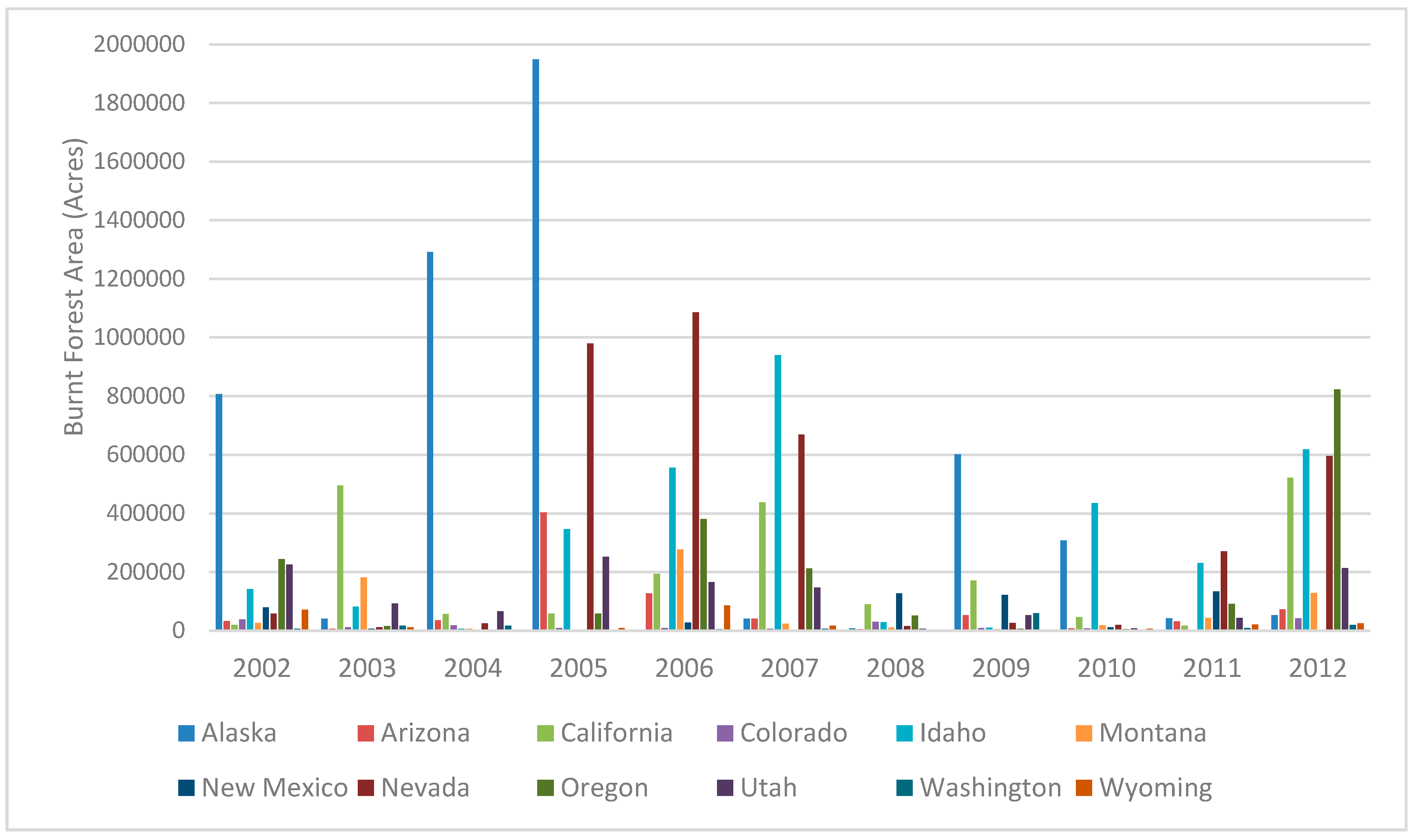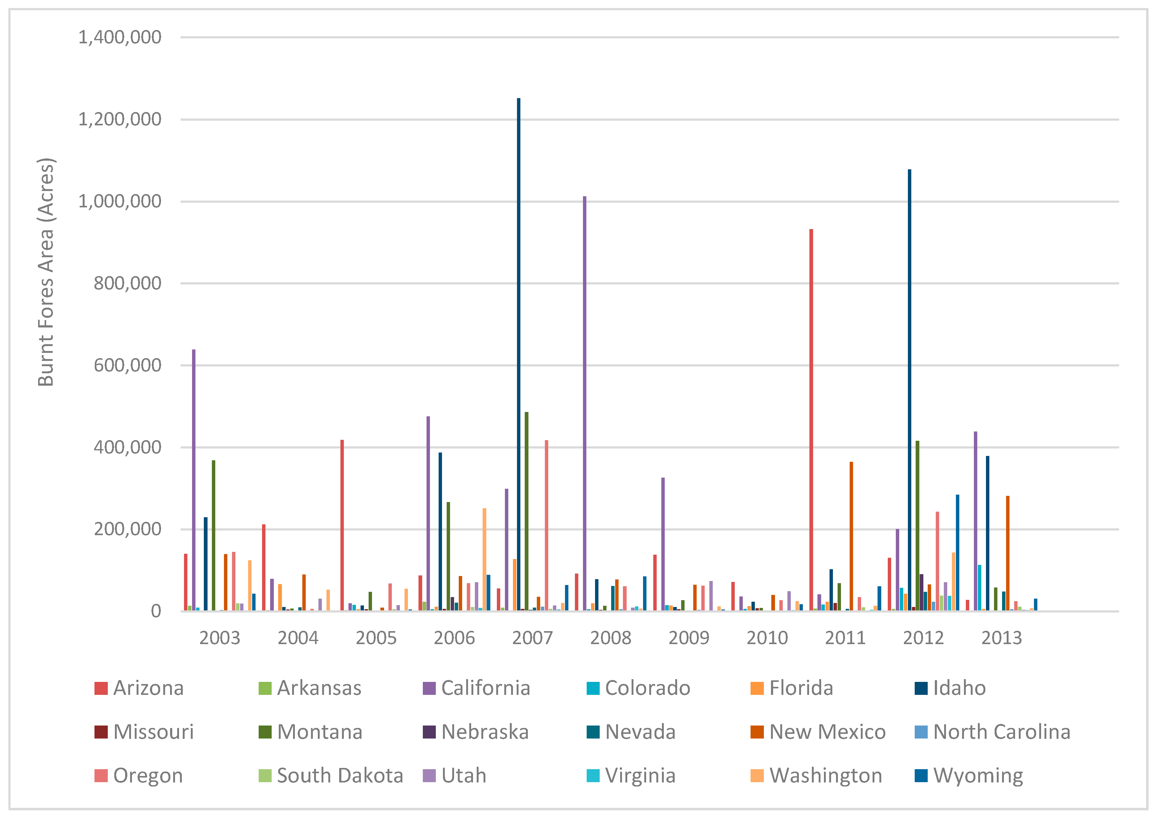In effect, Table 4 shows the data for the number of burned acres by state and cause.

Table 4. Observed frequencies for fire causes and states (number of burned acres). Source: Own elaboration with data from BLM and USFS.

	Causes (Observed)			Total
States	Human	Natural	Unknown	(ni.)
Alabama	15,649.98	1,954,872.76	3946.66	1,974,469.40
Alaska	252,412.70	3,346,983.70	45.60	3,599,442.00
Arizona	843,521.96	1,293,639.25	558,774.75	2,695,935.96
Arkansas	485,609.18	147,785.06	55,873.56	689,267.80
California	2,502,075.43	2,033,309.58	863,666.13	5,399,051.14
Colorado	134,476.60	476,270.34	294,075.95	904,822.89
Florida	95,275.95	190,205.64	57,253.43	342,735.02
Georgia	6536.28	39,589.95	7926.47	54,052.70
Idaho	567,058.04	5,176,511.03	153,284.91	5,896,853.98
Illinois	149,392.24	869,139.05	61,968.08	1,080,499.37
Indiana	805.86	19.70	231.41	1056.97
Kansas	21,625.67	53.25	49.81	21,728.73
Kentucky	27,470.29	2611.81	3364.23	33,446.33
Louisiana	15,874.22	5083.31	8956.67	29,914.20
Maine	40.10	0.00	0.00	40.10
Michigan	20,780.66	319.91	3318.16	24,418.73
Minnesota	77,654.29	134,669.73	1833.43	214,157.45
Mississippi	13,952.05	2931.12	35,660.85	52,544.02
Missouri	53,834.95	244.48	9358.11	63,437.54
Montana	111,358.66	1,939,108.62	110,538.63	2,161,005.91
Nebraska	7096.05	433,482.24	14,770.55	455,348.84
Nevada	212,719.69	3,773,952.52	23,544.36	4,010,216.57
New Hampshire	61.80	46,628.51	570.28	47,260.59
New Mexico	354,107.41	1,092,463.35	315,899.56	1,762,470.32
New York	857.25	64,152.58	53.05	65,062.88
North Carolina	16,542.75	11,295.75	26,897.25	54,735.75
North Dakota	9026.50	8641.59	1208.33	18,876.42
Ohio	2294.06	2.00	858.32	3154.38
Oklahoma	27,570.73	4456.85	4954.50	36,982.08
Oregon	256,884.27	3,440,626.11	100,636.75	3,798,147.13
Pennsylvania	292.74	9.90	325.75	628.39
South Carolina	12,014.06	1777.83	5688.46	19,480.35
South Dakota	23,708.48	63,960.45	26,375.03	114,043.96
Tennessee	15,322.29	8644.41	3249.30	27,216.00
Texas	7511.61	11,235.80	1869.45	20,616.86
Utah	199,520.87	1,433,748.97	107,795.57	1,741,065.41
Vermont	51.29	0.10	2.50	53.89
Virginia	41,714.30	11,469.42	23,397.96	76,581.68
Washington	116,244.33	693,560.52	95,557.11	905,361.96
West Virginia	1479.63	178.87	1726.81	3385.31
Wisconsin	275.05	155.60	1545.38	1976.03
Wyoming	99,854.46	762,889.38	104,039.06	966,782.90
Total (n.j)	6,800,554.73	29,476,681.04	3,091,092.17	39,368,327.94

The question is whether there is a significant relationship between cause and state. To determine this, we shall follow these steps:

First, state the null hypothesis: there is no relationship between fire cause and state. We test this hypothesis using contingency tables.

Second, compute the expected frequency for each cell based on the assumption that there is no relationship. These expected frequencies are computed from the totals shown in Table 4 as follows:

$$e_{ij}=\frac{n_{i\cdot }{n}_{\cdot j}}{n},$$

(10)

where $e_{ij}$ is the expected frequency for cell $(i,j)$, $n_{i\cdot }$ is the total for the i-th row, $n_{\cdot j}$ is the total for the j-th column, and n is the total number of observations, in our case 39,368,327.94. As an example, we could calculate the expected frequency for the number of burnt acres due to human causes in Alabama:

$$\begin{array}{c}{e}_{11}=\frac{\mathrm{Total} \mathrm{acres} \mathrm{burnt} \mathrm{in} \mathrm{Alabama} \times \mathrm{Total} \mathrm{acres} \mathrm{burnt} \mathrm{due} \mathrm{to} \mathrm{human} \mathrm{causes}}{\mathrm{Total} \mathrm{acres} \mathrm{burnt} (\mathrm{due} \mathrm{to} \mathrm{all} \mathrm{the} \mathrm{causes} \mathrm{in} \mathrm{all} \mathrm{the} \mathrm{states})}=\\ \frac{1,974,469.40\cdot 6,800,554.73}{39,368,327.94}=341,073.34.\end{array}$$

Table 5 shows the expected frequencies for each cause in all the states.

Table 5. Expected frequencies for fire causes and states (number of burned acres). Source: Own elaboration with data from BLM and USFS.

	Causes (Expected)
States	Human	Natural	Unknown
Alabama	341,073.34	1,478,366.18	155,029.87
Alaska	621,773.99	2,695,049.79	282,618.23
Arizona	465,700.75	2,018,557.77	211,677.43
Arkansas	119,065.34	516,083.06	54,119.40
California	932,641.66	4,042,490.92	423,918.56
Colorado	156,300.71	677,477.99	71,044.19
Florida	59,204.65	256,619.76	26,910.61
Georgia	9337.16	40,471.47	4244.07
Idaho	1,018,633.01	4,415,216.32	463,004.66
Illinois	186,647.38	809,014.17	84,837.82
Indiana	182.58	791.40	82.99
Kansas	3753.46	16,269.19	1706.08
Kentucky	5777.58	25,042.64	2626.11
Louisiana	5167.43	22,397.99	2348.78
Maine	6.93	30.02	3.15
Michigan	4218.13	18,283.30	1917.29
Minnesota	36,993.94	160,348.46	16,815.05
Mississippi	9076.55	39,341.86	4125.61
Missouri	10,958.31	47,498.29	4980.94
Montana	373,295.99	1,618,033.72	169,676.20
Nebraska	78,657.77	340,938.34	35,752.73
Nevada	692,731.92	3,002,613.55	314,871.11
New Hampshire	8163.88	35,385.94	3710.77
New Mexico	304,452.25	1,319,633.78	138,384.29
New York	11,239.08	48,715.25	5108.56
North Carolina	9455.15	40,982.90	4297.70
North Dakota	3260.75	14,133.55	1482.12
Ohio	544.89	2361.81	247.67
Oklahoma	6388.35	27,690.00	2903.73
Oregon	656,098.67	2,843,828.46	298,220.00
Pennsylvania	108.55	470.50	49.34
South Carolina	3365.07	14,585.74	1529.54
South Dakota	19,700.16	85,389.39	8954.42
Tennessee	4701.34	20,377.73	2136.93
Texas	3561.39	15,436.69	1618.78
Utah	300,754.72	1,303,607.05	136,703.64
Vermont	9.31	40.35	4.23
Virginia	13,228.86	57,339.84	6012.98
Washington	156,393.83	677,881.61	71,086.52
West Virginia	584.78	2534.72	265.81
Wisconsin	341.34	1479.53	155.15
Wyoming	167,003.79	723,869.99	75,909.12

Third, compute the chi square and degrees of freedom. The significance test is conducted by computing the chi square as follows:

$${\chi }_{\exp }^2={\displaystyle \sum _{i=1}^{42}{\displaystyle \sum _{j=1}^3\frac{{(e_{ij}-n_{ij})}^2}{e_{ij}}}}=12,842,165.33.$$

(11)

On the other hand, the number of degrees of freedom is equal to $(r-1)(c-1)$, where r is the number of rows and c is the number of columns. In this case, the number of degrees of freedom is $(42-1)(3-1)=82$. As the theoretical value of the chi square, ${\chi }_{82}^2$, at a 95% significance level is located between 101.879 and 107.522, we can deduce that the null hypothesis of no relationship between fires cause and state can be rejected.

Given this result, we have to study next the degree of association between these two variables. We follow [42] to explain several coefficients to assess the degree of association between two variables, “none of which appears to be completely satisfactory”:

1. Pearson’s contingency coefficient, P, defined by:

$$P=\sqrt{\frac{{\chi }_{\exp }^2}{{\chi }_{\exp }^2+n}}.$$

(12)

Its value is located between 0 and $P_{\max }=\sqrt{\frac{h-1}{h}}$, where $h=\min \{r,c\}$. In our case, $P_{\max }=\sqrt{\frac{2}{3}}=0.82$ and $P=0.50$. So, there exists a certain association between both variables. This coefficient has the disadvantage that, even in the case of complete association, the value of P depends on the number of rows and columns. To solve this restriction the following coefficient has been suggested.

2. Tschuprow’s contingency coefficient, $T^2$, defined by:

$$T^2=\frac{{\chi }_{\exp }^2}{n\sqrt{(r-1)(c-1)}}.$$

(13)

It is located between 0 and 1, being 0 in case of complete independence. This only attains a value of 1 in the case of complete association when $r=c$ but cannot do so if $r\ne c$. In our example, $T^2=0.04$.

In the following modification suggested by Cramer, the unity can be obtained for all values of r and c in the case of complete association.

3. Cramer’s contingency coefficient, C, defined by:

$$C=\frac{{\chi }_{\exp }^2}{n(h-1)}.$$

(14)

Its value is located between 0 and 1. In our case, $C=0.16$.

These three suggested coefficients have no obvious probabilistic interpretation. The coefficient we introduce next is interpretable in a predictive sense. The rationale behind Goodman and Kruskal’s lambda measures is: “How much does a knowledge of the classification of one of the variables improve one’s ability to predict the classification on the other variable?” [43].

4. Goodman and Kruskal’s index of predictive ability lambda, ${\lambda }_B$, defined by:

$${\lambda }_B=\frac{{\displaystyle \sum _{i=1}^r\underset{j}{\max }}(n_{ij})-\underset{j}{\max }(n{.}_j)}{n-\underset{j}{\max }(n{.}_j)},$$

(15)

where $\underset{j}{\max }(n{.}_j)$ is the overall modal frequency of the dependent variable Y, and ${\displaystyle \sum _{i=1}^r\underset{j}{\max }}(n_{ij})$ is the sum of modal frequencies on the dependent variable Y within separate categories of the independent variable X. ${\lambda }_B$ is the relative decrease in the probability of an error in guessing the category of one variable, having information about the predictor variable. Its value is located between 0 and 1, being 1 when no error is made (and consequently there is complete predictive association). A disadvantage of the lambda measures is that the values of indices may be misleadingly low when the marginal distribution is far from being uniform [36].

In our example, one has ${\lambda }_B=\frac{30,539,956.13-29,476,681.04}{39,368,327.94-29,476,681.04}=0.11$. So we only have a decrease of 11% in the error made when guessing the cause of a fire produced in a certain state. This means that the association between the variables “state” and “cause of the forest fire” is low.

We think that, in our case, the independent variable should be the state and the dependent variable the cause. Nevertheless, and just to verify it, we can reverse the variables A and B. In this case, we will have ${\lambda }_A$, suitable for predictions of A form B:

$${\lambda }_A=\frac{{\displaystyle \sum _{j=1}^c\underset{i}{\max }}(n_{ij})-\underset{i}{\max }(n_i.)}{n-\underset{i}{\max }(n_i.)}.$$

(16)

In our case, we obtain ${\lambda }_A=0.08$. Despite the previously established limitations, both values are low. And we can complement these results with those obtained for the other indices we have previously calculated in order to state that there is a low association between the variables; therefore we can conclude and suppose in what follows that the variables are independent.

3.3. Calculation of Discount Rates

In the analysis presented in Section 3.2, we have statistically shown that there is no association between the causes of forest fires (1: human, 2: natural, and 3: unknown) and the states in USA (from Alabama to Wyoming) since the Goodman and Kruskal’s indexes are 0.11 and 0.08. Consequently, we can derive a discount function for each cause which can be applied to discount the social benefits generated by investment on reforestation either in a state, in a group of states, or all in states in the USA. More specifically, because of their suitability for modeling rates of increasing or decreasing hazard rates, we are going to use discount functions that belong to the family of generalized exponential discounting, defined by:

Before starting the process of fitting data, we have observed that the hazard rate corresponding to causes 1 and 3 is decreasing and so the hyperbolic discounting is appropriate to fit them. However, the hazard rate corresponding to cause 2 is increasing and so the hyperbolic discounting does not apply. For this reason, we have used instead the family of generalized exponential discount functions which, depending on the sign of one of its two parameters, can describe an increasing or decreasing discount rate.

$$F(t)=\exp (-\alpha t^{\beta }),$$

(17)

To calculate the values of α and β of this function, we use a linear regression, starting from the data of burnt forest surface due to cause i over the total forest surface. This way, we obtain the following results by causes (1, 2, and 3):

$$F_1(t)=\exp (-6.3326 t^{0.8502}),$$

(18)

$$F_2(t)=\exp (-5.4761 t^{1.1228}),$$

(19)

and

$$F_3(t)=\exp (-6.7074 t^{0.4993}).$$

(20)

Table 6 shows the estimated parameters of Equation (17) by using a linear regression and by reporting the results of the regression, specifically, the significance of coefficients.

Table 6. Significance of coefficients derived from Equation (17).

Cause 1
	Estimate	Std. Error	t-value	p-value
Intercept	−6.332592066	0.076418781	−82.866995955	2.7486 × 10−14 ***
Time	0.850169806	0.043855319	19.38578563	1.1953 × 10−8 ***
R-squared	0.976611754
Adjusted R-squared	0.974013061
Cause 2
	Estimate	Std. Error	t-value	p-value
Intercept	−5.476075401	0.105936811	−51.69190318	1.90587 × 10−12 ***
Time	1.122839569	0.060795168	18.46922401	1.83044 × 10−8 ***
R-squared	0.974293958
Adjusted R-squared	0.971437731
Cause 3
	Estimate	Std. Error	t-value	p-value
Intercept	−6.707351102	0.117163586	−57.24774522	7.62383 × 10−13 ***
Time	0.499265784	0.067238005	7.425350973	3.99477 × 10−5 ***
R-squared	0.859672838
Adjusted R-squared	0.844080931

Significance code: *** means “significant at 99.99% level”.

As indicated, they can be applied to every state or group of states which agree to fight against a concrete cause of forest fires for a given period (say from 2015 to 2030). Indeed, the discount rates using exponential discounting, deduced for each cause and year, are shown in Table 7.

Table 7. Discount rates per cause for the period 2015 to 2030.

Discount Rate (%)
Year	Human	Natural	Unknown
2015	0.119772	0.580446	0.032600
2016	0.118540	0.585399	0.031493
2017	0.117399	0.590071	0.030491
2018	0.116337	0.594493	0.029580
2019	0.115345	0.598693	0.028745
2020	0.114414	0.602693	0.027977
2021	0.113537	0.606513	0.027268
2022	0.112710	0.610169	0.026609
2023	0.111927	0.613675	0.025997
2024	0.111184	0.617045	0.025424
2025	0.110477	0.620288	0.024888
2026	0.109803	0.623415	0.024385
2027	0.109159	0.626434	0.023910
2028	0.108544	0.629353	0.023463
2029	0.107954	0.632179	0.023039
2030	0.107387	0.634918	0.022638

Observe that the discount rates for cause 2 (natural) are increasing, whilst the discount rates for causes 1 and 3 (human and unknown) are decreasing and that these percentages are only a part of the total discount rate to be applied per cause and year. As stated in Section 1, we have considered only the problem of determining the discount function derived from the hazard rate of the system, one of the two components of Equation (1) which displays the expression of the total discount rate.

In this paper, we have calculated the part of the discount rate due to the failure of forests caused by fires. Forest fire is just one of several forest investment hazards. Severe damages can be caused by pests, insects, grazing, air-borne pollution (such as ozone), soil acidification, etc. Following [44] the main hazards in forests are storms, snow, insects, and fire. But fire is a major disturbance to forests all over the world. On the other hand, in this paper the purely financial component of the discount rate has not been included since this is not the objective of this manuscript. The reason for using a diminishing component of the discount rate (due to fires) is because a decreasing hazard rate is expected, as is usual when studying the reliability of systems. In effect, [45] shows that the average area burned per year by forest fires in the five largest countries in southern Europe (France, Italy, Spain, Greece, and Portugal) has decreased during the period of 2000–2017. At this point, we must insist in that this paper only analyzes the component of the discount rate due to the hazard rate caused by fires and not the other components (financial, hazard rate due to pests, etc.) which, as just reported, must be diminishing. However, it is possible that the overall discount could be eventually increasing.

The equation to calculate the total discount rate for each cause i_k, taking into account Equation (1) and using exponential discounting, would be:

$$i_k(t)=F_k{(t)}^{-\frac{1}{t-2001}}\cdot (1+\tilde{i})-1,$$

(21)

where $F_k(t)$ is the discount function due to the k-th cause (k = 1, 2, and 3) and $\tilde{i}$ the discount rate due to the remainder of causes involved in the valuation process. Analogously, this analysis could be addressed by states and years instead of causes and years. In this case, the discount functions would be independent of causes and then a global policy without distinguishing among causes could be applied in each state.

Starting from the discount functions by causes, we could obtain a unique multivariate discount function using as weighting coefficients in Equation (10) the inverse of budgets intended to prevent each of the causes. Unfortunately, we do not have this information at our disposal, but we propose this idea and its possible application by decision-makers, when using a hazard approach in the valuation of forest investment.

Nevertheless, to illustrate how to calculate a multivariate discount function using our hazard rate approach, we will use the information on forest fires not by cause, but following the type of burned area (National Forests and the rest of forests), and the obtained discount functions will be weighted inversely proportional to the number of visitors to each area. We will use data from the USDA Forest Service [46] on registered visits to National Forests and to the rest of forests. From the available data on visits for the period 2008–2012, we have an annual estimation of 160,973,000 National Forest visits and 8,070,000 wilderness visits. This makes a total of 169,043,000 visits per year.

This way, our multivariate hazard rate will take into account the hazard rate for National Forests and the hazard rate for the rest of forests. So we have to take into account now the data on forest fires and forest surface from National Forests and from the rest of forests (see Table 8).

Table 8. Burnt surface and total forest surface of National Forests and the rest of forests. Source: USFS.

	National Forests			Rest of Forests
Year	Ha Total Burnt	Total Surface	% Burnt	Ha Total Burnt	Total Surface	% Burnt
2002	1,927,832	192,436,448	1.00%	115,058	39,941,046	0.06%
2003	1,540,486	192,482,838	0.80%	366,265	39,883,716	0.19%
2004	560,373	192,829,734	0.29%	29,382	39,603,330	0.02%
2005	632,246	192,614,172	0.33%	87,742	39,755,087	0.05%
2006	1,916,031	192,769,306	1.00%	69,613	39,568,634	0.04%
2007	2,888,193	192,710,830	1.50%	118,231	39,802,754	0.06%
2008	1,543,676	192,701,460	0.80%	29,444	39,850,376	0.02%
2009	749,503	192,769,177	0.39%	24,463	38,653,107	0.01%
2010	351,600	192,879,760	0.18%	15,832	39,737,256	0.01%
2011	1,633,631	192,892,534	0.85%	207,454	39,926,837	0.11%
2012	2,901,079	192,946,578	1.51%	102,700	39,892,309	0.05%

Following the same procedure as before, we obtain the hazard rate and then the global discount function (from the National Forest and the rest of forests discount functions). Using formulae (7) and (10), we have:

$$F(t)={[F_1(t)]}^{{\alpha }_1}{[F_2(t)]}^{{\alpha }_2},$$

(22)

where ${\alpha }_1=\frac{160,973,000}{169,043,000}$ and ${\alpha }_2=\frac{8,070,000}{169,043,000}$.

The discount rates, using exponential discounting, are shown in Table 9.

Table 9. Discount rates (due only to the hazard rate) from the global discount function (for National Forests and the rest of forests) for the period of 2015 to 2030.

Year	Discount Rate (%)
2015	0.700780
2016	0.696831
2017	0.693158
2018	0.689726
2019	0.686506
2020	0.683475
2021	0.680613
2022	0.677901
2023	0.675327
2024	0.672876
2025	0.670539
2026	0.668304
2027	0.666165
2028	0.664113
2029	0.662142
2030	0.660246

Observe that the obtained discount rates are decreasing over time and that these percentages are only a part of the total discount rate, as explained previously in the case of the discount rates per cause.

We could calculate the total discount rate i as we have done for the discount rates per cause. Thus, adapting Equation (21) we will have:

$$i(t)=F{(t)}^{-\frac{1}{t-2001}}\cdot (1+\tilde{i})-1,$$

(23)

where $F(t)$ is the global discount function and $\tilde{i}$ the discount rate due to the remainder of causes involved in the valuation process. As we have already noted, we are not going to analyze the discount function due to the remainder of causes. But, we think that, taking into account the literature reviewed in the introduction and the discount rates used by several governments, the discount rates due to the remainder of causes must be also decreasing, or at least constant, which will result in a decreasing total discount rate.

These results are in line with the recommendations from several authors about using decreasing discount rates for projects with very long-term impacts, as in the case of investments in afforestation. Specifically, in forestry financial analysis, we agree with Hepburn and Koundouri [14] in that “moreover forest managers will no doubt realize that the implementation of a declining discount rate scheme is not only important for the economic value of future timber products. It is also crucial in determining the net present value of forestry benefits that people derive from forest services, such as extraction of genetic material, tourism, protection of watersheds, support of other ecosystems, carbon storage, etc.”

Lastly, we would like to make a remark regarding the age of the forests. In our opinion, older forest stands have a greater probability of fire (less distance between trees, more near the cities, the majority of them are recreational areas, etc.). In effect, [47] recognize that the age distribution of stands in a region can be used to estimate the fire frequency by assuming a frequency distribution such as the negative exponential or the Weibull. From another point of view, [48] analyzed the probability of fire occurrence in forest stands of Catalonia (Spain) and showed that the predictors used in their model support previous findings which state that “stands resembling mature sparse even-aged forests have a lower fire risk than dense and multi-layered stands”. On the other hand, [49] quantify the relationship between forest stand age and fire severity in forest burned in south-eastern Australia in 2009. Using probit regression analysis, they identified a strong relationship between the age of a mountain ash forest and the severity of damage in forests subject to fires under extreme weather conditions.

Also related with the age of forests, tree density can influence the probability of fire. In this way, [50] demonstrate that if the forest density is too low or too high, the wind effect has no impact on fire spread patterns.

Thus, taking into account the former paragraphs and the end of the previous item, we could propose the following variant of the hyperbolic discounting:

$$F(d,d_0)=\frac{1}{{\left[1+k(d-d_0)\right]}^m},$$

(24)

where k > 0, m > 0 and d₀ is the moment of valuation, and d is the age of the burned forest. Observe that, in this case, the instantaneous discount rate

$$\delta (d,d_0)=\frac{k\cdot m}{\left[1+k(d-d_0)\right]}$$

(25)

is also decreasing which leads to a declining discount rate.

4. Conclusions

To answer the question on how to build an appropriate social discount rate to appraise public investments, we have used a method based on the hazard rate of the investment which leads to variable discount rates. We consider the system supporting the investment project and its possible hazards or fails, depending on the nature of the project.

The discount function can be decomposed into several components but we have adopted a simplifying assumption dividing these components in two groups, having, as a result, the discount function derived from the hazard rates of several components of the system and the discount function due to the remainder of causes (pure time preference rate, growth of per capita consumption, etc.). In this paper we have focused only on the discount derived from the hazard rate of the system, leaving the second group of components for further research.

For our empirical application, we have used data of the US forest fires by causes and total forest surface during the period of 2002 to 2012 to calculate the hazard rates and subsequently the discount functions and the discount rates. More specifically, we have used the data from the Bureau of Land Management (BLM) and the US Forest Service (USFS) since they are the only two agencies with detailed fire cause data and they both manage 67% of total federal land.

After statistically verifying the degree of association between the variables “state” and “cause” and concluding that the variables are independent, we have obtained the discount functions for each cause: human, natural, and unknown, by fitting the data to an exponential function (namely, a generalized exponential discount function). The advantage of this function is that it is able to model a system with increasing or decreasing hazard rates, since it is very difficult to support a constant hazard rate hypothesis that will assume a constant risk over time. This way, we obtain increasing discount rates over a given appraisal period (2015 to 2030) for cause 2 (natural) and decreasing discount rates for causes 1 and 3 (human and unknown).

Finally, we have calculated a unique discount function taking into account the data on forest fires and forest surface corresponding to National Forests and the rest of forests. To obtain the weighted discount function we have used the data on registered visits to National Forests and to the rest of forests. The obtained discount rates are decreasing with time.

We agree with the convenience of using a decreasing discount rate in the appraisal of very long-term projects, as the investment in reforestation or in forest fires prevention. We could have decreasing discount rates after an initial period of increasing ones. The policies of prevention and public awareness should reverse the evolution of the hazard rate, leading to a decreasing hazard rate in a very long-term delay. In the case of natural causes of forest fires, prevention measures as the ones taken by US governments could be very helpful. The US land management agencies pursue programs such as the BLM Emergency Fire Stabilization and Rehabilitation Projects, which are aimed at stabilizing soils and restoring watersheds following wildfires. The BLM states that “fire rehabilitation actions are necessary to prevent unacceptable resource degradation, minimize threats to public health and safety, prevent unacceptable off-site damage, and minimize the potential for the recurrence of wildfire” [34] (p. 46).

References

- Price, C. Investment, Reinvestment, and the Social Discount Rate for Forestry. For. Ecol. Manag. 1988, 24, 293–310. [Google Scholar] [CrossRef]
- Baumol, W. On the social rate of discount. Am. Econ. Rev. 1968, 58, 788–802. [Google Scholar]
- Harou, P.A. On a social discount rate for forestry. Can. J. For. Res. 1985, 15, 927–934. [Google Scholar] [CrossRef]
- Dupuit, J. De la mesure de l’utilité des travaux publics. Revue Française D’économie 1995, 10, 55–94. [Google Scholar] [CrossRef]
- Persky, J. Cost-Benefit Analysis and the Classical Creed. J. Econ. Perspect. 2001, 15, 199–208. [Google Scholar] [CrossRef]
- European Commission. Guide to Cost Benefit Analysis of Investment Projects: Economic Appraisal Tool for Cohesion Policy 2014–2020. 2014. Available online: http://ec.europa.eu/regional_policy/sources/docgener/studies/pdf/cba_guide.pdf (accessed on 11 May 2015).
- Office of Management and Budget of United States. Circular A-94: Guidelines and Discount Rates for Benefit-Cost Analysis of Federal Programs; Office of Management and Budget of United States: Washington, DC, USA, 1992.
- Office of Management and Budget of United States. Circular A-4: Regulatory Analysis; Office of Management and Budget of United States: Washington, DC, USA, 2003.
- Her Majesty’s Treasure. Appraisal and Evaluation in Central Government. The Green Book; Her Majesty’s Stationery Office: London, UK, 2003. [Google Scholar]
- Commisariat Général du Plan. Révision du Taux D’actualisation des Investissements Publics. Rapport du groupe d’experts présidé par Daniel Lebègue. 2005. Available online: http://metroauxrigollots.fr/archives/pdf/SW54/Rapport_Lebegue_Revision_Taux_Actualisation_Investissements_Publics.pdf (accessed on 11 May 2015).
- Pearce, D.; Groom, B.; Hepburn, C.; Koundouri, P. Valuing the future: Recent advances in social discounting. World Econ. 2003, 4, 121–141. [Google Scholar]
- Cruz-Rambaud, S.; Muñoz-Torrecillas, M.J. Some considerations on the social discount rate. Environ. Sci. Policy 2005, 8, 343–355. [Google Scholar] [CrossRef]
- Cruz-Rambaud, S.; Muñoz-Torrecillas, M.J. Social discount rate: A revision. An. Estud. Econ. Empresariales 2006, XVI, 75–98. [Google Scholar]
- Hepburn, C.J.; Koundouri, P. Recent advances in discounting: Implications for forest economics. J. For. Econ. 2007, 13, 169–189. [Google Scholar] [CrossRef]
- Gollier, C.; Weitzman, M.L. How should the distant future be discounted when discount rates are uncertain? Econ. Lett. 2010, 107, 350–353. [Google Scholar] [CrossRef]
- Arrow, K.; Cropper, M.; Gollier, C.; Groom, B.; Heal, G.; Newell, R.; Nordhaus, W.; Pindyck, R.; Pizer, W.; Portney, P.; et al. Determining Benefits and Costs for Future Generations. Science 2013, 341, 349–350. [Google Scholar] [CrossRef]
- Arrow, K.J.; Cropper, M.L.; Gollier, C.; Groom, B.; Heal, G.M.; Newell, R.G.; Nordhaus, W.D.; Pindyck, R.S.; Pizer, W.A.; Portney, P.R.; et al. Should Governments Use a Declining Discount Rate in Project Analysis? Rev. Environ. Econ. Policy 2014, 8, 145–163. [Google Scholar] [CrossRef]
- McDonald, R.L.; Chilton, S.M.; Jones-Lee, M.W.; Metcalf, H.R.T. Evidence of variable discount rates and non-standard discounting in mortality risk valuation. J. Environ. Econ. Manag. 2017, 82, 152–167. [Google Scholar] [CrossRef]
- Goldmann, K. Time-declining risk-adjusted social discount rates for transport infrastructure planning. Transportation 2019, 46, 17–34. [Google Scholar] [CrossRef]
- Hulkrantz, L.; Krüger, N.A.; Mantalos, P. Risk-adjusted long-term social rates of discount for transportation infrastructure investment. Res. Transp. Econ. 2014, 47, 70–81. [Google Scholar] [CrossRef][Green Version]
- Hultkrantz, L.; Mantalos, P. Hedging with trees: Tail-hedge discounting of long-term forestry returns. J. For. Econ. 2018, 30, 52–57. [Google Scholar] [CrossRef]
- Weitzman, M.L. Rare Disasters, Tail-Hedged Investments, and Risk-Adjusted Discount Rates; NBER Working Paper Series; National Bureau of Economic Research: Cambridge, MA, USA, 2012; p. 18496. [Google Scholar]
- Weitzman, M.L. Tail-hedge discounting and the social costs of carbon. J. Econ. Lit. 2013, 51, 873–882. [Google Scholar] [CrossRef]
- Kula, E. Derivation of social time preference rates for the United States and Canada. Q. J. Econ. 1984, 99, 873–882. [Google Scholar] [CrossRef]
- Kula, E. An empirical investigation on the social time-preference rate for the United Kingdom. Environ. Plan. 1985, 17, 199–212. [Google Scholar] [CrossRef]
- Ramsey, F. A mathematical theory of saving. Econ. J. 1928, 38, 543–559. [Google Scholar] [CrossRef]
- Pearce, D.; Ulph, D. A social discount rate for the United Kingdom. In Environmental Economics: Essays in Ecological Economics and Sustainable Development; Pearce, D., Ed.; Edward Elgar: Cheltenham, UK, 1999; pp. 268–285. [Google Scholar]
- Green, L.; Myerson, J. Exponential versus hyperbolic discounting of delayed outcomes: Risk and waiting time. Am. Zool. 1996, 36, 496–505. [Google Scholar] [CrossRef]
- Sozou, P.D. On hyperbolic discounting and uncertain rates. R. Soc. 1998, 265, 2015–2020. [Google Scholar] [CrossRef]
- Sozou, P.D. Individual and social discounting in a viscous population. Proc. R. Soc. B Biol. Sci. 2009, 276, 2955–2962. [Google Scholar] [CrossRef]
- Azfar, O. Rationalizing hyperbolic discounting. J. Econ. Behav. Organ 1999, 38, 245–252. [Google Scholar] [CrossRef]
- Sozou, P.D.; Seymour, R.M. Augmented discounting: Interaction between ageing and time-preference behaviour. R. Soc. 2003, 270, 1047–1053. [Google Scholar] [CrossRef]
- Luhmann, C.C.; Bixter, M.T. Subjective hazard rates rationalize “irrational” temporal preferences. Proc. Annu. Meet. Cogn. Sci. Soc. 2014, 36, 904–909. [Google Scholar]
- Muñoz-Torrecillas, M.J.; Cruz-Rambaud, S. A multifactor approach to the social discount rate: An application to the Spanish forest system. J. Sustain. For. 2017, 36, 687–702. [Google Scholar] [CrossRef]
- Gross, A.; Clark, V. Survival Distributions: Reliability Applications in the Biomedical Sciences; Wiley: New York, NY, USA, 1975. [Google Scholar]
- Gollier, C. Time horizon and the discount rate. J. Econ. Theory 2002, 107, 63–473. [Google Scholar] [CrossRef]
- Gollier, C. Discounting an uncertain future. J. Public Econ. 2002, 85, 149–166. [Google Scholar] [CrossRef]
- Barlow, R.E.; Proschan, F. Mathematical Theory of Reliability; SIAM: Philadelphia, PA, USA, 1996. [Google Scholar]
- Gollier, C. Pricing the Planet’s Future: The Economics of Discounting in an Uncertain World; Princeton University Press: Princeton, NJ, USA, 2013. [Google Scholar]
- Bureau of Land Management 2002–2012, Public Land Statistics, BLM Washington. Available online: http://www.blm.gov/public_land_statistics/index.htm (accessed on 11 May 2015).
- Gorte, R.W.; Vincent, C.H.; Hanson, L.A.; Rosenblum, M.R. Federal Land Ownership: Overview and Data; Congressional Research Service: Washington, DC, USA, 2012.
- Everitt, B.S. The Analysis of Contingency Tables. Monographs on Applied Probability and Statistics; Barlett, M.S., Cox, D.R., Eds.; Springer-Science+Business Media, B.V: New York, NY, USA, 1977. [Google Scholar]
- Goodman, L.A.; Kruskal, W.H. Measures of association for cross-classifications, Part I. J. Am. Stat. Assoc. 1954, 49, 732–764. [Google Scholar]
- Hanewinkel, M.; Hummel, S.; Albrecht, A. Assessing natural hazards in forestry for risk management: A review. Eur. J. For. Res. 2011, 130, 329–351. [Google Scholar] [CrossRef]
- Faivre, N. Forest Fires—Sparking Firesmart Policies in the EU. Directorate-General for Research and Innovation (Climate Action and Resource Efficiency); European Commission: Brussels, Belgium, 2018. [Google Scholar]
- USDA Forest Service. National Visitor Use Monitoring Results; National Summary Report; Data Collected FY 2008 through FY 2012; USDA Forest Service: Washington, DC, USA, 2013.
- Taylor, S.W.; Woolford, D.G.; Dean, C.B.; Martell, D.L. Wildfire prediction to inform fire management: Statistical science challenges. Stat. Sci. 2013, 28, 586–615. [Google Scholar] [CrossRef]
- González, J.R.; Palahí, M.; Trasobares, A.; Pukkala, T. A fire probability model for forest stands in Catalonia (north-east Spain). Ann. For. Sci. 2006, 63, 169–176. [Google Scholar] [CrossRef]
- Taylor, C.; McCarthy, M.A.; Lindenmayer, D.B. Nonlinear effects of stand age on fire severity. Conserv. Lett. 2014, 7, 355–370. [Google Scholar] [CrossRef]
- Song, H.S.; Lee, S.H. Effects of wind and tree density on forest fire patterns in a mixed-tree species forest. For. Sci. Technol. 2017, 13, 9–16. [Google Scholar] [CrossRef]
© 2019 by the authors. Licensee MDPI, Basel, Switzerland. This article is an open access article distributed under the terms and conditions of the Creative Commons Attribution (CC BY) license (http://creativecommons.org/licenses/by/4.0/).