Article

Prediction of the Long-Term Potential Distribution of Cryptorhynchus lapathi (L.) under Climate Change

1
Key Laboratory of Beijing for the Control of Forest Pests, Beijing Forestry University, Beijing 100083, China
2
Institution of Remote Sensing and Information System Application, Zhejiang University, Hangzhou City 310058, China
3
Department of Integrative Biology, University of Guelph, Guelph, ON N1G 2W1, Canada
4
College of Environment and Resources, Jilin University, Changchun City 130012, China
5
Mentougou Forestry Station, Beijing 102300, China
*
Author to whom correspondence should be addressed.
Forests 2020, 11(1), 5; https://doi.org/10.3390/f11010005
Submission received: 12 November 2019 / Revised: 16 December 2019 / Accepted: 16 December 2019 / Published: 18 December 2019
(This article belongs to the Section Forest Ecology and Management)

Abstract

:
The poplar and willow borer, Cryptorhynchus lapathi (L.), is a severe worldwide quarantine pest that causes great economic, social, and ecological damage in Europe, North America, and Asia. CLIMEX4.0.0 was used to study the likely impact of climate change on the potential global distribution of C. lapathi based on existing (1987–2016) and predicted (2021–2040, 2041–2080, and 2081–2100) climate data. Future climate data were simulated based on global climate models from Coupled Model Inter-comparison Project Phase 5 (CMIP5) under the RCP4.5 projection. The potential distribution of C. lapathi under historical climate conditions mainly includes North America, Africa, Europe, and Asia. Future global warming may cause a northward shift in the northern boundary of potential distribution. The total suitable area would increase by 2080–2100. Additionally, climatic suitability would change in large regions of the northern hemisphere and decrease in a small region of the southern hemisphere. The projected potential distribution will help determine the impacts of climate change and identify areas at risk of pest invasion in the future. In turn, this will help design and implement effective prevention measures for expanding pest populations, using natural enemies, microorganisms, and physical barriers in very favorable regions to impede the movement and oviposition of C. lapathi.

1. Introduction

The poplar and willow borer Cryptorhynchus lapathi (L.) (Coleoptera: Curculionidae) is believed to be native to temperate Eurasia [1]. Due to its strong adaptability and the wide distribution of its host species, C. lapathi has a marked ability to colonize and spread. It was first reported in North America in 1882 in New York City, USA and rapidly spread to British Columbia, Canada in 1923 [2,3]. The weevil is now widely distributed throughout the Palearctic region, from Europe to Japan, and is still expanding [1,4]. As a worldwide quarantine pest, the long-distance transmission of C. lapathi is mainly dependent on the transfer of nursery stock harboring insects, rather than its comparatively weak active dispersal ability. In 1984, 1996, and 2005, C. lapathi was included in the list of Forestry Plant Quarantine Objects in China [5]. North Korea, Germany, France, Canada, the Czech Republic, the United States, Russia, Japan, Slovakia, Hungary, Italy, and the UK have also designated C. lapathi as a dangerous quarantine pest [6].
Populus spp. and Salix spp. are the main tree species attacked by C. lapathi, but Alnus spp. and Betula spp. are also occasionally attacked [7,8]. C. lapathi has olfactory and feeding preferences for hybrid clones and natural poplars [9]. Populus deltoids W. Bartram ex Marshall, P. berolinensis Dippel., and P. canadensis Moench can be severely attacked, while P. alba L. and P. maximowiczii Henry are generally less affected [4,9,10]. Among willows, Salix alba L., S. viminalis L., S. fragilis L., and S. triandra L. are the most susceptible to attack, and, among alder, Alnus glutinosa (L.) Gaertn and A. incana (L.) Moench are targeted [7]. Larvae mainly feed by tunneling through wood and decaying the phloem and xylem, which leads to the destruction of conducting tissue and weakening vessels. This allows fungi to access the inner rod tissues. Adults feed on the tender branches or phloem of leaves, but also puncture the leaves, which causes the shoots to wither and break off readily in the wind [7,11].
Because its host plants are widely distributed and are among the most common afforestation tree species, C. lapathi causes heavy economic, social, and ecological losses. Major damage has occurred in countries where poplars (and secondarily willows) are grown with the aim of producing high-quality wood [4]. According to an incomplete investigation in 1991, the occurrence area of C. lapathi exceeded 23.8 × 10⁶ ha [12], and risk assessment results estimate current economic losses caused by C. lapathi in China to be 273.12 billion CNY per year [13]. In Italy, it is estimated that 180 tons of insecticides are sprayed annually in poplar forests, which costs around one million Euros and accounts for one-third of the total management cost [4].
The effects of global warming are being felt worldwide [14]. According to the Fifth Assessment Report (AR5) of Working Group I (WGI) of the Intergovernmental Panel on Climate Change (IPCC), the average global temperature rose by 0.85 °C between 1880 and 2012. In the Northern Hemisphere, the years 1983–2012 appear to have been the warmest 30-year period in the last 1400 years. By the end of this century, the average global temperature may be increased by 4.8 °C [15]. Climate warming has a great influence on the geographical distribution of poikilothermic animals such as insects. Control strategies generally change with geographical distribution for insect pests. Pest management is changing currently, with an increasing emphasis on prevention and biological control instead of reliance on conventional pesticide. To improve the prediction accuracy and enact better evidence-based prevention approaches, the ecological mechanisms underlying the impact of climate warming on the potential distribution of insects should be investigated. This could help construct climate response models of insect populations, and clarify the changing distributions and trends using simulated climate warming models [16]. Preliminary studies on the habitat suitability of C. lapathi in China have been reported. Liu (2009) [17] established a model for predicting the potential distribution of C. lapathi in Heilongjiang Province using Statistica, and Ji (2015) [13] utilized CLIMEX (version 3.0, Hearne software, Australia), GARP (San Diego, CA, USA), and MaxEnt (version 3.4.1, New York, NY, USA) to study potential distribution in China. In addition, economic loss can be evaluated by the favorability of potential distribution. However, the previously mentioned results are limited to the current range and favorability of the potential C. lapathi distribution. Studies on the potential distribution following projected climate warming have not been reported.
In the present work, CLIMEX4.0.0 was used to explore possible changes in trends and favorability of the potential distribution of C. lapathi under future climate warming conditions. The results provide a reference for the effective control of future expanding pest populations, and lay the foundation for further study of the mechanisms underlying the responses of C. lapathi to climate warming.

2. Materials and Methods

2.1. Research Model and Software

2.1.1. CLIMEX Model

CLIMEX4.0.0, which was provided by the Commonwealth Scientific and Industrial Research Organisation (CSIRO), is used to model the responses of species to climate change. CLIMEX can estimate the potential geographic distribution, seasonal growth pattern, and relative abundance of a species at both regional and global levels [18]. The function “Compare Locations,” which was used in this study, utilizes the known distribution together with biological data to infer the biological parameters required for species survival. This is then applied to future climate scenarios to predict the potential distribution and favorability of the species.
CLIMEX can generate the Ecoclimatic Index (EI), which describes the favorability of a given location for a particular species in terms of ecological and climate conditions, expressed as EI = GIA × SI × SX (where SX is the Stress Interaction Index, which is usually not considered). Factors that determine the EI value include the Growth Index (GI), the Stress Index (SI), and limiting conditions (diapause and minimal thermal accumulation during the growing season). Among these, the Annual Growth Index (GIA) is used to describe the potential for population growth under suitable growth conditions, and is mainly influenced by the Temperature Index (TI) and the Moisture Index (MI). In addition, a minimal amount of thermal accumulation during the growing season must be met. Otherwise, a species may be unable to complete a generation. For obligate diapause species, conditions must exist that enable complete diapause development. Four stress indices, known as cold stress (CS), heat stress (HS), dry stress (DS), and wet stress (WS), are used to indicate the effects of unfavorable environments on the growth of species. The SI is expressed as SI = (1 − CS/100) × (1 − HS/100) × (1 − DS/100) × (1 − WS/100) [18]. EI is scaled from 0 to 100, and if EI > 0, a given species can become established. It is generally thought that EI values over 20 represent an optimal climate for the species [19].

2.1.2. ArcMap Software

In this study, the Spatial Analyst Module of ArcMap10.2, developed by Environmental Systems Research Institute (ESRI) in the United States, was used to output the predicted results. First, the inverse distance-weighted (IDW) interpolation function was used to transform point data to surface data [20]. Second, reclassification and thematic mapping were used to visualize the results, which enabled us to predict the potential distribution of C. lapathi more succinctly and intuitively.

2.2. Data Collection

2.2.1. Global Distribution

Making adjustments based on the native distribution of species is a crucial step in determining species CLIMEX parameters. Known distribution data were mainly collected from the Commonwealth Agricultural Bureaux International (CABI; http://www.cabi.org/cpc, accessed on 13 November 2018), the Global Biodiversity Information Facility (GBIF, https://www.gbif.org, accessed on 3 December 2018), and the existing literature (Figure 1a). Distribution records collected prior to 1987 were removed to limit the effect of historical changes in the climate and any duplicate records, such as multiple records for the same location. For the analysis, 75% of the occurrence records were randomly selected from the total global occurrence records as the training set for a CLIMEX parameter adjustment. The remaining occurrence records were used to test the model (Figure 1b). The known distribution covers 33 countries throughout Asia, Europe, and North America, among which China, Canada, the United States, Italy, France, Spain, Hungary, Bulgaria, and Romania have suffered the most serious damage.

2.2.2. Climate Data

Five kinds of meteorological data were input in CLIMEX: average maximum and minimum daily temperatures, average monthly rainfall, and average daily relative humidity at 09:00 and 15:00. The historical climate data (1987–2106) were obtained from gridded Climatic Research Unit (CRU) Time-series (TS) version 4.01 over the period 1901–2016, provided on high-resolution (0.5° latitude, 0.5° longitude) grids and produced by CRU at the University of East Anglia [21]. Future climate data for 2021–2040, 2041–2060, 2061–2080, and 2081–2100 were obtained based on the methods in Zou et al. [22]. For detailed information on future climate data, please refer to Zou et al. [22].

2.3. Research Method

2.3.1. Fitting CLIMEX Parameters

C. lapathi is a temperate species inhabiting the Northern Hemisphere [11], and its known distributions are located in different climate areas classified as moist and semi-arid monsoon climate regions, continental monsoon regions in the middle temperate zones and cool temperate zones, temperate marine climate regions, and Mediterranean climate regions. Thus, when CLIMEX species were created, the temperate template, semi-arid template, and facultative diapause template were selected as references. In the life cycle of C. lapathi, first-instar larvae enter diapause and overwinter under bark until the following spring [23]. C. lapathi is capable of overwintering as eggs, newly hatched larvae, and adults [24]. Hence, it is appropriate to apply a facultative diapause template in CLIMEX. The biological data and modelling data formed the basis for the initial parameters, and CLIMEX parameters were repeatedly debugged until the distribution predicted by the parameters was in good agreement with the selected occurrence records. The defined parameters are shown in Table 1.
Temperature Index (TI): Based on the biological data, TI was fitted with the assistance of the known distribution. Adults are active at 15–20 °C and a relative humidity of 60%–90% [10]. Based on these data, the Lower Optimum Temperature (DV1) and Upper Optimum Temperature (DV2) were set to 16 °C and 20 °C, respectively. C. lapathi is vigorous from mid-May to the last 10 da in June. Based on the climate conditions during this period, and the extreme high temperature in the summer of the known distribution, the Upper Temperature Threshold (DV3) was set at 36 °C. The global northern boundary is 69.6 °N and the initial temperature of activity is 10 °C [4,25]. To ensure that the final prediction of the potential distribution reached the northern limit, the Lower Temperature Threshold (DV0) was set to 8 °C. Length of growing season (PDD) denotes the number of degree-days above DV0 (the lower temperature threshold for population growth) required to complete an entire generation. It is used to calculate the potential number of generations per year and also acts as a limiting condition when a minimum of one generation has to be completed for the species to exist in a given location. If the number of degree-days set for PDD is not reached, the species is unable to complete a generation. As a result, the EI is set to 0 and the species is unable to persist at that location [18]. C. lapathi generally completes one generation in 12 months in China, Southern France, Northern Italy, Hungry, and North America. In Holland, East and West Germany, Poland, Scotland, and the Cantabrian Mountains of Northern Spain, the pest has a two-year life cycle. Those that reach the adult stage in late summer do not emerge before the following May [7,11,26,27]. The life cycle of C. lapathi on Southern Vancouver Island lasts up to three years [3]. Considering that the pest needs more than one year to complete a generation in some regions, PDD was set to 0.
Moisture Index (MI): Lower Soil Moisture Threshold (SM0) was set to 0.1 to approximate the permanent wilting point and stress accumulation rate [18]. A surface soil moisture level of 10%–20% is optimal for C. lapathi, and, when soil moisture conditions are close to saturation, some larvae die [28]. Thus, Lower Optimal Soil Moisture (SM1) and Upper Optimal Soil Moisture (SM2) were, respectively, set at 0.3 and 1. Shen (2015) analyzed historical occurrence data for C. lapathi as well as precipitation data and showed that larval development requires adequate humidity [14]. Therefore, the Upper Soil Moisture Threshold (SM3) was parameterized based on rainfall data for the distribution reported in the literature and was set to 1.5 after debugging.
Heat stress (HS): HS can be modelled in two ways, which include the threshold temperature model or the degree-day model. Based on available biological data, the threshold temperature model was used to calculate HS [18]. With reference to DV3, the Heat Stress Temperature Threshold (TTHS) was the same as that of 36 °C. According to the northern limit of the distribution, the Heat Stress Temperature Rate (THHS) was set to 0.005 week−1 to allow for pest establishment in the hottest areas where it exists, such as Yunnan, which is a province in China.
Dry stress (DS): Unlike juveniles, adults prefer to live in environments with medium temperature and high humidity [29], and activity peaks when the humidity is 60%–90% [30]. Due to strong drought tolerance, C. lapathi is also distributed in semi-arid areas. For these reasons, Dry Stress Threshold (SMDS) was set at 0.01. The temperate template was used as a reference, and the Dry Stress Rate (HDS) was set at 0.005 week−1.
Wet stress (WS): The Wet Stress Threshold (SMWS) was set to 1.5 to fit the known distribution in subtropical climates, which is consistent with SM3. The Wet Stress Rate (HWS) was set to 0.002 week−1 based on temperate template data.
Diapause Index (DI): For winter diapause, the Diapause Summer or Winter indicator (DPSW) was set to 0 [18]. Combined with the facultative diapause template and the overwintering behavior of C. lapathi in its known distribution, Diapause Development Days (DPD) was set to 90 DD, which is a minimum of three months below the developmental threshold to successfully complete diapause [31]. Diapause Induction Daylength (DPD0) was set to 11 DD with reference to parameters fitted by Ji (2015) [13]. To match the distribution of C. lapathi in parts of Europe and Northeastern China, Diapause Induction Temperature (DPT0) was set to 10 °C. For Diapause Termination Temperature (DPT1), 4 °C is a widely accepted temperature that accounts for the distribution of C. lapathi in both Italy and Northern Canada.
Cold stress (CS): The marginal effects of CS were removed to achieve the existing distribution of C. lapathi in Asia and Europe.

2.3.2. Classification of EI Values

British Columbia, Canada, Northeast China, and Southern Europe (Italy, Spain, France, and Hungary), which suffer from heavy infestations, can be defined as very favorable areas for the pest [4]. To ensure that the favorability of the potential distribution is realistic, the cut-off values for EI in very favorable and favorable regions were set to 20 after repeated debugging. According to previous reports, C. lapathi is found in Northern Europe, Western United States, and Southern China, but it does not cause serious harm in these regions. It can be inferred that the EI value ranges from 1 to 19 in areas where damage is less pronounced. Consistent with the hazard level in these areas, the cut-off values for EI in favorable and suitable regions were set to 10. In Northern Canada, the Qinghai–Tibet Plateau, and other regions where C. lapathi has not been found, the EI value is 0. Based on the interpolation results, the cut-off values for EI in suitable and unsuitable regions were set to 0. EI values were classified as follows: unsuitable (EI = 0), suitable (0 < EI ≤ 10), favorable (10 < EI ≤ 20), and very favorable (EI > 20).

2.3.3. Parameter Sensitivity Analysis

Automated parameter sensitivity analysis, which is a new function in CLIMEX4.0.0 [18], was used to identify the degree to which parameters affect the projected range of suitable regions. In this analysis, the selected parameters for the fitted model were perturbed or adjusted by a defined amount on either side of the predicted value (Table 2), and the effects on the model results were determined.

3. Results

3.1. Parameter Sensitivity Analysis

The results of the parameter sensitivity analysis are presented in Table 2. Among all parameters, the projected distribution of the pest was most sensitive to changes in SM0 and DPT1 under historical and future climate conditions.
A parameter sensitivity analysis was conducted to assess the effects of changes in variables on the potential distribution of the pest under historical climate conditions. With regard to the four soil moisture indices, the potential distribution of the pest was sensitive to SM0 and SM1 and was more sensitive to SM0 than to SM1. Changes in SM2 and SM3 had no impacts on the potential distribution of the pest. Of the four temperature indices, only DV1 demonstrated minimal sensitivity to changes. The remaining temperature indices had no influence. With respect to four diapause indices, the potential distribution of the pest was most sensitive to DPT1, and changes in DPD0 and DPD had the same effects. Distributions were less sensitive to a change in DPT0 than in DPD0 or DPD. Of the eight stress indices, the potential distribution of the pest was only sensitive to changes in TTHS and SMDS, and changes in these two parameters had the same minor influence on the potential pest distribution.
A parameter sensitivity analysis was conducted for 2021 to 2100 at 20-year intervals under future climate conditions. Except for DV1 and DPT0, the sensitivities of SM0, SM1, DPD0, DPT1, TTHS, THHS, and SMDS changed under future climate conditions when compared with historical climate conditions. Moreover, the sensitivities of SM0, SM1, DPD0, DPT1, DPD, and SMDS decreased and the sensitivity of TTHS and THHS increased under future climate conditions. SM1 and DPT1 exhibited the greatest decreases.

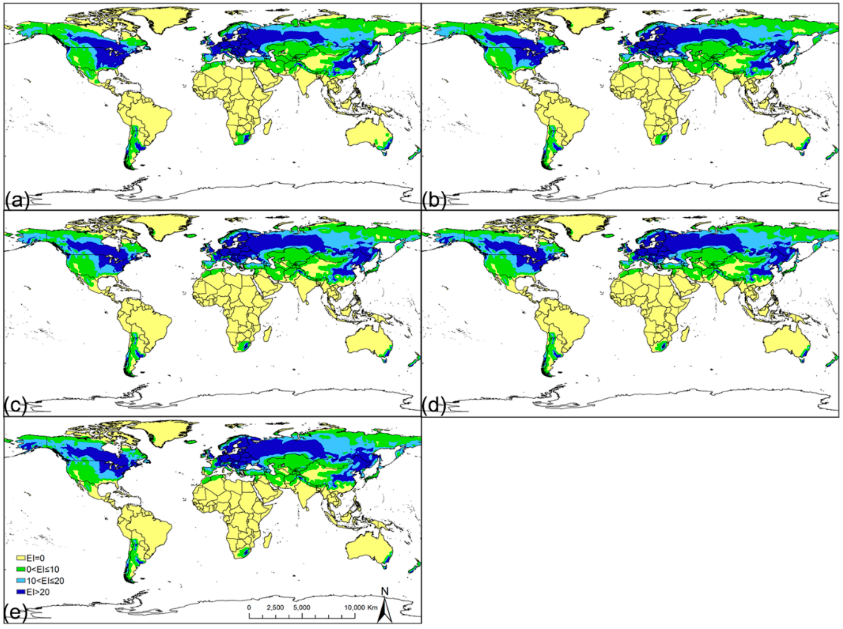
3.2. Potential Distribution under Historical Climate Conditions

The potential distribution of C. lapathi under historical climate conditions is shown in Figure 2a. The areas of the potential distribution (expressed as percentages) for the pest in each suitable region under historical climate conditions are shown in Figure 3. C. lapathi had a wide climatically suitable distribution, covering 73.43 × 10⁶ km2, or 49.29% of the total land area in the world (excluding Antarctica). The potential distribution of the pest mainly included North America, Africa, Europe, and Asia.
The area of the very favorable region covered 21.83 × 10⁶ km2, which accounts for 14.65% of the total land area. The very favorable region was mainly located in North America, Europe, and Asia, including Southern Canada, Eastern United States, China, Central and Eastern Argentina, and most regions of Europe and Western Russia. The area of the favorable region was 18.93 × 10⁶ km2, which accounts for 12.70% of the total land area in the world. The favorable region was mainly located in North America and Asia, with small areas in Europe, Africa, and Oceania. The favorable region included Southern Canada, Central United States, large parts of Russia, and Eastern China. The area of suitable region was 32.68 × 10⁶ km2, which accounts for 21.93% of the total land area. The suitable region was mainly located in North America, Africa, and Asia, including large parts of Alaska, Argentina, Kazakhstan, Uzbekistan, Japan, Iran, Western Canada, United States, and Northeastern Russia.

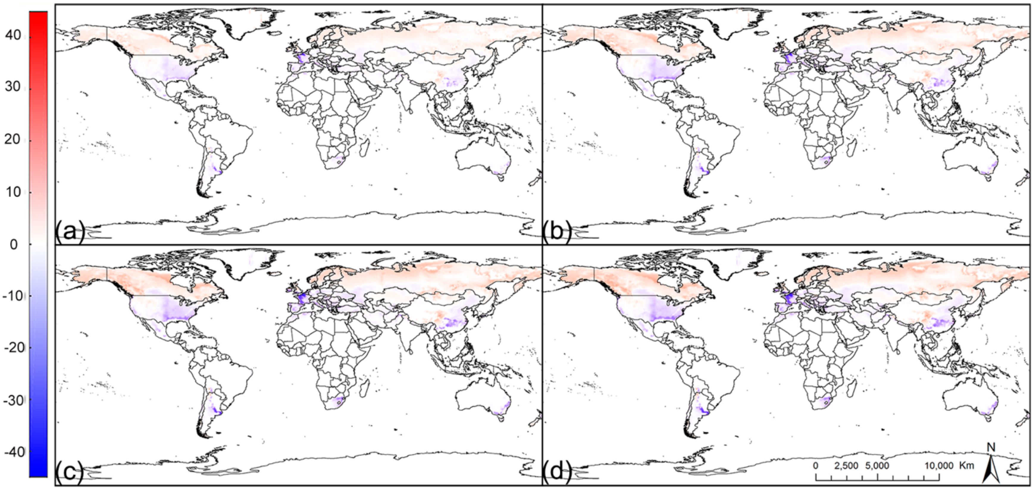
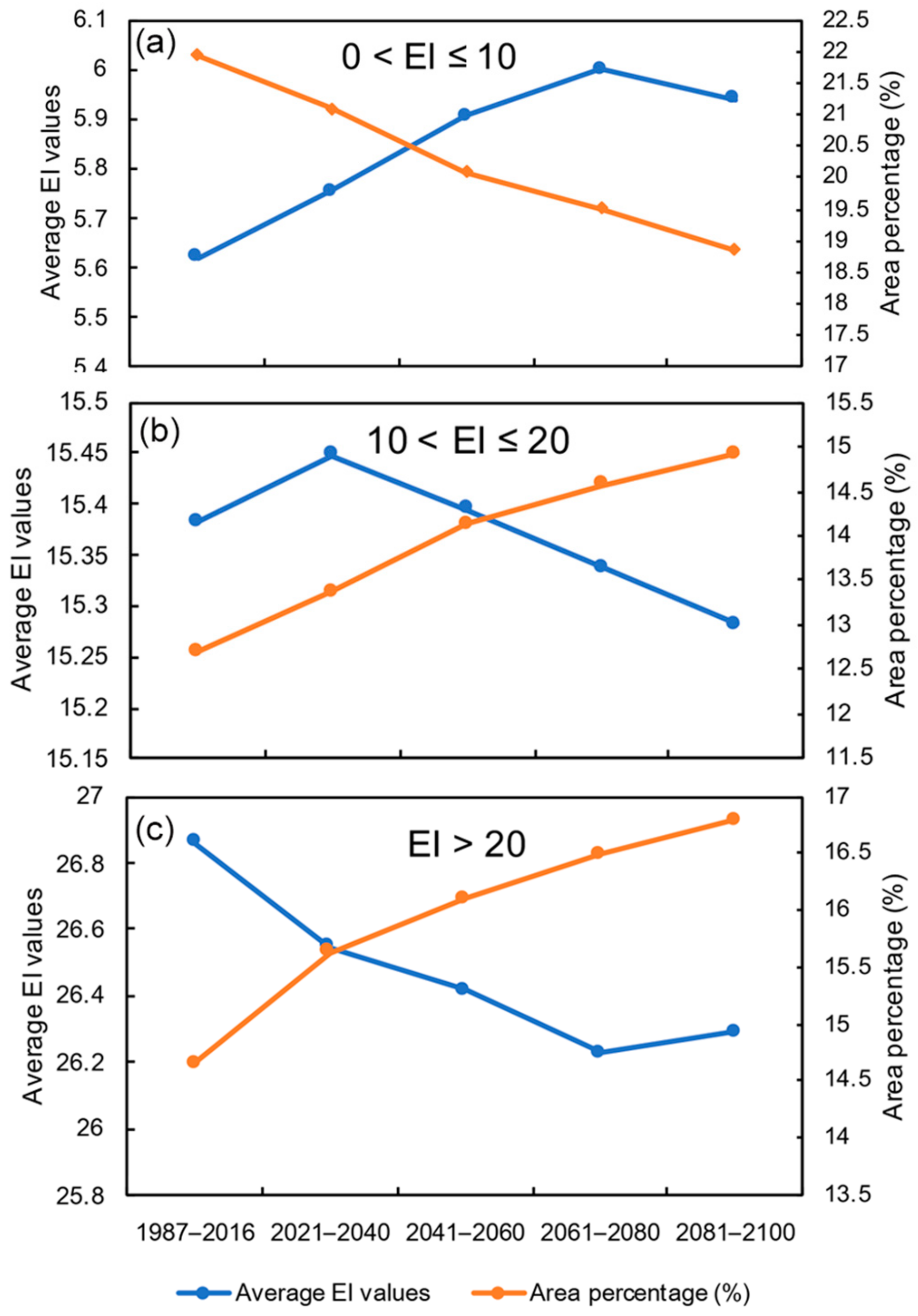
3.3. Potential Distribution under Future Climate Conditions

The potential distribution of C. lapathi under future climate conditions is shown in Figure 2b–e. In general, the climatically suitable regions would move northward, from 74 °N to 76 °N by 2081–2100. Some very favorable regions would shift to a favorable region, and some favorable regions would become very favorable. The potential distribution (expressed as percentages) for the pest on each suitable range under future climate conditions are shown in Figure 3. The total suitable areas would increase by 2080–2100. The impacts of climate change on the climatic suitability of the pest are shown in Figure 4. Climatic suitability would clearly change in large regions of the northern hemisphere and decrease in a small region of the southern hemisphere. The average EI values would change slightly in the future (Figure 3).
Under future climate conditions, the northern boundary of the C. lapathi region was predicted to move northward, and the range of the unsuitable region in the northern hemisphere would gradually decrease. Regarding a very favorable region, the northern boundary would change from 66 °N to 70 °N by 2080–2100. Some very favorable region in Eastern United States, Eastern Argentina, and China would gradually become favorable in the future. For a favorable region, the northern boundary would change from 70 °N to 72 °N by 2080–2100. Some favorable region in Alaska and Western Russia would become very favorable. The range of the suitable region may gradually extend in the northern direction. Some suitable regions in Canada and Northern Russia would become favorable, and some suitable regions in Eastern Australia and Lesotho would become unsuitable.
The total suitable area would increase 1.90 × 10⁶ km2 by 2080–2100, which corresponds to 1.28% of the total land area. In particular, areas of very favorable and favorable regions were predicted to increase by 2.14% and 2.21%, respectively, while the area of the suitable region may decrease by 3.08%. The areas of favorable and very favorable regions were predicted to change in a similar way, with gradual increases by the end of the century. A suitable region would gradually decrease by the end of the century.
We calculated average EI values for regions differing in favourability (Figure 4). The average EI values for a very favorable region were projected to gradually decrease until 2061–2080 and then increase slightly until 2081–2100. Lastly, the average EI values for a very favorable region would decrease by 0.57. The average EI values for a favorable region would first increase until 2021–2040 and then decrease until 2081–2100. Lastly, the average EI values for a favorable region would decrease by 0.10. A suitable region may first clearly increase and then decrease slightly. The average EI values for the suitable region would increase by 0.32. The climatic suitability of the pest would clearly increase in large parts of Alaska, Canada, Norway, Sweden, Finland, Russia, and Central China. Moreover, the climatic suitability of the pest would decrease in Eastern United States, Argentina, Lesotho, Southeastern China, and large regions of Europe.
In a comparison of the climatic suitability between historical and future climate conditions, we found that the areas in which climatic suitability increases were larger than those in which suitability decreases, especially in North America and Asia. Additionally, the total suitable area would increase by the end of the century. These results showed that large areas are at high risk of invasion by the pest under climate change.

3.4. Indices Limiting the Potential Distribution

In the underlying CLIMEX model, we can see that a GI value of 0 or an SI value greater than 100 results in an EI value of 0, which indirectly limits the survival of C. lapathi. In addition, if diapause cannot be successfully completed in the target area (DI = 0), an EI value of 0 can be obtained. Based on these principles and the output value for each index, the CLIMEX model results suggested that the potential distribution of C. lapathi is limited by GI (TI, MI), DI, DS, HS, and WS (CS was not set in this study).
We explored how single indices and interactions among multiple indices affect the potential distribution of C. lapathi. The conditions that limited the potential distribution of C. lapathi are listed in Table 3. It should be noted that GI limits the potential distribution of C. lapathi in two ways. In one case, the distribution is limited by humidity (MI = 0) alone. In another case, it is limited by the interaction of temperature and humidity (TI ≠ 0 and MI ≠ 0). In this case, there are some months when the temperature is suitable and the humidity is not suitable or the humidity is suitable and the temperature is not suitable, which results in an EI value of 0, expressed by GI′.
With future climate change, areas limited by HS and HS interaction indices may increase significantly and areas limited by DI and DI interaction indices may decrease significantly. Under historical climate conditions, 18 factors limited the potential distributions. From 2021 to the 2100s, the combination of DI, HS, and TI will be another factor. From the 2061s, MI+TI+DI will no longer be a limiting factor. From 1987 to the 2080s, regions limited by HS, DI+HS, DI+HS+TI, DI+HS+GI′, DI+HS+MI, and DI+HS+DS+MI will gradually increase. Regions limited by MI, GI′, DI+GI′, DI+TI, DI+MI, and DI+TI+MI will gradually decrease. Regions limited by the remaining factors do not change substantially. DI and DI+GI′ are dominant factors that limit the widest range of potential distribution. DI+GI’ is a limiting factor for all continents except Antarctica. The specific regions limited by each index are listed in Table 3 and mapped in Figure 5.

4. Discussion

This study reveals that C. lapathi has a potentially wide distribution range in many climatically suitable regions throughout the world, mainly in North America, Europe, and Asia, under historical climate conditions. We predict that climatically suitable regions will move northward and total suitable areas will increase under historical climate conditions. We compared our results with those of Ji (2015) [13], which showed that the projected potential distribution in China differs between the two studies, likely due to differences in the data and models used. Using CLIMEX, GARP, and MaxEnt, Ji (2015) [13] predicted different potential distributions of C. lapathi in China from those obtained in our study, possibly due to differences in climate data, CLIMEX parameters, and models. Ji (2015) [13], using CLIMEX, predicted a wider potential distribution in Northwestern and Southern China between 1961 and 2000. We also predicted the historical potential distribution between 1987 and 2016. The CLIMEX parameters used in our study differ from those used by Ji (2015) [13], with respect to pest distribution data and the version of CLIMEX. In addition, the different algorithms used in the three models will result in different predictions.
A large number of emerging robust modeling approaches that can explain the dynamic range of species habitats and predict the impact of climate change on distribution have become one of the most widely researched topics in applied ecology, evolutionary ecology, and biogeography [32,33]. Given that a large and steadily increasing number of species distribution models (SDMs) have been developed, how to select the appropriate methodology based on their needs is becoming a challenge, especially for the uninitiated [34,35,36]. Generally, SDMs include mechanistic and correlative approaches [37]. Mechanistic models explicitly incorporate physiologically constraining methods that convey a species’ tolerance to environmental conditions [33,37]. These mechanistic models require a detailed understanding of physiological processes, which makes it difficult to develop for all but the most well-understood species. Correlative models assume current distribution gives a good indicator of ecological requirements by relating occurrence records to spatial environmental data [37,38]. The central premise of this approach is that the observed distribution of a species provides useful information for the environmental requirements of that species [37]. Due to the flexibility of their data requirements and ease of use, correlative approaches are more practical over mechanistic approaches [39,40]. Lantschner et al. [41] compared modelling tools in terms of correlative or mechanistic approaches from 220 publications and found that semi-mechanistic approaches were the most frequently used ones (56% of the articles). With a thorough understanding of their advantages and limitations, we thought that CLIMEX, as a semi-mechanistic approach, was more suitable for exploring the potential impact of climate change on the potential distribution of C. lapathi based on the availability of the model, biological data of the pest, and the appropriate model validation.
Uncertainty in climate models and natural variability within climate systems may result in uncertainty in climate prediction, which will influence the predicted results [42]. In addition to climate change, other factors, including topography, soil type, host plant availability, land use, and human impact, may also limit the potential distribution of pests [18]. Insects rely on the nutrition and space provided by host plants for survival. Accordingly, the distribution of host plants will limit the distribution of insects. However, C. lapathi can feed and reproduce on a large number of Populus and Salix species, which have large global distributions [4]. Pests may shift to new host plants when they invade new regions. Thus, host plants were not considered in this study. In fact, biological properties of species differ among regions, but uniform parameters are typically used in studies, which affects the accuracy of projections [43]. Biological characteristics of species would also exhibit evolutionary changes over time, and these changes may impact the projected distributions. Climate is the only tractable factor for obtaining an initial and conservative estimate of the potential distribution of species [18]. Our study still exists an uncertainty due to the limited approach since the predictions only rely on CLIMEX. With the development of species distribution models, it is recommended that projections of future assessments consider additional non-climatic factors and incorporate other SDMs’ predictions to better manage the invasion risk and strengthen the accuracy of predictions [44].
Using the Köppen-Geiger climate classification [45], we attempted to verify and explain the reasons for the indices by limiting potential distribution. The climates in areas limited by HS and HS interaction indices are mainly in Group B, Dry (arid and semiarid) climates, including the Warm desert climate (BWh) and the Warm semi-arid climate (BSh). This type of climate is characterized by little precipitation. Therefore, precipitation may be one reason why these regions will become unsuitable regions. Increases in global temperature are accompanied by increases in precipitation, which may satisfy moisture demand and remove the HS restriction. In the DI and DI interaction indices, the factor that limits the maximum extent of the area is DI and DI+GI′. The scope of the DI limited area is not clear under future climate conditions, and, hence, will not be considered. In areas restricted by DI+GI′, climates mostly belong to Group C (temperate climates), which have average temperatures in the coldest month between 0 °C (or −3 °C) and 18 °C and at least one month with an average temperature above 10 °C [46]. The main reason for these regional restrictions may be that winter temperatures are too low to break diapause or are insufficient for thermal accumulation during the growth season to enable the species to complete a minimum amount of development. In view of global warming, the limitation will gradually be overcome.
Attention has to be paid to the prevention and control of C. lapathi. Climate change has a significant influence on the spread of C. lapathi. Thus, our maps of its potential distribution could help identify areas that are at risk of pest invasion in the future. Given that the spread of C. lapathi is mainly dependent on the artificial transfer of seedlings or newly harvested nursery stock harboring overwintering eggs or newly hatched larvae, inspection and quarantine work performed in advance in these newly transformed regions will be of great significance for minimizing risks. For areas expected to change gradually from suitable to unsuitable, the effectiveness of prevention and control approaches could be gradually reduced, and governments could shift their efforts to reduce unnecessary financial losses. For areas that are consistently very favorable in the future, a comprehensive prevention strategy is necessary. Since adults move quickly and larvae drill in the bark (early instars) and xylem (later instars), it is difficult to adopt practical and efficient insecticide control tactics against either the larval or adult stage of C. lapathi [9,24]. Drilling injection is effective for the control of C. lapathi, with an efficiency of up to 89.85% [47]. Physical barriers applied to the stem also effectively impede the movement and oviposition of C. lapathi [48]. In terms of biological control, natural enemies and microorganisms, such as woodpeckers, Beauveria brongniartii (Sacc.), and Scleroderma guani, are adopted to control pests [49,50]. In addition, damage caused by C. lapathi varies among hybrid poplar clones [9]. Under the premise that resistant clones adapt to the ecological environment of the planting area, growers should choose less susceptible varieties to prevent larval development, likely in the early spring [9]. The antennae of C. lapathi showed consistent strong responses to (E)-conophthorin, which was discovered in the stem volatiles of willow, suggest that conophthorin may be behaviorally important in the pest, and may be used to control the pest [51]. Furthermore, in a behavioral response test, furfural (a host plant volatile) showed a significantly higher luring effect on female adults of C.lapathi, and the luring rate was 71.59%. Nerol (a non-host plant volatile) and benzoic acid (a host plant volatile) showed a significantly higher repelling effect on female adults of C.lapathi. The repelling rates were up to 81.5% and 74.68%, respectively. Male adults of C.lapathi were significantly repelled by cedar oil (a non-host plant volatile) and the repelling rate was 78.75%. These plant volatiles could be of great importance to the biological control of the pest [52]. Developing strategies for pest management rely on obtaining accurate information on occurrence, particularly the onset and peak periods of occurrence. Global climate warming will increase both insect population growth and the insect metabolic rate. Hence, the prevention and control strategies should be adjusted to take into account changes in occurrence. Recently, changes in the relationships between trophic levels brought about by changes in the phenology of interacting species have been observed. This has been confirmed for eastern spruce budworm (Choristoneura fumiferana) and its host trees [53,54,55]. The precise impacts of climate change on phenological synchrony between C. lapathi, natural enemies, and host plants still remain somewhat uncertain. Long–term studies are, therefore, required to determine how climate change will alter biology and ecology. Long–term integrated pest management approaches will be essential to minimize further losses by C. lapathi.

5. Conclusions

Climatic suitability would clearly change in large regions of the northern hemisphere and decrease in a small region of the southern hemisphere. The areas in which climatic suitability increases would be larger than those in which suitability decreases, especially in North America and Asia. Moreover, the total suitable area would increase by the end of the century. According to the changes in potential distribution, the effectiveness of prevention and control approaches for newly unsuitable distribution could be gradually reduced, and inspection and quarantine work performed in advance in these newly transformed habitats will be of great significance in minimizing risks. The findings will provide a reference for the effective control of expanding pest populations, and lay the foundation for further study of the mechanisms underlying the responses of C. lapathi to global climate change.

Author Contributions

Conceptualization, X.G. and S.Z. Data curation, Y.Z. and L.Z., L.C. and T.W. Formal analysis, Y.Z., L.Z., X.L., and X.G. Funding acquisition, S.Z. Investigation, L.Z. Methodology, Y.Z., L.Z., X.G., and S.Z. Project administration, X.G. and S.Z. Resources, T.W. Software, L.Z. and S.G. Supervision, X.G. and S.Z. Validation, Y.Z. and X.G. Writing—original draft, Y.Z. and L.Z. Writing—review and editing, X.G. and S.Z. All authors have read and agreed to the published version of the manuscript.

Funding

The Fundamental Research Funds for the Central Universities (NO. 2016ZCQ07) supported this study.

Conflicts of Interest

The authors declare no conflict of interest.

References

  1. Broberg, C.L.; Borden, J.H.; Humble, L.M. Distribution and abundance of Cryptorhynchus lapathi on Salix spp. Can. J. For. Res. 2002, 32, 561–568. [Google Scholar] [CrossRef]
  2. Schoene, W.J. The Poplar and Willow Borer (Cryptorhynchus lapathi L.); New York Agricultural Experiment Station: Geneva, NY, USA, 1907; Volume 286, pp. 83–104. [Google Scholar]
  3. Harris, J.W.E.; Coppel, H.C. The poplar-and-willow borer, Sternochetus (=Cryptorhynchus) lapathi (Coleoptera: Curculionidae), in British Columbia. Can. Entomol. 1967, 99, 411–418. [Google Scholar] [CrossRef]
  4. CABI, Cryptorhynchus lapathi (Poplar and Willow Borer). Available online: https://www.cabi.org/cpc/datasheet/16433 (accessed on 13 November 2018).
  5. Qin, P.C.; Yao, F.M.; Cao, X.X.; Zhang, J.H.; Cao, Q. Development process of modeling impacts of climate change on agricultural productivity based on crop models. Chin. J. Agrometeorol. 2011, 32, 240–245. [Google Scholar]
  6. Jia, J. Risk Aanalysis on Cryptorrhynchus lapathi in Qinghai. Sci. and Technol. of Qinghai Agriculture and For. 2015, 2, 29–31. [Google Scholar]
  7. Fang, S.Y. Preliminary study on poplar weevil. Sci. Silvae Sin. 1964, 10, 81–85. [Google Scholar]
  8. Jodal, I. A study of the susceptibility of poplar clones to the attack of poplar and willow borer (Cryptorhynchus lapathi). Radovi Institut za Topolarstvo (Yugoslavia) 1987, 1, 95–108. [Google Scholar]
  9. Broberg, C.L.; Borden, J.H.; Gries, R. Olfactory and feeding preferences of Cryptorhynchus lapathi L. (Coleoptera: Curculionidae) among hybrid clones and natural poplars. Environ. Entomol. 2005, 34, 1606–1613. [Google Scholar] [CrossRef] [Green Version]
  10. Li, Y.J.; Zhong, Z.K.; Lin, J.H.; Qu, P. Bionomics and control of poplar weevil. Acta Entomol. Sin. 1981, 24, 390–396. [Google Scholar]
  11. Smith, B.D.; Stott, K.G. The life history and behaviour of the willow weevil Cryptorrhynchus lapathi L. Ann. Appl. Biol. 2010, 54, 141–151. [Google Scholar] [CrossRef]
  12. Gao, R.T.; Qin, X.X.; Chen, H.D.; Sun, Y.Q. Preliminary study on susceptibility of poplar varieties to Cryptorrhynchus lapathi (L.). For. Pest Dis. 1987, 3, 16–18. [Google Scholar]
  13. Ji, Y.C. Study on Suitable Area and Economic Loss Assessment of Ten Important Forestry Weevils in China. Master’s Thesis, Shandong Agricultural University, Shandong, China, 2015. [Google Scholar]
  14. Shen, G. Research of Farming Information Investigation Platform. Master’s Thesis, North China Electric Power University, Beijing, China, 2015. [Google Scholar]
  15. IPCC. Climate Change 2013: The Physical Scientific Basis. Contribution of Working Group? To the Fifth Assessment Report of the Intergovernmental; Cambridge University Press: Cambridge, UK; New York, NY, USA, 2013. [Google Scholar]
  16. Chen, Y. Effect of global warming on insect: A literature review. Acta Ecol. Sin. 2010, 30, 2159–2172. [Google Scholar]
  17. Liu, E. Studies on Early-Warming Techniques and Risk Assessment for the Poplar Stem Boring Pests in Heilongjiang Province. Master’s Thesis, Northeast Forestry University, Harbin, China, 2009. [Google Scholar]
  18. Kriticos, D.J.; Maywald, G.F.; Yonow, T.; Zurcher, E.J.; Herrmann, N.I.; Sutherst, R. Exploring the Effects of Climate on Plants, Animals and Diseases; CLIMEX Version; CSIRO: Canberra, Australia, 2015; Volume 4, p. 184. [Google Scholar]
  19. Sutherst, R.W.; Maywald, G.F.; Kriticos, D.J. CLIMEX Version 3: User’s Guide; Hearne Scientific Software: Melbourne, Australia, 2007. [Google Scholar]
  20. Cui, Y.; Wei, F.; Zhu, Z.; Wang, X.; Peng, D.; Xie, B. Potential distribution of Diaporthe phaseolorum var. caulivora in China by using CLIMEX and GIS tools. Plant Prot. 2009, 35, 49–53. [Google Scholar]
  21. Harris, I.C.; Jones, P.D. CRU TS4. 01: Climatic Research Unit (CRU) Time-Series (TS) Version 4.01 of High-Resolution Gridded Data of Month-by-Month Variation in Climate (Jan. 1901-Dec. 2016); Centre for Environmental Data Analysis: Chilton, UK, 2017; Volume 4. [Google Scholar]
  22. Zou, Y.; Ge, X.; Guo, S.; Zhou, Y.; Wang, T.; Zong, S. Impacts of climate change and host plant availability on the global distribution of Brontispa longissima (Coleoptera: Chrysomelidae). Pest Manag. Sci. 2019, 76, 244–256. [Google Scholar] [CrossRef] [PubMed]
  23. Garbutt, R.; Harris, J.W.E. Poplar and Willow Borer; Pest Leaflet—Pacific Forest Centre Forestry: Victoria, BC, Canada, 2002. [Google Scholar]
  24. Hannon, E.; Kittelson, N.; Eaton, J.; Brown, J. Screening hybrid poplar clones for susceptibility to Cryptorhynchus lapathi (Coleoptera: Curculionidae). J. Econ. Entomol. 2008, 101, 199–205. [Google Scholar] [CrossRef]
  25. Yu, X.Y.; Du, Y.D. Report and control of Cryptorrhynchus lapathi (L.). J. Heilongjiang For. 1997, 12–13. [Google Scholar]
  26. Doom, D. The biology, damage and control of the poplar and willow borer, Cryptorrhynchus lapathi. Neth. J. Plant Pathol. 1966, 72, 233–240. [Google Scholar] [CrossRef]
  27. Jin, D.; Lue, L.; Li, L. Status and Perspective of Research on Cryptorrhynchus lapathi in China. J. Northeast For. Univ. 2003, 31, 75–77. [Google Scholar] [CrossRef]
  28. Dong, Q.Y. Investigation of Cryptorrhynchus lapathi (L.) hazard to several poplar species. For. Invest. Des. 2004, 41–42. [Google Scholar]
  29. Li, X.E.; Shen, Z.A.; Zhu, H. Bionomics and Control of Cryptorrhynchus lapathi (L.); China Association for Science and Technology: Wuhan, China, 2007. [Google Scholar]
  30. Niu, H.X. Forest quarantine insect pest, Cryptorrhynchus lapathi L. in Hebei Province. J. Hebei. For. Sci. Technol. 1984, 28–29. [Google Scholar]
  31. Geier, P.W. The life history of Codling Moth, Cydia pomonella (L.) (Lepidoptera: Tortricidae), in the Australian Capital Territory. Aust. J. Zool. 1963, 11, 323–367. [Google Scholar] [CrossRef]
  32. Araújo, M.B.; Peterson, A.T. Uses and misuses of bioclimatic envelope modeling. Ecology 2012, 93, 1527–1539. [Google Scholar] [CrossRef] [PubMed] [Green Version]
  33. Kearney, M.; Porter, W. Mechanistic niche modelling: Combining physiological and spatial data to predict species’ ranges. Ecol. Lett. 2009, 12, 334–350. [Google Scholar] [CrossRef] [PubMed]
  34. Elith, J.H.; Graham, C.P.; Anderson, R. Novel methods improve prediction of species’ distributions from occurrence data. Ecography 2006, 29, 129–151. [Google Scholar] [CrossRef] [Green Version]
  35. Thuiller, W.; Lafourcade, B.; Engler, R.; Araújo, M.B. BIOMOD—A platform for ensemble forecasting of species distributions. Ecography 2009, 32, 369–373. [Google Scholar] [CrossRef]
  36. Heikkinen, R.K.; Luoto, M.; Araújo, M.B.; Virkkala, R.; Thuiller, W.; Sykes, M. Methods and uncertainties in bioclimatic envelope modelling under climate change. Prog. Phys. Geogr. 2006, 30, 751–777. [Google Scholar] [CrossRef] [Green Version]
  37. Pearson, R.G. Species’ distribution modeling for conservation educators and practitioners. Synth. Am. Mus. Nat. Hist. 2007, 50, 54–89. [Google Scholar]
  38. Kearney, M.R.; Wintle, B.A.; Porter, W.P. Correlative and mechanistic models of species distribution provide congruent forecasts under climate change. Conserv. Lett. 2010, 3, 203–213. [Google Scholar] [CrossRef]
  39. Magarey, R.; Newton, L.; Hong, S.C.; Takeuchi, Y.; Christie, D.; Jarnevich, C.S.; Castro, K. Comparison of four modeling tools for the prediction of potential distribution for non-indigenous weeds in the United States. Biol. Invasions 2018, 20, 679–694. [Google Scholar] [CrossRef]
  40. Moilanen, A.; Wintle, B.A. Quantitative reserve network aggregation via the boundary quality penalty. Conserv. Biol. 2007, 21, 355–364. [Google Scholar] [CrossRef]
  41. Lantschner, M.V.; de la Vega, G.; Corley, J.C. Predicting the distribution of harmful species and their natural enemies in agricultural, livestock and forestry systems: An overview. Int. J. Pest Manage. 2019, 65, 190–206. [Google Scholar] [CrossRef]
  42. Hawkins, E.; Sutton, R. The potential to narrow uncertainty in regional climate predictions. Bull. Am. Meteorol. Soc. 2009, 90, 333–337. [Google Scholar] [CrossRef] [Green Version]
  43. Ge, X.; He, S.; Zhu, C.; Wang, T.; Xu, Z.; Zong, S. Projecting the current and future potential global distribution of Hyphantria cunea (Lepidoptera: Arctiidae) using CLIMEX. Pest Manag. Sci. 2019, 75, 160–169. [Google Scholar] [CrossRef] [PubMed] [Green Version]
  44. Aljaryian, R.; Kumar, L. Changing global risk of invading greenbug Schizaphis graminum under climate change. Crop Prot. 2016, 88, 137–148. [Google Scholar] [CrossRef]
  45. Beck, H.E.; Zimmermann, N.E.; McVicar, T.R.; Vergopolan, N.; Berg, A.; Wood, E.F. Present and future Köppen-Geiger climate classification maps at 1-km resolution. Sci. Data 2018, 5, 180214. [Google Scholar] [CrossRef] [Green Version]
  46. Peel, M.C.; Finlayson, B.L.; Mcmahon, T.A. Updated world map of the Köppen-Geiger climate classification. Hydrol. Earth Syst. Sci. 2007, 11, 259–263. [Google Scholar] [CrossRef] [Green Version]
  47. Lei, Y.U. Effect analysis of drilling injection against Cryptorrhynchus lapathi. Biol. Disaster Sci. 2017, 40, 181–184. [Google Scholar]
  48. Allegro, G. Mechanical control of the principal xylophagous insects of poplar using trunk barriers (In Italian). Inform. Agr 1990, 46, 91–95. [Google Scholar]
  49. Cao, Q.J.; Chi, D.F.; Yu, J.; Ran, Y.L. SEM and TEM observations of Beauveria brongniartii (Sacc.) Petch infecting body wall of Cryptorhynchus lapathi L. (Coleoptera: Curculionidae) larvae. J. Beijing For. Univ. 2015, 37, 96–101. [Google Scholar]
  50. Li, Y.X. The life habit and characteristics of Scleroderma guani Xiao et Wu. Gansu. Agric. 2014, 14, 72–73. [Google Scholar] [CrossRef]
  51. Broberg, C.; Borden, J.; Gries, R. Antennae of Cryptorhynchus lapathi (Coleoptera: Curculionidae) detect two pheromone components of coniferophagous bark beetles in the stems of Salix sitchensis and Salix scouleriana (Salicaceae). Can. Entomol. 2005, 137, 716–718. [Google Scholar] [CrossRef]
  52. Xing, Y.; Chi, D.; Yu, J.; Yan, J.; Ran, Y. EAG and behavioral responses of Cryptorrhynchus lapathi (Coleoptera: Curculionidae) to Twelve Plant Volatiles. Sci. Silvae Sin. 2017, 53, 159–167. [Google Scholar]
  53. Pureswaran, D.S.; Neau, M.; Marchand, M.; Grandpré, L.D.; Kneeshaw, D. Phenological synchrony between eastern spruce budworm and its host trees increases with warmer temperatures in the boreal forest. Ecol. Evol. 2018, 9, 576–586. [Google Scholar] [CrossRef] [PubMed]
  54. Kocmánková, E.; Trnka, M.; Juroch, J.; Dubrovský, M.; Semerádová, D.; MožNý, M.; Žalud, Z.; Pokorný, R.; Lebeda, A. Impact of climate change on the occurrence and activity of harmful organisms. Plant Prot. Sci. 2009, 45, S48–S52. [Google Scholar] [CrossRef] [Green Version]
  55. Forrest, J.R. Complex responses of insect phenology to climate change. Curr. Opin. Insect Sci. 2016, 17, 49–54. [Google Scholar] [CrossRef] [PubMed]
Figure 1. Current global distribution of C. lapathi. (a) Data sources. Red dots represent distribution records in GBIF and grey shadows indicate distribution records in CABI and references. (b) Blue triangles and blue shadows indicate regions that were selected for modelling, and green triangles and green shadows indicate regions that were selected for validation.
Forests 11 00005 g001
Figure 2. Global potential distribution of C. lapathi under historical and future climate conditions. (a) Global potential distribution for C. lapathi under historical climate conditions (1987−2016). (be) show the global potential distribution for C. lapathi in the 2030s (2021–2040), 2050s (2041–2060), 2070s (2061–2080) and 2090s (2081–2100). Yellow regions indicate unsuitable regions (EI = 0), green regions indicate suitable regions (0 < EI ≤ 10), blue regions indicate favorable regions (10 < EI ≤ 20), and dark blue regions indicate very favorable regions (EI > 20).
Forests 11 00005 g002
Figure 3. Changes in Ecoclimatic Index (EI) values under historical (1987–2016) and future (2021–2040, 2041–2060, 2061–2080, and 2081–2100) climate conditions. Red represents an increase, blue represents a decrease, and the depth of colour indicates the degree of change in EI values. (a) 1987–2016, (b) 2021–2040, (c) 2041–2060, (d) 2061–2080, and (e) 2081–2100.
Forests 11 00005 g003
Figure 4. Changes in average Ecoclimatic Index (EI) values and potential distribution areas for C. lapathi with differing climate favorabilities between historical climate conditions (1987–2016) and future climate conditions (2021–2040, 2041–2060, 2061–2080, and 2081–2100). (a) Changes in average EI values and the area of potential distribution for C. lapathi in suitable regions (0 < EI ≤ 10). (b) Changes in average EI values and area of potential distribution for C. lapathi in favorable regions (10 < EI ≤ 20). (c) Changes in average EI values and area of potential distribution for C. lapathi in very favorable regions (EI > 20). Blue line indicates the change in favourability. The orange line indicates the change in area (as a percentage).
Forests 11 00005 g004
Figure 5. Distribution maps for five different conditions. (a) 1987–2016, (b) 2021–2040, (c) 2041–2060, (d) 2061–2080, and (e) 2081–2100. MI-Moisture Index, GI-Growth Index, DI-Diapause Index, HS-Heat Stress, WS-Wet Stress, TI-Temperature Index, MI-Moisture Index, and DS-Dry Stress.
Forests 11 00005 g005
Table 1. CLIMEX parameter values for Cryptorhynchus lapathi (L.).
CLIMEX ParameterSemi-Arid TemplateFacultative Diapause TemplateTemperate TemplateFinal ParameterUnits
DV0-Lower Temperature Threshold10888°C
DV1-Lower Optimum Temperature20181816°C
DV2-Upper Optimum Temperature32262420°C
DV3-Upper Temperature Threshold38312836°C
PDD-Length of growing season00600/DD
DPD0-Diapause Induction Daylength/11/11DD
DPT0-Diapause Induction Temperature/5/10°C
DPT1-Diapause Termination Temperature/0/4°C
DPD-Diapause Development Days/90/90DD
DPSW-Diapause Summer or Winter indicator/0/0
TTCS-Cold Stress Temperature Threshold0/00°C
THCS-Cold Stress Temperature Rate0/00week−1
TTHS-Heat Stress Temperature Threshold39/3036°C
THHS-Heat Stress Temperature Rate0.002/0.0050.005week−1
SM0-Lower Soil Moisture Threshold0.10.30.250.1
SM1-Lower Optimal Soil Moisture0.20.70.80.3
SM2-Upper Optimal Soil Moisture0.2511.51
SM3-Upper Soil Moisture Threshold0.322.51.5
SMDS-Dry Stress Threshold0.05/0.20.01
HDS-Dry Stress Rate−0.005/−0.005−0.005week−1
SMWS-Wet Stress Threshold0.4/2.51.5
HWS-Wet Stress Rate0.01/0.0020.002week−1
Table 2. Parameter sensitivity analysis for Cryptorhynchus lapathi (L.).
ParameterLowDefaultHighRange Change
1987–20162021–20402041–20602061–20802081–2100
SM000.10.23.83.43.22.92.8
SM10.20.30.40.60.50.40.40.4
SM20.911.100000
SM31.41.51.600000
DV078900000
DV11516170.10.10.10.10.1
DV219202100000
DV335363700000
DPD010.51111.50.50.40.40.30.3
DPT0910110.10.10.10.10.1
DPT13454.23.93.63.43.3
DPD72901080.50.40.40.40.4
TTCS−24−23−2200000
THCS−0.012−0.01−0.00800000
TTHS3536370.20.30.30.30.3
THHS0.0040.0050.00600.10.10.10.1
SMDS00.10.20.20.20.10.10.1
HDS−0.006−0.005-0.00400000
SMWS1.41.51.600000
HWS0.00160.0020.002400000
SM0-Lower soil moisture threshold, SM1-Lower optimal soil moisture, SM2-Upper optimal soil moisture, SM3-Upper soil moisture threshold, DV0-Lower temperature threshold, DV1-Lower optimum temperature, DV2-Upper optimum temperature, DV3-Upper temperature threshold, DPD0-Diapause induction daylength, DPT0-Diapause induction temperature, DPT1-Diapause termination temperature, DPD-Diapause development days, TTCS-Cold stress temperature threshold, THCS-Cold stress temperature rate, TTHS-Heat stress temperature threshold, THHS-Heat stress temperature rate, SMDS-Dry stress threshold, HDS-Dry stress rate, SMWS-Wet stress threshold, and HWS-Wet stress rate.
Table 3. Indices limiting the potential distribution.
IndexLegendRegions Limited by IndicesChange of Range
MI
(Moisture Index)
MI = 0Northwest China, the Western United States, Chile, Argentina, South Africa, and New ZealandThe limited regions in Western United States will gradually decrease
GI′
(combination of Growth Index, Temperature Index, and Moisture Index)
GI′ = 0
(GI = 0, TI ≠ 0, MI ≠ 0)
Western United States, Central Asia, and scattered areas of Northwest ChinaThe limited regions in central Asia will gradually decrease
DI
(Diapause Index)
DI = 030°S and 30°N at low latitudesChange is not clear
HS
(Heat Stress)
HS ≥ 100Central Asia and the scattered areas of the Southern United StatesThe limited regions in central Asian will gradually expand northward to 40°N
DI+HS
(Diapause Index + Heat Stress)
DI = 0, HS ≥ 1005°N-15°N in Africa, India, Mexico, Brazil, sporadic regions of VenezuelaThe limited regions in India will gradually increase
DI+GI′
(Diapause Index + combination of Growth Index, Temperature Index and Moisture Index)
DI = 0, GI′ = 0
(DI = 0, GI = 0, TI ≠ 0, MI ≠ 0)
20°S-45°S, 20°N -40°N, Western Europe, Canada, and Northern RussiaOverall decrease
DI+TI
(Diapause Index + Temperature Index)
DI = 0, TI = 0Arctic Circle and Western ChinaThe limited regions in China will gradually increase
DI+MI
(Diapause Index + Moisture Index)
DI = 0, TI = 0North and South Africa, Arabia, and South AustraliaThe limited regions in China and Africa will gradually decrease
HS+GI′
(Heat Stress + combination of Growth Index, Temperature Index and Moisture Index)
HS ≥ 100, GI′ = 0US-Mexico border, Iran’s sporadic regionsChange is not clear
HS + MI
(Heat Stress + Moisture Index)
HS ≥ 100, GI′ = 0Roughly the same as HS+GI′Change is not clear
DI + WS
(Diapause Index + Wet Stress)
DI = 0, WS ≥ 100Sporadic regions of Colombia and IndiaChange is not clear
DI + HS + TI
(Diapause Index + Heat Stress + Temperature Index)
DI = 0, HS ≥ 100, TI = 0Africa, Southern Mexico, and sporadic regions of Iran after 2021The limited regions will gradually expand
DI + TI + MI
(Diapause Index + Temperature Index + Moisture Index)
DI = 0, TI = 0, MI = 080°N and its north of GreenlandThe limited regions will gradually decrease, and it will no longer be a limiting factor after 2061
DI + WS + GI′
(Diapause Index + Wet Stress + combination of Growth Index, Temperature Index and Moisture Index)
DI = 0, WS ≥ 100, GI′ = 0The junction of Panama and ColombiaNo change
DI + WS + MI
(Diapause Index + Wet Stress + Moisture Index)
DI = 0, WS ≥ 100, MI = 0North Western South America and 10°S-5°N area in Southeast AsiaChange is not clear
DI + HS + GI′
(Diapause Index + Heat Stress + combination of Growth Index, Temperature Index and Moisture Index)
DI = 0, HS ≥ 100, GI′ = 010°N-15°N in Africa, Western Mexico, Northern Australia, and sporadic regions along the Arabian Sea coastThe limited regions in Australia will gradually expand southward
DI + HS + MI
(Diapause Index + Heat Stress + Moisture Index)
DI = 0, HS ≥ 100, MI = 015°N-20°N in Africa, Pakistan, the eastern part of the Arabian Peninsula, and sporadic regions in central AustraliaThe limited regions in central Asia and Australia will gradually increase
DI + DS + MI
(Diapause Index + Dry Stress + Moisture Index)
DI = 0, DS ≥ 100, MI = 0Northern Egypt, Southern Arabia, and coastal areas of PeruChange is not clear
DI + HS + DS + MI
(Diapause Index + Heat Stress + Dry Stress + Moisture Index)
DI = 0, HS ≥ 100, DS ≥ 100, MI = 020°N -30°N in Africa and Saudi ArabiaThe limited regions will gradually expand to high latitudes

