Article

Genetic Diversity and Spatial Genetic Structure in Isolated Scots Pine (Pinus sylvestris L.) Populations Native to Eastern and Southern Carpathians

by
Nicolae Șofletea
1,
Georgeta Mihai
2,
Elena Ciocîrlan
1,* and
Alexandru Lucian Curtu
1
1
Faculty of Silviculture and Forest Engineering, Transilvania University of Brasov, 500123 Brasov, Romania
2
National Institute for Research and Development in Forestry “Marin Dracea”, 077190 Voluntari, Romania
*
Author to whom correspondence should be addressed.
Forests 2020, 11(10), 1047; https://doi.org/10.3390/f11101047
Submission received: 14 August 2020 / Revised: 23 September 2020 / Accepted: 25 September 2020 / Published: 28 September 2020
(This article belongs to the Section Forest Ecology and Management)

Abstract

:
Small, isolated populations are more vulnerable to natural disturbances and loss of genetic diversity. Scots pine, an abundant tree species in the boreal forest of Eurasia, has a scattered natural distribution across Eastern and Southern Carpathian Mountains, where only a few relict populations still exist. We estimated genetic diversity and spatial genetic structure in Scots pine on the basis of microsatellite nuclear markers (nSSR) data. We found a relatively high level of genetic diversity (He = 0.697) within populations and no evidence of recent bottlenecks. Genetic diversity was lower in peat bog populations, as compared to populations that grow on rocky slopes or acidic soils and nutrient-poor sites. Population genetic structure was weak, and genetic discontinuities among populations were detected. Spatial genetic structure (SGS) was observed in nearly all Scots pine populations. The strength of SGS, quantified by Sp statistics, varied greatly among populations, ranging from 0.0011 to 0.0207, with an average of 0.01. Our study highlights that Eastern and Southern Carpathian populations still possess high within-population diversity in spite of the recent fragmentation and reduction of the Scots pine natural distribution range. We discuss the importance of spatial patterns of genetic diversity for developing strategies of conservation and sustainable use of Scots pine genetic resources in the Carpathian region.

1. Introduction

Relict forest tree populations, i.e., populations that are presently confined to a small territory, but whose original distribution range was much larger in the past, may contribute substantially to the genetic diversity of a particular species [1]. Geographically isolated populations, which are located at the margins of species distribution range, may harbor rare, unique genetic variants that might be of importance for species survival under changing environmental conditions [2,3]. The genetic diversity of geographically marginal populations, which are typically small and island-like, may be reduced due to higher genetic drift, increased inbreeding, limited or lack of gene flow from other populations, and natural selection after long periods of time of survival in new ecological settings [4,5].
Spatial genetic structure (SGS) within natural tree populations derives from a series of interacting genetic and demographic processes, which may be difficult to disentangle [6,7,8]. Limited gene dispersal via pollen and seed is the prevalent cause of occurrence of SGS at a fine spatial scale or stand level. For example, a stronger SGS is expected in gravity-dispersed than in wind-dispersed tree species [9]. Wind-pollinated and wind-dispersed tree species (e.g., Aleppo pine) usually show a weak SGS [10]. The isolation by distance theory can predict patterns of SGS at the drift–dispersal equilibrium [11]. Other factors such as life stage or age, population density, spatial configuration of the population, and natural disturbances may influence SGS [9,10,12]. Substantial variation among populations within species shows the importance of local environmental factors in shaping fine-scale SGS in four Alpine conifer species [13]. The existence of significant SGS within forest tree populations may support the hypothesis of natural origin of forest stands [14]. Furthermore, forest management practices appear to have changed SGS when comparing mature managed stands with an unmanaged one in Scots pine [15].
Scots pine (Pinus sylvestris L.) is the most common Eurasian conifer species, with a distribution range that stretches from Western Europe to the Eastern parts of Siberia. It has great ecological and economic importance and is adapted to a variety of soil and climate conditions [16,17]. Scots pine is a monoecious, wind-pollinated, pioneer, and light-demanding species [18,19,20,21]. Its present distribution range is the result of recolonization events and postglacial retraction of a once larger distribution range [22,23]. Although Scots pine was very common in the Carpathian region during the last glaciation [24,25], it currently has a scattered, disjunct occurrence across Carpathian Mountains [26]. During Holocene, Scots pine showed resilience to climate variability, but low competition ability compared to other tree species [27]. As a consequence of the expansion of other tree species, the natural distribution area of Scots pine in Romania was greatly reduced, being now estimated at approximately 9000 ha [28]. In the Carpathian territory, three Scots pine ecotypes can be distinguished according to the habitat characteristics: (1) on rocky and steep mountain slopes, (2) on nutrient-poor and very acidic soils and (3) on peat bogs [28].
Molecular studies indicate relatively high levels of genetic diversity in Scots pine populations in Western and Eastern Carpathian Mountains [23,29]. The postglacial reduction and fragmentation of Scots pine natural range, which is confirmed by palynological records [30], do not seem to have affected the magnitude of genetic diversity in Scots pine. Previous studies that sampled Scots pine populations in Romania analyzed natural populations along with plantations established with material of unknown origin [29] or only natural populations located inside the arch of the Romanian Carpathians, with a strong focus on Eastern Carpathians and Apuseni Mountains [23]. Moreover, the sample size per population was relatively small (8–30, mostly 20 individuals/population) and the spatial distribution of individual trees within populations was not correlated with genetic diversity.
In this study, we (1) analyze the level and geographic distribution of nuclear genetic diversity in natural Scots pine populations located in Eastern and Southern Carpathian Mountains, and (2) assess within population spatial genetic structure (SGS) in relict populations that grow under different site conditions, from rocky slopes to peat bogs.

2. Materials and Methods

2.1. Study Populations

Eight natural populations were sampled in the highly fragmented distribution range of Scots pine in Romania (Table 1 and Figure 1a). In contrast to previous studies [23,29], more populations located in the Southern Carpathian Mountains and populations on the outward-oriented side of the Southeastern Carpathian arch were sampled. The sample size consisted of 96 adult trees per every population. The sampling scheme strongly depended on the spatial configuration of each population. Sampling along two transects disposed along a cross (two perpendicular lines) was used whenever possible. Because we did not find enough individuals to be sampled at one site, two or more subpopulations were sampled in the Retezat (S-RE) and Valea Sebesului (S-VS) populations, respectively. The distance between sampled individual trees was at least 15–20 m to minimize the possibility of sampling closely related individuals. The Scots pine populations were located in three site conditions: (i) rocks lying on steep slopes (S-RE, S-VS, S-LO, and E-CB populations); (ii) on acidic and nutrient-poor soils, in areas without rock or skeleton in the upper horizons of the soil (E-TU and E-BI populations); (iii) peat bogs (E-FB and E-PS populations). Plant material (1-year-old needles) was stored at −60 °C until DNA extraction.

2.2. DNA Extraction, Amplification, and Sizing

DNA was extracted from 20 to 25 mg of plant material using the CTAB (cetyl trimethylammonium bromide) method [27,31]. Initially, 10 nuclear microsatellites were used (SPAG 7.14, SPAC 11.4, SPAC 11.6, SPAC 11.8, SPAC 12.5 [32] psyl16, psyl17, psyl42, psyl44, and psyl57 [17]). Two multiplex reactions for the PCR amplification were performed: multiplex A—psyl16, psyl17, psyl42, psyl44, and psyl57; multiplex B—SPAG 7.14, SPAC 11.4, SPAC 11.6, SPAC 11.8, and SPAC 12.5. The PCR reaction was carried out in a total volume of 15 µL (first multiplex), containing 7.2 µL of Qiagen Multiplex PCR Master Mix 2×, 5.36 µL of primer mix, 0.34 µL of Qsolution, 0.6 µL of RNase-free water, and 1.5 µL of DNA or 10 µL (second multiplex), containing 2 µL of buffer 5× (Promega), 1 µL of MgCl2, 1.5 µL of dNTPs (deoxyribonucleotide triphosphate, Promega), 3 µL of primer mix, 0.1 µL of Taq polymerase, 0.9 µL of RNase-free water, and 2 µL of DNA.
The PCR profile consisted of 15 min of initial denaturation at 95 °C followed by 30 cycles of 1 min denaturation at 94 °C, a 30 s annealing step at 47 °C (for multiplex A) or 55 °C (multiplex B), a 1 min elongation step at 72 °C, and a 20 min final extension step at 60 °C. Amplified PCR products were diluted and were then run on a GemoneLab GeXP Genetic Analyzer and analyzed using the Frag-3 method and Size Standard 400.

2.3. Genetic Data Analysis

Micro-Checker [33] was used to test all markers for null alleles and possible scoring errors derived from large allele dropout and the presence of microsatellite stutter bands. The software indicated the presence of null alleles at high frequencies for two microsatellite markers (SPAC 11.4 and SPAC 11.6), which were excluded from further analysis. No evidence of large allele dropout or scoring of stutter peaks was found in the populations. Standard population genetic diversity indices (number of effective alleles (Na), number of effective alleles (Ne), expected heterozygosity (He), observed heterozygosity (Ho), inbreeding coefficient (FIS), and private allele number (Pa)) were calculated for each population using GenAlEx v.6.5 [34,35]. To test for differences between ecotypes one-way ANOVA was performed using the STATISTICA software v.10 [36].
To assess population genetic structure, the Bayesian clustering method implemented in Structure software v.2.3.4 [37] was used. Simulations were run for 100,000 steps following a burn-in period of 50,000 steps, considering values of k (number of clusters) from 1 to 8, with 10 replications for each value of k. The analysis was performed using an admixture, correlated allele frequencies, and no prior information on sampling location. The most likely number of clusters was assessed on the basis of log likelihoods (ln Pr(X|k)) and the Δk method of [35,38] using the STRUCTURE HARVESTER software v.0.6.94 [39].
The pairwise FST between all populations and analysis of molecular variance (AMOVA) were computed with ARLEQUIN software 3.5.2.2 [40] using 1000 permutations. BOTTLENECK software v.1.2.02 [41] was used to test for recent population bottlenecks on the basis of the stepwise mutation model (SMM) and the two-phase model (TPM). Statistical significance was determined by the sign and Wilcoxon tests with 1000 iterations.
To explore the existence and location of barriers to gene flow, the BARRIER software v.2.2 [42] was used. The software uses the Monmoniers maximum difference algorithm [43], designed to visualize on a geographic map (represented by geographical coordinates) the trend of data constrained in a matrix. A matrix of Nei’s genetic distance between all populations sampled was used. Nei’s genetic distances (DA) were calculated in MSA software [44], and 100 bootstrap replicates of the distance matrix and three barriers were used to calculate the statistical significance of the predicted barriers.

2.4. Spatial Genetic Structure (SGS)

To assess patterns of SGS within populations, a spatial autocorrelation analysis was performed using the multivariate method by [45] implemented in GenAlEx v.6.5 software [34,35]. Geographical distances between individuals within each population were calculated according to latitude and longitude coordinates recorded with GPS Garmin 62s for every sample (except for population E-CB). The range of expected genetic similarity under random association was estimated using 999 random permutations; 95% confidence intervals around each value of r were estimated using 999 bootstraps. The r-values were plotted using the option of even distance classes, and the five classes were examined by distances of 25 m. The statistic Sp = −bF/(1 − F1), using SPAGeDi v.1.5 [46], where F1 is the mean Nason’s kinship coefficient [47] between all pairs of individuals in the first distance class (0–25 m), and bF (b-log) is the slope of the regression of kinship versus the log of distance [9], was calculated. The significance of the slope of the regression analysis was determined after 10,000 permutations. Their significance was tested with a one-tailed t-test using STATISTICA software v.10 [36].

3. Results

3.1. Genetic Diversity

The eight nSSR loci were highly polymorphic in all Scots pine populations (Table 2), with the mean number of detected alleles per locus (Na) ranging from 8.750 (E-FB) to 11.750 (S-LO). The mean number of effective alleles (Ne) had the lowest values in the two peat bog populations (E-PS and E-FB). Moreover, the mean value of expected heterozygosity (He = 0.645) in peat bogs populations was significantly lower (p = 0.045) compared to the other Scots pine populations. The highest value of the expected heterozygosity (He = 0.733) was recorded in one Southern Carpathian population, which grow on rocky slopes (population S-VS). There was an excess of homozygotes across all populations (the mean value of inbreeding coefficient was 0.122) with one exception (peat bog population E-FB), in which there was a slight excess of heterozygotes (FIS = −0.046). However, FIS values were significantly different from zero in two populations only (Table 2). Most of the private alleles (16 out of 18 alleles) were observed in four populations that grow on rocky sites. Three out of these four populations were located in the Southern Carpathian Mountains (Figure 1).
Analysis of molecular variance (AMOVA) revealed that within-population variation accounted for most of the total variance (Table 3). The genetic differentiation among populations, as measured by the FST value, was 0.047. The population bottleneck analyses showed no evidence of recent genetic bottlenecks in the studied Scots pine populations.

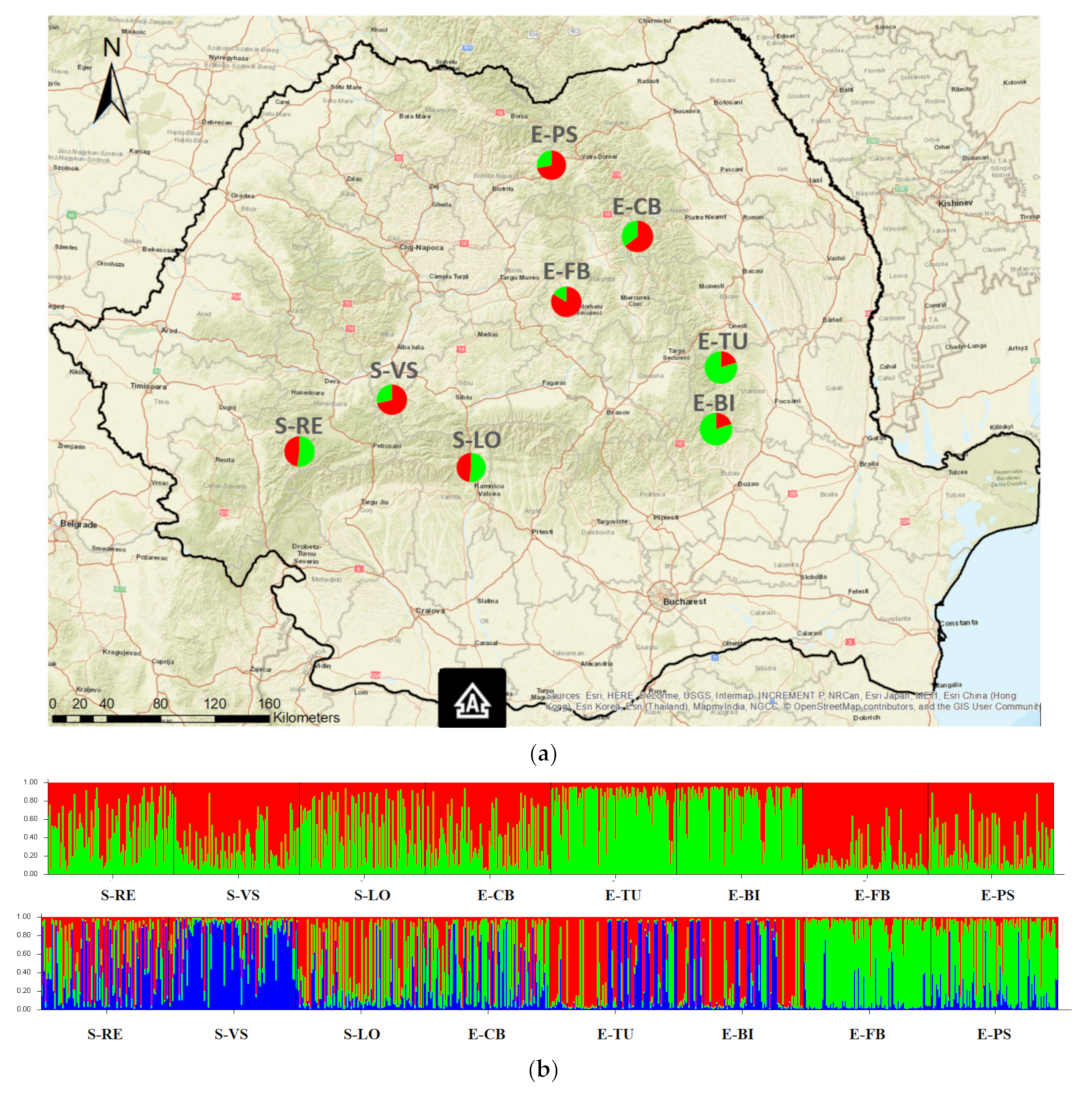
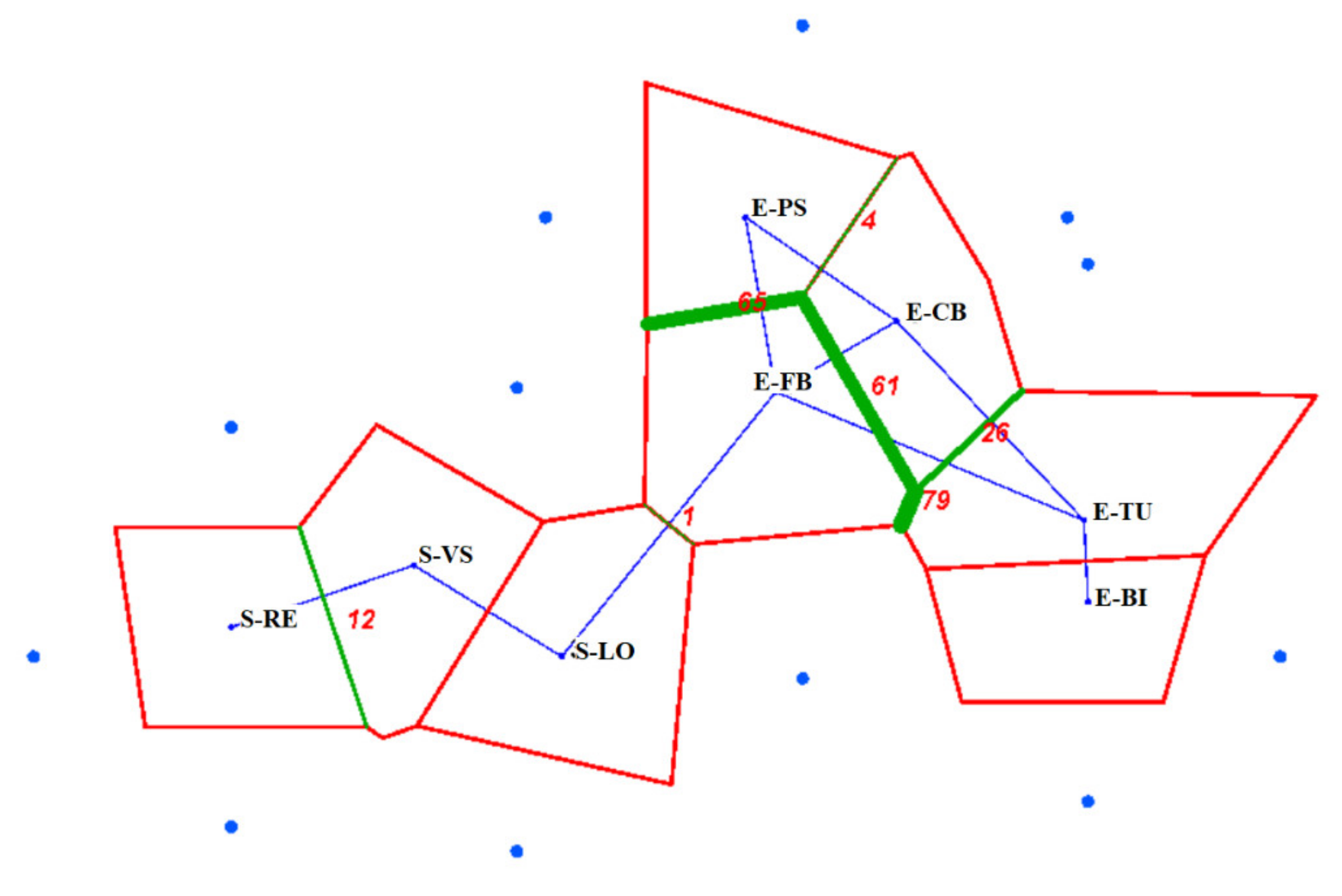
3.2. Population Genetic Structure

A two-cluster structure had the strongest statistical support in our sample (Figure 1b and Figure S1, Supplementary Materials). The highest value of Δk statistics (19.9) was obtained for k = 2 (Figure S1, Supplementary Materials). Two Scots pine populations located on the outward-oriented side of the Southeastern Carpathian arch (E-BI and E-TU) showed the highest membership values in one of the two genetic clusters (in green color in Figure 1). In contrast, the two peat bog populations (E-FB and E-PS) and one Southern Carpathian population located on rocky slopes (S-VS) showed a higher membership in the second genetic cluster (in red color in Figure 1). The other three populations were very admixed. However, when having three genetic clusters (k = 3), the two peat bog Eastern Carpathian populations split from the Southern Carpathian population (Figure 1b).
A genetic barrier prediction analysis detected one barrier against gene flow with strong bootstrap support (61–79%) (Figure 2), which delimited a group of four Eastern Carpathian populations (E-PS, E-CB, E-TU, and E-BI). A second but weak barrier (26% bootstrap support) separated two Eastern Carpathian populations (E-TU and E-BI) located on the outward-oriented side of the Eastern Carpathian arch. A third very weak barrier (12% bootstrap support) was detected between two populations from the Southern Carpathian Mountains (S-RE and S-LO).

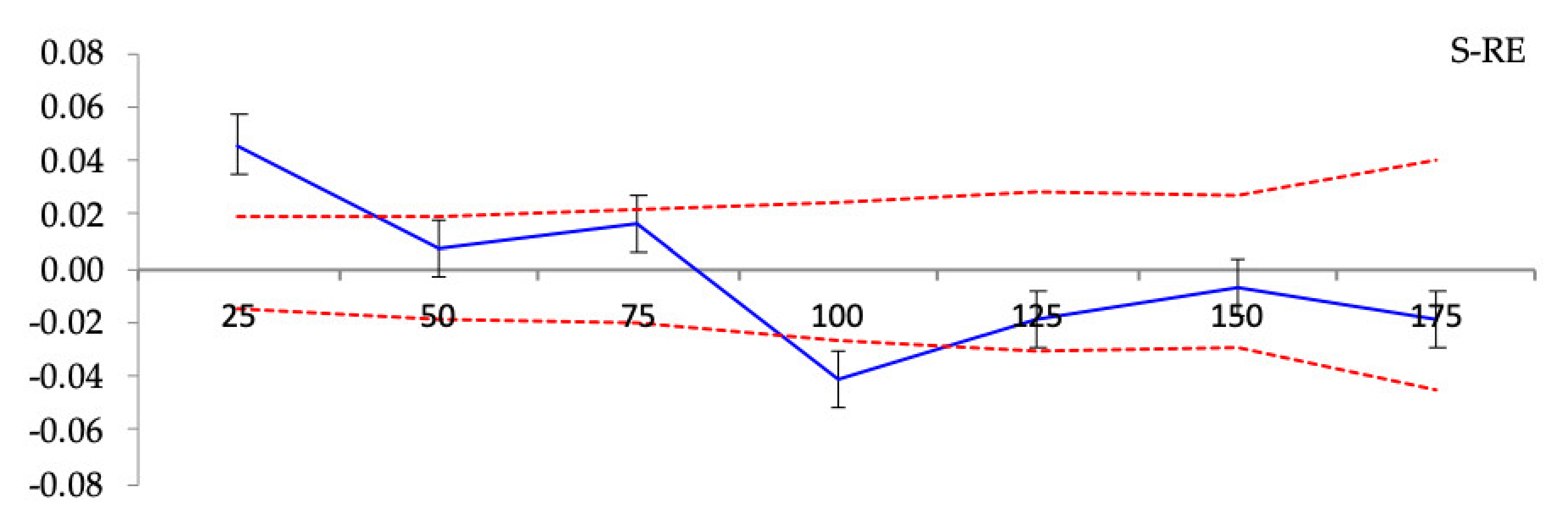
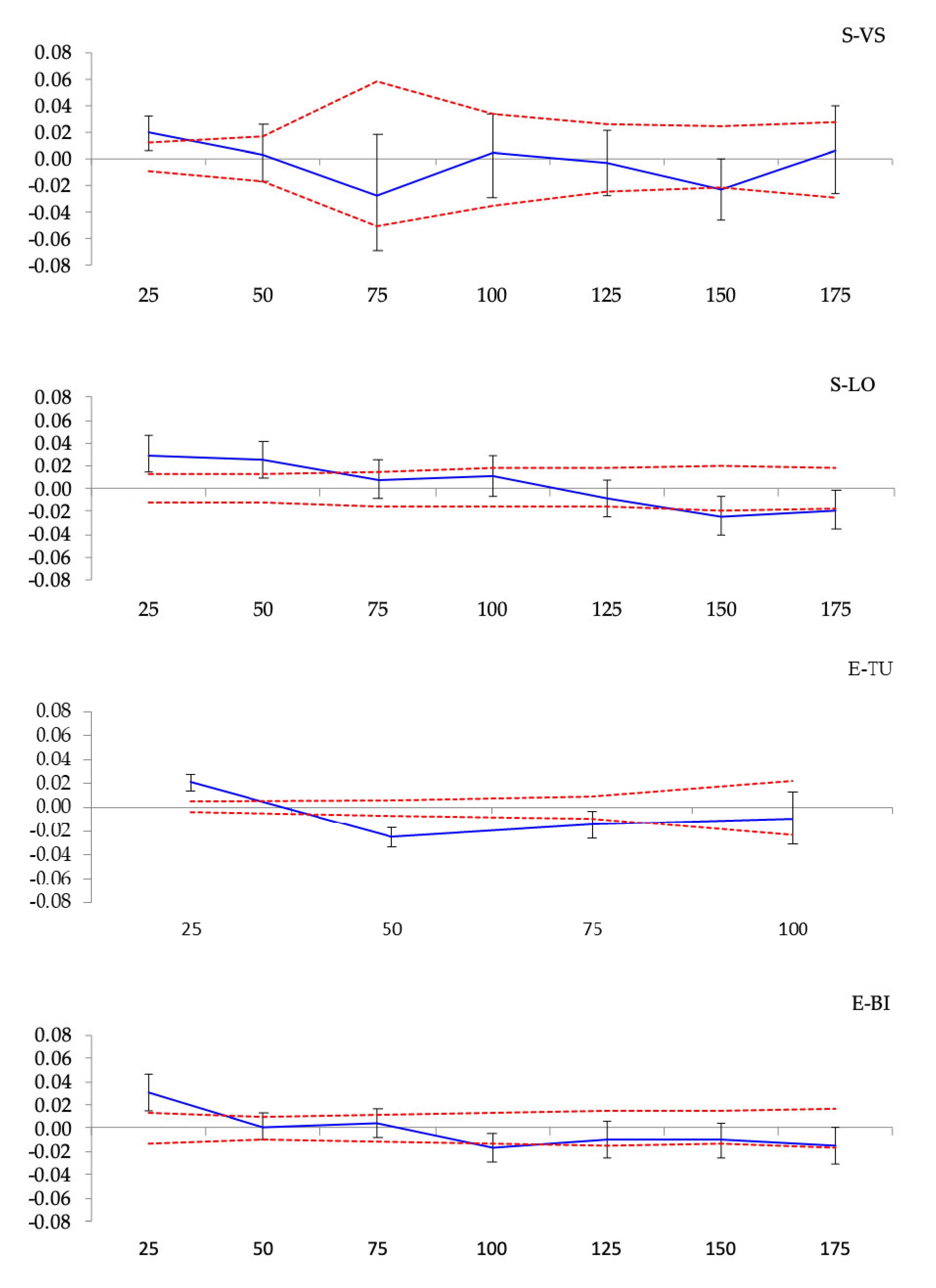
3.3. Spatial Genetic Structure

A nonrandom spatial distribution of genotypes within Scots pine populations was found at six out of the seven locations (Figure 3). Values of the correlation coefficient r were positive and significant in the first distance class (0–25 m) for six populations. In two populations (S-VS and E-FB), the correlation coefficient was significantly positive for the first two distance classes (up to 50 m). The spatial distribution of Scots pine genotypes appeared to be random only in one peat bog population (E-PS).
The value of the Sp statistic varied greatly, ranging from 0.0011 to 0.0201 in populations E-PS and E-TU, respectively, with an average value of 0.0100. The value of bF was significantly different from zero in all populations (Table 4).

4. Discussion

A relatively high level of genetic diversity (He = 0.697) was observed in relict Scots pine populations sampled in Eastern and Southern Carpathian Mountains. A similar value (He = 0.681) was obtained for one Scots pine population in Scandinavia [48], and higher genetic diversity was observed in Central Europe (He = 0.859), as well as in Italy (He = 0.810–0.847) and the Iberian Peninsula (0.810), on the basis of nSSR markers [49,50,51,52]. Slightly lower values were reported for Scots pine in previous studies on Romanian populations including both natural populations and plantations with unknown material [29] or only natural populations from the Eastern Carpathians and Apuseni Mountains, except for one population that was located in the Southern Carpathians [23]. However, these differences have to be treated with caution since different nSSRs were employed in every study. For example, our set of nSSRs had five out of the eight markers used in a previous study on natural Scots pine populations [23] and was almost completely different compared to [29].
Scots pine peat bog populations (E-PB and E-PS) show lower genetic diversity, He = 0.658 and He = 0.635, respectively, compared with populations that grow on nutrient-poor soils or on rocks in the Carpathian Mountains. Interestingly, the same pattern can be observed for populations sampled in the same region in a previous study [23]. A lower genetic diversity of Scots pine in peat bog populations might be explained by extreme environmental conditions, small population size, and human interventions. Scots pine peat bog populations are found on flat terrain and are more accessible compared to natural Scots pine populations located on rocky steep slopes in Eastern and Southern Carpathian Mountains [28]. The mean number of alleles and the number of private alleles also have the lowest values in the peat bog populations. These populations grow in habitats with extreme natural conditions, where a strong selection pressure is assumed, which might potentially lead to a reduction of genetic diversity. No signs of recent bottlenecks were revealed in our analysis but we used only eight nSSR markers. Interestingly, most of the private alleles were observed in the Southern Carpathian populations that grow on rocky slopes. Sampling in such small, relict populations was very difficult because of the rocky terrain. This fact supports the hypothesis that sampled Southern Carpathian populations are untouched by man and may harbor rare variants. In a recent study [53], the only Scots pine population sampled in the Southern Carpathians belongs to a gene pool typical for populations from the Western Carpathians in Hungary and the Apuseni Mountains, and not to a second gene pool corresponding to Eastern Carpathian populations. The region of Eastern Carpathians is considered a distinct glacial refugium for Scots pine [23].
The values of the fixation index (FIS) observed in our study are in agreement with those previously reported in Scots pine [49,51]. Moreover, only in two out of the eight populations, the FIS values were positive and differed significantly from zero, thus indicating an excess of homozygote individuals. Homozygote excess is a common phenomenon in conifer species and may be the result of selection against heterozygotes, assortative mating, or the presence of null alleles [54]. However, isolated and relict Scots pine populations from the Apennine Mountains do not show any significant excess of homozygotes [49], which is also the case in the majority of our Carpathian populations.
A relatively high level of genetic differentiation among Eastern and Southern Carpathian populations was revealed by AMOVA (6%), which is consistent with previous reports on Scots pine peripheral populations from Southeastern Europe [23,49,50]. Past demographic events rather than limited recent gene flow may explain this pattern of among population differentiation at nuclear level [23].
A weak geographic structure, with many admixed populations, was revealed by our analysis. No information about the geographic location of the populations was taken into consideration when running STRUCTURE software, compared to a previous study that used this kind of data (with LocPrior) [23]. The present-day population structure is a consequence of interglacial and postglacial evolutionary history of Scots pine in the Carpathian region. The existence of glacial refugia in the Carpathians [24,25], an admixture of phylogenetic lineages, and population expansions and contractions may have influenced the current gene pool of the species [23,29]. At present, Scots pine is able to survive only in extreme site conditions (e.g., peat bogs, rocks), i.e., ecological niches in which it still remains more competitive than other broadleaved and conifer species [28].
According to STRUCTURE analysis, the two Scots pine populations located in the outward-oriented side of the Eastern Carpathian arch (E-TU and E-BI) are genetically very similar. A genetic discontinuity between this group of two populations and the rest of the Eastern Carpathian populations is supported by BARRIER analysis. Furthermore, the group of the two peat bog populations seems very distinct in STRUCTURE analysis (without LocPrior) but there is apparently a relatively strong genetic discontinuity between the two peat bog populations according to BARRIERS. However, when information on the geographic location was given in STRUCTURE, the peat bog population E-FB appeared to be in a different genetic cluster than the peat bog population E-PS (data not shown); thus, the results of two analyses were eventually congruent. Moreover, the same peat bog population E-FB is located to the inside of the Carpathian arch, being the most central Scots pine population in our sample and, thus, more isolated from the other Eastern Carpathian populations. As suggested by previous results [23], no strong barrier was detected between Eastern and Southern Carpathian populations.

Spatial Genetic Structure

A statistically significant SGS was detected in nearly all studied Scots pine populations. Limited gene dispersal by pollen and seed in accordance with isolation by distance hypothesis may explain the pattern of SGS [9]. Most seeds fell under the canopy of mother trees in relict, mountainous Scots pine populations in Southern Spain [55]. The existence of SGS is expected in untouched, natural populations, even at the adult stage, as was the case in our study. For example, SGS was detected in an old-growth Eastern white pine forest [56] or in a natural, mixed oak forest [12]. The lack of SGS in one peat bog Scots pine population (E-PS) might be explained by the history of the stand, including human interventions, as well as by the sampling design. Thus, sampling of nearby, presumably related individuals up to 15–20 m was, in general, avoided. This fact might have been influenced the strength of SGS in sampled Scots pine populations.
The strength of the SGS, as indicated by the Sp statistics, varied greatly among our Scots pine populations. However, the mean value across populations (0.0100) obtained in our study is consistent with Sp values reported for outcrossing (0.0126) and tree species (0.0102), respectively [9]. The strength of SGS was slightly lower in two mature managed stands of Scots pine (range: 0.0045–0.0098) [15]. A weaker SGS (Sp = 0.0018) was reported for Alpine populations of P. cembra, a species with bird-mediated seed dispersal [13]. The variation in Sp value may be connected with the sampling scheme and population density. Thus, sampling of groups of individuals at different locations hundreds of meters apart within two mountainous Scots pine populations, because not enough individual trees were found at each location, might explain the lower values for the Sp statistic, 0.0036 and 0.0049, in populations S-RE and S-VS, respectively. The Sp value is lower in high-density as compared with low-density populations [9]. This might be an explanation for the lowest Sp value (0.0012) obtained in the relatively high-density population E-PS. The highest Sp value was calculated for population E-TU (0.0207), which had a lower density when compared to other sampled populations. Similar values (0.02–0.026) were reported in small, isolated remnants of maritime pine in the Iberian Peninsula [6]. Deviations from random mating, a lower population density, and potential grouping of reproductive individuals might explain a significant and stronger SGS in small and isolated populations compared to continuous ones [6].
A limitation of our study is the low number of nuclear genetic markers used. However, the number of SSR makers we employed is very similar to recent studies on population genetic structure in Scots pine [23,29]. Furthermore, different sampling schemes (e.g., along one or two transects, consisting of more subpopulations) within Scots pine populations were adopted because of both the spatial configuration of the terrain in the Carpathian Mountains and the scattered distribution of native Scots pine individual trees.

5. Conclusions

The present study, along with previous reports on genetic diversity in Carpathian populations [23], may contribute to the development of a strategy for sustainable management and conservation of the last remnants of Scots pine in the Romanian Carpathians. Scots pine plantations were established with seed imported from other regions (e.g., presumably Central Europe) without a strict record of this transfer [28]. Unfortunately, the use of local seed as reproductive material for forestry purposes was completely neglected. The conservation of Scots pine genetic resources in the Carpathian Mountains should not rely exclusively on in situ conservation units. The establishment of ex situ conservation stands should be an alternative for a better conservation and use of this unique gene pool.
Our study, which was based on the sampling of native populations to both sides of the Carpathian Arch, confirms previous reports that indicate relatively high genetic diversity within populations in spite of a reduction and recent fragmentation of the Scots pine distribution area. We found evidence for lower genetic diversity in peat bog Scots pine populations, compared to populations that grow on nutrient-poor soils and rocky slopes in the Carpathian Mountains. A weak geographic structure of genetic diversity along Southern and Eastern Carpathians was revealed, which may be explained by the postglacial admixture of populations originating from different glacial refugia that existed in the region. The patterns of SGS detected in natural Scots pine populations can be explained by limited seed dispersal, as well as by other factors such as spatial configuration of the population, sampling scheme, and population density.

Supplementary Materials

The following are available online at https://www.mdpi.com/1999-4907/11/10/1047/s1: Figure S1. Estimation of population structure using LnP(D)-derived Δk for determining the optimum number of subpopulations. The maximum value of delta k was found to be at k = 2.

Author Contributions

Conceptualization, N.S., G.M. and A.L.C.; methodology, E.C., N.S. and A.L.C.; software, E.C. and A.L.C.; validation, N.S. and A.L.C.; formal analysis, N.S.; investigation, N.S., E.C. and A.L.C.; resources, G.M. and N.S.; data curation, E.C.; writing—original draft preparation, N.S. and E.C.; writing—review and editing, N.S., G.M., E.C. and A.L.C.; visualization, E.C.; supervision, A.L.C.; project administration, N.S. and G.M.; funding acquisition, N.S. and G.M. All authors have read and agreed to the published version of the manuscript.

Funding

This study was conducted within the GENCLIM project—Evaluation of the adaptive genetic potential of the main coniferous species for a sustainable forest management in the context of climate change, contract no. 151/2014, project financed by UEFISCDI—PN-II-PCCA-2013.

Acknowledgments

We are indebted to numerous colleagues from the forest districts across the country for assisting us during the sampling. We thank the three anonymous reviewers for their suggestions to improve the manuscript.

Conflicts of Interest

All authors have read and agreed to the published version of the manuscript.

References

  1. Habel, J.C.; Assmann, T. Relict Species: Phylogeography and Conservation Biology; Springer: Berlin/Heidelberg, Germany, 2010; ISBN 9783540921608. [Google Scholar]
  2. Hampe, A.; Petit, R.J. Conserving biodiversity under climate change: The rear edge matters. Ecol. Lett. 2005, 8, 461–467. [Google Scholar] [CrossRef] [PubMed] [Green Version]
  3. Fady, B.; Aravanopoulos, F.A.; Alizoti, P.; Mátyás, C.; von Wühlisch, G.; Westergren, M.; Belletti, P.; Cvjetkovic, B.; Ducci, F.; Huber, G.; et al. Evolution-based approach needed for the conservation and silviculture of peripheral forest tree populations. For. Ecol. Manag. 2016, 375, 66–75. [Google Scholar] [CrossRef] [Green Version]
  4. Alberto, F.J.; Aitken, S.N.; Alía, R.; González-Martínez, S.C.; Hänninen, H.; Kremer, A.; Lefèvre, F.; Lenormand, T.; Yeaman, S.; Whetten, R.; et al. Potential for evolutionary responses to climate change—Evidence from tree populations. Glob. Chang. Biol. 2013, 19, 1645–1661. [Google Scholar] [CrossRef] [PubMed] [Green Version]
  5. Eckert, C.G.; Samis, K.E.; Lougheed, S.C. Genetic variation across species’ geographical ranges: The central–marginal hypothesis and beyond. Mol. Ecol. 2008, 17, 1170–1188. [Google Scholar] [CrossRef] [PubMed]
  6. De-Lucas, A.I.; GonzÁlez-MartÍnez, S.C.; Vendramin, G.G.; Hidalgo, E.; Heuertz, M. Spatial genetic structure in continuous and fragmented populations of Pinus pinaster Aiton. Mol. Ecol. 2009, 18, 4564–4576. [Google Scholar] [CrossRef]
  7. Epperson, B.K. Spatial Structure of Genetic Variation within Populations of Forest Trees. In Population Genetics of Forest Trees; Springer: Dordrecht, The Netherlands, 1992; pp. 257–278. [Google Scholar] [CrossRef]
  8. Piotti, A.; Leonardi, S.; Heuertz, M.; Buiteveld, J.; Geburek, T.; Gerber, S.; Kramer, K.; Vettori, C.; Vendramin, G.G. Within-population genetic structure in beech (Fagus sylvatica L.) stands characterized by different disturbance histories: Does forest management simplify population substructure? PLoS ONE 2013, 8, e73391. [Google Scholar] [CrossRef]
  9. Vekemans, X.; Hardy, O.J. New insights from fine-scale spatial genetic structure analyses in plant populations. Mol. Ecol. 2004, 13, 921–935. [Google Scholar] [CrossRef]
  10. Budde, K.B.; González-Martínez, S.C.; Navascués, M.; Burgarella, C.; Mosca, E.; Lorenzo, Z.; Zabal-Aguirre, M.; Vendramin, G.G.; Verdú, M.; Pausas, J.G.; et al. Increased fire frequency promotes stronger spatial genetic structure and natural selection at regional and local scales in Pinus halepensis Mill. Ann. Bot. 2017, 119, 1061–1072. [Google Scholar] [CrossRef] [Green Version]
  11. Morton, N.E. Isolation by Distance. In Brenner’s Encyclopedia of Genetics, 2nd ed.; Elsevier Science: San Diego, CA, USA, 2013; Volume 28, p. 139. ISBN 9780080961569. [Google Scholar]
  12. Valbuena-Carabana, M.; Gonzalez-Martinez, S.C.; Hardy, O.J.; Gil, L. Fine-scale spatial genetic structure in mixed oak stands with different levels of hybridization. Mol. Ecol. 2007, 16, 1207–1219. [Google Scholar] [CrossRef]
  13. Mosca, E.; Di Pierro, E.A.; Budde, K.B.; Neale, D.B.; González-Martínez, S.C. Environmental effects on fine-scale spatial genetic structure in four Alpine keystone forest tree species. Mol. Ecol. 2018, 27, 647–658. [Google Scholar] [CrossRef]
  14. Curtu, A.L.; Craciunesc, I.; Enescu, C.M.; Vidalis, A.; Sofletea, N. Fine-scale spatial genetic structure in a multi-oak-species (Quercus spp.) forest. IForest 2015, 8, 324–332. [Google Scholar] [CrossRef] [Green Version]
  15. González-Díaz, P.; Jump, A.S.; Perry, A.; Wachowiak, W.; Lapshina, E.; Cavers, S. Ecology and management history drive spatial genetic structure in Scots pine. For. Ecol. Manag. 2017, 400, 68–76. [Google Scholar] [CrossRef] [Green Version]
  16. Naydenov, K.; Senneville, S.; Beaulieu, J.; Tremblay, F.; Bousquet, J. Glacial vicariance in Eurasia: Mitochondrial DNA evidence from Scots pine for a complex heritage involving genetically distinct refugia at mid-northern latitudes and in Asia Minor. BMC Evol. Biol. 2007, 7, 233. [Google Scholar] [CrossRef] [PubMed] [Green Version]
  17. Sebastiani, F.; Pinzauti, F.; Kujala, S.T.; González-Martínez, S.C.; Vendramin, G.G. Novel polymorphic nuclear microsatellite markers for Pinus sylvestris L. Conserv. Genet. Resour. 2012, 4, 231–234. [Google Scholar] [CrossRef]
  18. Curt, T.; Prévosto, B. Rooting strategy of naturally regenerated beech in Silver birch and Scots pine woodlands. Plant Soil 2003, 255, 265–279. [Google Scholar] [CrossRef]
  19. Mátyaás, C.; Ackzell, L.; Samuel, C.J.A. EUFORGEN Technical Guidelines for Genetic Conservation and Use for Scots Pine (Pinus sylvestris); International Plant Genetic Resources Institute: Rome, Italy, 2004; 6. [Google Scholar]
  20. Picon-Cochard, C.; Coll, L.; Balandier, P. The role of below-ground competition during early stages of secondary succession: The case of 3-year-old Scots pine (Pinus sylvestris L.) seedlings in an abandoned grassland. Oecologia 2006. [Google Scholar] [CrossRef]
  21. Egnell, G. Effects of slash and stump harvesting after final felling on stand and site productivity in Scots pine and Norway spruce. For. Ecol. Manag. 2016. [Google Scholar] [CrossRef]
  22. Hebda, A.; Wójkiewicz, B.; Wachowiak, W. Genetic characteristics of Scots pine in Poland and reference populations based on nuclear and chloroplast microsatellite markers. Silva Fenn. 2017, 51, 1–17. [Google Scholar] [CrossRef] [Green Version]
  23. Tóth, E.G.; Vendramin, G.G.; Bagnoli, F.; Cseke, K.; Höhn;, M. High genetic diversity and distinct origin of recently fragmented Scots pine (Pinus sylvestris L.) populations along the Carpathians and the Pannonian Basin. Tree Genet. Genomes 2017, 13. [Google Scholar] [CrossRef]
  24. Prus-Głowacki, W.; Urbaniak, L.; Bujas, E.; Curtu, A.L. Genetic variation of isolated and peripheral populations of Pinus sylvestris (L.) from glacial refugia. Flora Morphol. Distrib. Funct. Ecol. Plants 2012. [Google Scholar] [CrossRef]
  25. Tanţǎu, I.; Feurdean, A.; de Beaulieu, J.L.; Reille, M.; Fǎrcaş, S. Holocene vegetation history in the upper forest belt of the Eastern Romanian Carpathians. Palaeogeogr. Palaeoclimatol. Palaeoecol. 2011. [Google Scholar] [CrossRef]
  26. San-Miguel-Ayanz, J.; de Rigo, D.; Caudullo, G.; Houston Durrant, T.; Mauri, A. European Atlas of Forest Tree Species; Publications Office of the European Union: Brussels, Belgium, 2016; ISBN 9789279367403. [Google Scholar]
  27. Feurdean, A.; Tanţâu, I.; Fârcaş, S. Holocene variability in the range distribution and abundance of Pinus, Picea abies, and Quercus in Romania; implications for their current status. Quat. Sci. Rev. 2011. [Google Scholar] [CrossRef]
  28. Şofletea, N.; Curtu, A.L. Dendrologie; Editura Universității Transilvania: Brasov, Romania, 2007; ISBN 9789736358852. [Google Scholar]
  29. Bernhardsson, C.; Floran, V.; Ganea, S.L.; García-gil, M.R. Forest Ecology and Management Present genetic structure is congruent with the common origin of distant Scots pine populations in its Romanian distribution. For. Ecol. Manag. 2016, 361, 131–143. [Google Scholar] [CrossRef]
  30. Feurdean, A.; Wohlfarth, B.; Björkman, L.; Tantau, I.; Bennike, O.; Willis, K.J.; Farcas, S.; Robertsson, A.M. The influence of refugial population on Lateglacial and early Holocene vegetational changes in Romania. Rev. Palaeobot. Palynol. 2007. [Google Scholar] [CrossRef]
  31. Doyle, J.; Doyle, J. A rapid DNA isolation procedure for small quantities of fresh leaf tissue. Phytochem. Bull. 1987, 19, 11–15. [Google Scholar]
  32. Soranzo, N.; Provan, J.; Powell, W. Characterization of microsatellite loci in Pinus sylvestris L. Mol. Ecol. 1998, 7, 1260–1261. [Google Scholar]
  33. Van Oosterhout, C.; Weetman, D.; Hutchinson, W.F. Estimation and adjustment of microsatellite null alleles in nonequilibrium populations. Mol. Ecol. Notes 2006, 6, 255–256. [Google Scholar] [CrossRef]
  34. Peakall, R.; Smouse, P.E. GenAlEx 6.5: Genetic analysis in Excel. Population genetic software for teaching and research—An update. Bioinform. (Oxf. Engl.) 2012, 28, 2537–2539. [Google Scholar] [CrossRef] [Green Version]
  35. Peakall, R.; Smouse, P.E. genalex 6: Genetic analysis in Excel. Population genetic software for teaching and research. Mol. Ecol. Notes 2006, 6, 288–295. [Google Scholar] [CrossRef]
  36. Weiß, C.H. StatSoft, Inc., Tulsa, OK.: STATISTICA, Version 8. Asta Adv. Stat. Anal. 2007, 91, 339–341. [Google Scholar] [CrossRef]
  37. Pritchard, J.K.; Stephens, M.; Donnelly, P. Inference of population structure using multilocus genotype data. Genetics 2000, 155, 945–959. [Google Scholar] [PubMed]
  38. Evanno, G.; Regnaut, S.; Goudet, J. Detecting the number of clusters of individuals using the software STRUCTURE: A simulation study. Mol. Ecol. 2005, 14, 2611–2620. [Google Scholar] [CrossRef] [PubMed] [Green Version]
  39. Earl, D.A.; von Holdt, B.M. STRUCTURE HARVESTER: A website and program for visualizing STRUCTURE output and implementing the Evanno method. Conserv. Genet. Resour. 2011, 4, 359–361. [Google Scholar] [CrossRef]
  40. Excoffier, L.; Lischer, H.E.L. Arlequin suite ver 3.5: A new series of programs to perform population genetics analyses under Linux and Windows. Mol. Ecol. Resour. 2010, 10, 564–567. [Google Scholar] [CrossRef]
  41. Piry, S.; Luikart, G.; Cornuet, J.M. BOTTLENECK: A computer program for detecting recent reductions in the effective population size using allele frequency data. J. Hered. 1999, 90, 502–503. [Google Scholar] [CrossRef]
  42. Manni, F.; Guerard, E.; Heyer, E. Geographic Patterns of (Genetic, Morphologic, Linguistic) Variation: How Barriers Can Be Detected by Using Monmonier’s Algorithm. Hum. Biol. 2007, 76, 173–190. [Google Scholar] [CrossRef]
  43. Monmonier, M.S. Maximum-Difference Barriers: An Alternative Numerical Regionalization Method*. Geogr. Anal. 2010, 5, 245–261. [Google Scholar] [CrossRef]
  44. Dieringer, D.; Schlötterer, C. MICROSATELLITE ANALYSER (MSA): A platform independent analysis tool for large microsatellite data sets. Mol. Ecol. Notes 2003, 3, 167–169. [Google Scholar] [CrossRef]
  45. Smouse, P.E.; Peakall, R. Spatial autocorrelation analysis of individual multiallele and multilocus genetic structure. Heredity 1999, 82, 561–573. [Google Scholar] [CrossRef] [Green Version]
  46. Hardy, O.J.; Vekemans, X. SPAGeDi 1.5 a Program for Spatial Pattern Analysis of Genetic Diversity User’s Manual. Mol. Ecol. Notes 2002, 2, 618–620. Available online: https://www2.ulb.ac.be/sciences/lagev/fichiers/manual_SPAGeDi.pdf (accessed on 7 November 2019). [CrossRef] [Green Version]
  47. Loiselle, B.A.; Sork, V.L.; Nason, J.; Graham, C. Spatial genetic structure of a tropical understory shrub, PSYCHOTRIA OFFICINALIS (RuBIACEAE). Am. J. Bot. 1995, 82, 1420–1425. [Google Scholar] [CrossRef]
  48. Ganea, S.; Ranade, S.S.; Hall, D. Development and transferability of two multiplexes nSSR in Scots pine (Pinus sylvestris L.). J. For. Res. 2015, 26, 361–368. [Google Scholar] [CrossRef]
  49. Scalfi, M.; Piotti, A.; Rossi, M.; Piovani, P. Genetic variability of Italian southern Scots pine (Pinus sylvestris L.) populations: The rear edge of the range. Eur. J. For. Res. 2009. [Google Scholar] [CrossRef]
  50. Belletti, P.; Ferrazzini, D.; Piotti, A.; Monteleone, I.; Ducci, F. Genetic variation and divergence in Scots pine (Pinus sylvestris L.) within its natural range in Italy. Eur. J. For. Res. 2012, 131, 1127–1138. [Google Scholar] [CrossRef] [Green Version]
  51. Nowakowska, J.A.; Zachara, T.; Konecka, A. Genetic variability of Scots pine (Pinus sylvestris L.) and Norway spruce (Picea abies L. Karst.) natural regeneration compared with their maternal stands. For. Res. Pap. 2014, 75, 47–54. [Google Scholar] [CrossRef] [Green Version]
  52. Pavia, I.; Mengl, M.; João Gaspar, M.; Carvalho, A.; Heinze, B.; Lima-Brito, J. Preliminary evidence of two potentialy native populations of Pinus sylvestris L. in Portugal based on nuclear and chloroplast SSR markers. Austrian J. For. Res. 2014, 1, 1–22. [Google Scholar]
  53. Tóth, E.G.; Bede-Fazekas, Á.; Vendramin, G.G.; Bagnoli, F.; Höhn, M. Mid-Pleistocene and Holocene demographic fluctuation of Scots pine (Pinus sylvestris L.) in the Carpathian Mountains and the Pannonian Basin: Signs of historical expansions and contractions. Quat. Int. 2019, 504, 202–213. [Google Scholar] [CrossRef] [Green Version]
  54. Gil MR, G.; Floran, V.; Östlund, L.; Gull, B.A. Genetic diversity and inbreeding in natural and managed populations of Scots pine. Tree Genet. Genomes 2015, 11, 28. [Google Scholar] [CrossRef]
  55. Castro, J.; Gómez, J.M.; García, D.; Zamora, R.; Hódar, J.A. Seed predation and dispersal in relict Scots pine forests in southern Spain. Plant Ecol. 1999, 145, 115–123. [Google Scholar] [CrossRef]
  56. Marquardt, P.E.; Echt, C.S.; Epperson, B.K.; Pubanz, D.M. Genetic structure, diversity, and inbreeding of eastern white pine under different management conditions. Can. J. For. Res. 2007, 37, 2652–2662. [Google Scholar] [CrossRef] [Green Version]
Figure 1. Genetic structure and geographical distribution of eight natural Scots pine populations (a). Geographic location of each sampled populations and their color-coded grouping. The acronyms stand for the population code in Table 1. (b) Estimated population structure for k = 2 (the upper part) and k = 3, assignment.
Forests 11 01047 g001
Figure 2. Identification of predicted genetic barriers among eight Scots pine populations, predicted by BARRIER v.2.2 software (the genetic barriers are shown in green bold lines with bootstrap values) on the basis of Nei’s genetic distance matrix.
Forests 11 01047 g002
Figure 3. Multilocus spatial–genetic correlograms of genetic and geographic distance in seven Scots pine populations. The y-axis is the genetic correlation coefficient (r), and the x-axis is the distance class (m); confidence intervals (95%) were calculated using permutation tests (red lines), and bootstrapped 95% confidence error bars around r are also shown.
Forests 11 01047 g003aForests 11 01047 g003bForests 11 01047 g003c
Table 1. Geographic location of the sampled Scots pine population (S—Southern Carpathian Mountains; E—Eastern Carpathian Mountains; R—rocky slopes; A—acidic and nutrient-poor soils, in areas without rock or skeleton in the upper horizons of the soil; PB—peat bog).
No.PopulationAcronymEcotypeSample SizeGeographic Location
LatitudeLongitudeAltitude (m)
1.RetezatS-RER9645°26′22°46′680–750
45°24′22°46′890–925
2.Valea SebeșuluiS-VSR9645°42′23°36′750–1070
45°42′23°35′730–780
3.LotrișorS-LOR9645°18′24°16′340–510
4.Cheile BicazuluiE-CBR9646°49′25°49′1060–1110
5.TulniciE-TUA9645°55′26°36′580–610
6.BisocaE-BIA9645°33′26°40′930–950
7.Fântâna BrazilorE-FBPB9646°30′25°15′950–960
8.Poiana StampeiE-PSPB9647°18′25°07′920
Table 2. Standard genetic parameters in Scots pine population (Na—number of alleles; Ne—number of effective alleles; He—expected heterozygosity; FIS—inbreeding coefficient; Pa—number of private alleles; SE—standard error).
PopulationEcotype NaNeHeFISPa
S-RERMean9.7504.5530.7240.1623
SE0.9770.6980.0620.104
S-VSRMean10.5005.1650.7330.0494
SE2.0621.1140.0570.090
S-LORMean11.7506.2260.7310.168 *4
SE2.2891.5900.0780.061
E-CBRMean10.7505.2220.6720.1545
SE2.2501.4680.0870.088
E-TUAMean10.3755.2900.7100.1640
SE1.9361.1360.0880.080
E-BIAMean10.2505.2460.7110.1380
SE1.9801.0960.0880.083
E-FBPBMean8.7503.4880.658−0.0462
SE1.9340.4630.0650.073
E-PSPBMean9.3754.2140.6350.187 *0
SE2.2991.0930.0940.066
TotalMean10.1884.9250.6970.12218
SE0.6770.3910.0270.029
* Significant FIS values (p < 0.05) are indicated by an asterisk.
Table 3. Analysis of molecular variance (AMOVA).
SourceDegrees of FreedomSum of SquaresMean SquaresEstimated VariationPercent of Variation
Among population7385.25555.0360.4956%
Within population7605711.8337.5167.51694%
Total7676097.089 8.011100%
Table 4. Parameters describing spatial genetic structure (F1—average of kinship coefficient between individuals of the first distance class (0–25 m); bF (b-log)—slope of the regression of kinship coefficient Fij; Sp—intensity of spatial genetic structure; (±SE)—standard error; (95% CI)—95% confidence intervals; * p < 0.05; ** p < 0.01; *** p < 0.001).
PopulationF1bF (b-log) (±SE)Sp = −bF/(1 − F1)
(95% CI)
S-RE0.0137 *−0.0036 ± 0.0041 ***0.0036
(0.0004–0.0081)
S-VS0.0875 **−0.0046 ± 0.0041 ***0.0049
(0.0021–0.0087)
S-LO0.0187 **−0.0071 ± 0.0047 ***0.0072
(0.0026–0.0168)
S-TU0.0277 *−0.0201 ± 0.0493 **0.0207
(0.0021–0.0239)
S-BI0.0227 *−0.0136 ± 0.0102 **0.0139
(0.0031–0.0356)
S-FB0.0446 **−0.0175 ± 0.0102 **0.0183
(0.0036–0.0303)
S-PS−0.0007−0.0011 ± 0.0052 ***0.0011
(−0.0033–0.0131)

