Abstract
Background and Objectives: Continuous cover forestry is of increasing importance, but operational forest growth models are still lacking. The debate is especially open if more complex spatial approaches would provide a worthwhile increase in accuracy. Our objective was to compare a nonspatial versus a spatial approach for individual Norway spruce tree growth models under single-tree selection cutting. Materials and Methods: We calibrated nonlinear mixed models using data from a long-term experiment in Finland (20 stands with 3538 individual trees for 10,238 growth measurements). We compared the use of nonspatial versus spatial predictors to describe the competitive pressure and its release after cutting. The models were compared in terms of Akaike Information Criteria (AIC), root mean square error (RMSE), and mean absolute bias (MAB), both with the training data and after cross-validation with a leave-one-out method at stand level. Results: Even though the spatial model had a lower AIC than the nonspatial model, RMSE and MAB of the two models were similar. Both models tended to underpredict growth for the highest observed values when the tree-level random effects were not used. After cross-validation, the aggregated predictions at stand level well represented the observations in both models. For most of the predictors, the use of values based on trees’ height rather than trees’ diameter improved the fit. After single-tree selection cutting, trees had a growth boost both in the first and second five-year period after cutting, however, with different predicted intensity in the two models. Conclusions: Under the research framework here considered, the spatial modeling approach was not more accurate than the nonspatial one. Regarding the single-tree selection cutting, an intervention regime spaced no more than 15 years apart seems necessary to sustain the individual tree growth. However, the model’s fixed effect parts were not able to capture the high growth of the few fastest-growing trees, and a proper estimation of site potential is needed for uneven-aged stands.
1. Introduction
Continuous cover forestry (CCF) is a silvicultural system that avoids the use of clear-felling and thus maintains a continuity of woodland conditions across the site [1]. CCF is of increasing interest as a potential solution for delivering a wide range of ecosystem services due to the resulting more complex stand structures [2]. In Fennoscandia, however, [3] highlighted the lack of research data and of adequate growth models for CCF when compared with even-aged plantation forestry, or rotation forestry (RF). In particular, Norway spruce (Picea abies (L.) Karst.) is one of the most economically and ecologically important tree species of Fennoscandia, and also one of the most adapted species that can be managed with CCF principles in the region [3].
Individual tree modeling has long been recognized as the best approach for simulating the growth of irregular stands [4,5]. Since age is not known in CCF stands, functional growth curves [6,7] are often used in RF to model size development as function of time cannot be easily employed. References [8,9] overcame this issue by transforming widely used functional growth curves in age-independent forms. More commonly, tree size increment has been simulated as a function of various tree, stand, and site characteristics with linear or nonlinear models. Novel machine learning techniques have also been used [10].
Tree growth is consistently strongly correlated with the tree size. While bigger trees may have higher growth potential in absolute terms due to more photosynthetic elements, they also have higher respiration costs [11,12] and their relative growth is smaller than that of small trees [13]. Due to this complex relationship between growth and size, many models have employed either linear equations with multiple terms related to tree size [14,15,16,17,18,19] or nonlinear equations [5,20,21,22,23,24,25,26]. In many cases the simulated output of those studies has been a sigmoid-like curve: growth increases with size but eventually reaches a plateau or even decreases.
For stand characteristics, most of the focus has been on describing the negative effect of competition, one of the most important factors affecting tree growth [10]. Different authors have used spatially explicit approaches, that is, where spatial coordinates of the trees are known and specific conditions could be assessed for every individual according to their location, or nonspatial approaches, where competition is calculated regardless of the trees’ locations within the stand. For the spatial approaches, in some cases competition has been calculated considering the interaction between neighboring trees using 2-D representations of the stand [9,23,25,27,28]. In other cases, more complex 3-D representations of the canopy have been used to simulate light interception and availability within the stand [20,29,30,31,32]. In most of the latter 3-D cases, tree growth is a function of light availability and not tree size. Additionally, some models have included a positive effect connected to the structural diversity of the stand, which can provide more space and resource use efficiency [33,34].
The comparison between spatial and nonspatial approaches has not yet reached a conclusive answer. In many cases nonspatial predictors were found as good as spatial ones (e.g., [35,36]). Reference [37] stated that most of such comparisons were carried out in homogenous plantations, while spatial approaches may seem more appropriate in stands with heterogenous structures such as the ones resulting under CCF management. However, the same authors went on demonstrating that nonspatial approaches were sufficiently accurate for most operational growth and yield models also in heterogenous conditions. Additionally, most of either the nonspatial or spatial competition indices considered in the studies reviewed here have been based somehow on the trees’ stem diameters. However, as [38] pointed out, the vertical structure of the forest is equally important, and especially so in heterogenous conditions. Height data is becoming increasingly easier to obtain directly with remote sensing techniques such as aerial laser scanning or digital aerial photography (e.g., [39]) instead of retrieving it indirectly with height–diameter curves, thus in the future it will be more available as input for growth modeling.
The response to cutting has not been often included in modeling growth for CCF. After a release from competition, Norway spruce may take up to around five years, also depending on its age and the intensity of competition prior to release, to acclimatize to the new light conditions (see the extensive review from [40]). Reference [18] did not find significant explicit variables related to thinning, but the study may have been confounded by pooling the data with a rotation forestry dataset [24,26,32,41], including a direct growth boost due to release after cutting, for the latter also due to natural mortality. Reference [23] included an indirect growth boost by simulating a longer crown size for trees left after thinning, which in turn will grant higher growth. A better knowledge of the response after partial cutting in CCF is crucial to compare different intervention scenarios.
Climate and site characteristics have been included in various ways, for example, with very detailed climatic variables, such as mean temperature, mean precipitation, and global radiation [15,17,20,24]; detailed edaphic characteristics, such as nutrients supply, soil type, and depth [14,20,22,24,30]; and detailed topographic variables, such as elevation, slope, and aspect [14,15,22,24,26,42]. Site index, a commonly used parameter in RF representing the dominant height of a stand at a certain age, has sometimes been used also in CCF [15,21,23]. However, the concept is problematic in uneven-aged stands where the age–height relationship is not nearly as straightforward, and it has been sometimes adapted to the uneven-aged structure in different ways [26,43] or substituted with general fertility classes [42]. In Finland, temperature sum (the sum of daily average temperatures in excess of a threshold of 5 °C during the annual growing season) and forest site types have often been used [5,16,18]. In one study [10], it was assessed that the climate variables contributed to around 18% of the variance in tree growth, and site variables to 4%.
The overall objective of this study was to compare the performances of spatial versus nonspatial approaches for Norway spruce individual tree growth modeling in single-tree selection cutting conditions, using nonlinear mixed models. Specifically, using data from fully mapped stands, we wanted to answer the following research questions: (1) Are spatial competition indices and cutting variables more accurate as growth predictors than their nonspatial counterparts? (2) Are variables related to the trees’ height more accurate as growth predictors than their counterparts related to the trees’ diameter? (3) What is the temporal tree-level growth response after single-tree selection cuttings of different intensity?
2. Methods
2.1. Study Material
We used data from a long-term experiment of CCF permanent sample plots involving single-tree selection in 20 Norway spruce-dominated stands in Southern Finland (60°30′–62°30′ N, 25–27 ° E) (Table 1). Most of the stands (16) belonged to the submesic Myrtillus type site classification, or grove-like heath and fresh heath, while the rest (4) to the mesic Oxalis-Myrtillus [44,45]. The stands had been managed with single-tree selection for 25–30 years, and their prior development was also characterized by complex stand structures and partial harvests of variable intensity. The stands had emerged from natural regeneration with irregular initial development, and structural complexity was characteristic for the stands throughout their growth. Utilizing the existing structural complexity, single-tree selection was started in the 1980s. A selection cutting was carried out in all the stands in 1985–1988. After the establishment of the experimental stands in their current form (1991–1996), the selection cutting was repeated in 1996 in 16 stands. Four stands were not harvested in 1996 due to their low growing stock. All stands were harvested again in 2011. All trees with defects or damage were removed first, and then healthy trees mainly from the larger diameter classes (>25 cm) were removed until a target basal area was achieved. All stands can be characterized as truly multiaged (with trees up to 170 years old) and full-storied (in the sense of [46]).

Table 1.
Summary of study sites and tree-level measurements. The methods for calculating some of the variables are described later in the data processing section. Local neighborhoods are circular plots located around each subject tree.
The 20 stands were grouped in five areas, each with 2–7 stands. The stand area was 1.5–2 ha. Within each stand, a single plot 40 m × 40 m was set up in the central part of the stand with good representation of site and structural variation within the stand. The stands were managed similarly within the plot and outside of it. Near the plot borders, the whole neighborhood was considered during the tree selection for cutting. Tree measurements on the plots started in 1991 and were repeated every five growing seasons (only in one case, a plot was measured after six growing seasons and growth values were rescaled accordingly). Species, diameter at breast height (above bark, measured at 1.3 m from the ground in two perpendicular directions with a caliper and then averaged), tree height (measured with a Haglöf Vertex hypsometer, Haglöf Sweden AB, Långsele, Västernorrland, Sverige), height of the crown base, and local coordinates were assessed for each tree during any measurement, carried out before the cutting. See [47,48] for more detailed information on the experimental setting, measurements, and stand properties.
2.2. Data Processing
Since we wanted to precisely assess the effect of thinning, we used only the data since the first detailed recorded thinning (in 1996 or 2011) for each plot (for a total of 64 combinations of plots and growth periods). For each tree we calculated basal area (ba, cm2) as the cross-sectional stem area at 1.3 m from the ground. Our dependent variable was then individual basal area growth (Δba, cm2 year−5), calculated for each alive Norway spruce tree as the difference between two consecutive measurements. Our explanatory variables could be categorized into tree, competition, stand, cutting, and site characteristics. To calculate all spatial variables, as edge correction for trees at the border of the mapped plots, we applied a translation approach [49]. We virtually recreated the stand in a 3 × 3 grid with the original mapped plot as central cell, and in all the other cells, we copied the same plot with the same orientation.
For the tree characteristics, we considered size, as either stem diameter (d, cm) or height (h, m), and live crown ratio (lcr), the ratio between the tree height (h) and the length of the live crown. Due to the nonlinear relationship between growth and size, we tested for d and h various transformations (root, power, and logarithmic) and the use of multiple terms.
For the competition, we calculated various indices, both symmetric (i.e., independent of the relative size of the competing trees) and asymmetric (i.e., where relatively bigger trees would apply higher competition against relatively smaller trees). We considered: basal area sum of all trees (batot, m2 ha−1); height sum of all trees (htot, km ha−1); basal area sum of trees larger than the subject tree (bal, m2 ha−1); height sum of trees taller than the subject tree (htal, km ha−1). We calculated them both with a nonspatial and a spatial approach. For the former, we considered all the alive trees in the plot. For the latter, we considered only the trees within local neighborhoods around each tree, using different radii (namely 5.64 m, 7.97 m, and 9.77 m to reach 100 m2, 200 m2, and 300 m2, respectively). We also estimated the Hegyi’s competition index, calculated both for dbh (diameter at breast height, 1.3 m) and height (hegyiD and hegyiH) according to Equation (1), using all the trees present in the three different local neighborhoods [50]:
where n is the number of trees present in the local neighborhood, sizei and sizej are either the dbh or height, respectively, of the competitor i and of the subject tree j, distanceij is the distance in meters between the two trees. We did not consider a nonspatial equivalent for this index. Such indices calculated for a defined neighborhood could be referred to as semi-spatial indices. Lastly we calculated two spatial indices corresponding to the area potentially available for resources, calculated by means of Voronoi polygons around each subject tree, either with standard polygons (apa, m2) or weighted by means of each tree’s dbh (apaw.d, m2) and height (apaw.h, m2) [37,51] (see Figure 1 for examples and further explanations). Standard polygons were built with the package dismo [52] of R Statistical Software (R Foundation for Statistical Computing: Vienna, Austria) [53], while the code used under R to build the weighted polygons is shown in Supplementary Materials Section S1. We tried both a linear and a square root weight for the size, and a squared distance. The area potentially available is not strictly a competition index as it is expected to be positively correlated with growth, but it expresses the same concept in a different way. Please refer to Table 2 for a summary of all competition indices.
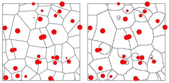
Figure 1.
Examples of standard (left) and weighted (right) Voronoi polygons created starting from the same trees (red points, size proportional to their height). The standard polygon for a tree includes all the area that is closer to that tree. The weighted polygon pushes its boundaries towards neighbors with lower size.
Table 2.
Competition and growing space indices tested. Local neighborhoods include plots of 100, 200, and 300 m2.
For the stand category, we calculated one index of species diversity as the ratio between the total basal area of all spruce trees and the total basal area of all trees (mixba, %). For the nonspatial approach, we considered all the trees in the stand, while for the spatial approach, only the trees in local neighborhoods. We considered two indices of the structural diversity of the dbh and the height distribution: the Gini coefficient (ginid and ginih) [54], calculated with the package ineq [55] of R Statistical Software; and the standard deviation (sdd and sdh). As above, we considered either all trees in the stand or only local neighborhoods. We also considered the plot basal area weighted mean diameter (Dg) and basal area weighted mean height (Hg), as an indication of stand development.
For the cutting characteristics, under the nonspatial approach, we considered the basal area removed during the last intervention relative to the total stand basal area prior to the cutting (bacutp); and similarly, the sum of the trees’ height removed relative to the total (hcutp). Under the spatial approach, we calculated the same for the local neighborhoods. We considered the time after the last cutting using dummy variables as follows: time after cutting class 1 (tac1) if the growing period started immediately after the intervention, tac2 if 6 years after (second measurement period after intervention), and tac3 if 11 years (third measurement period, the maximum in this dataset).
For the site characteristics, we simply considered the forest type using a dummy variable omt, with value of 1 for the stands in the Oxalys-Myrtillus site type and 0 for the other sites, and a climatic continuous variable, tsum, the temperature sum in degree-days [56]. As an alternative to forest type, to describe the site potential, we calculated the mean annual growth of each stand in terms of basal area, averaged throughout all the measurements (mag, m2 ha−1 year−1).
After being used to calculate all predictors, trees with external signs of strong damage as specifically recorded in the field forms were removed from the following growth modeling activities, together with trees showing the largest and the smallest 0.1% of ∆ba values considered as outliers [24].
2.3. Statistical Analyses
We used the following nonlinear mixed model form (Equation (2)), fitted with the package nlme [57] of R Statistical Software, to model the growth of Norway spruce trees:
where Δba was the individual tree growth; a fixed intercept; the explanatory variables; coefficients to be determined during model fitting; , and random nested effects respectively for each area and plot to account for the spatial correlation of trees in the same areas and plots, and for each tree to account for the longitudinal experimental design structure (i.e., the repeated measurements on the same trees); and the error for each measurement. We used a variance function to reduce heteroscedasticity [17,34,58], and an autoregressive structure where correlation is higher for nearby measurement periods than for farther-apart periods [34,59]. With the package nlme, we used the option VarPower for the former (with the formula based on tree basal area) and corrAR1 for the latter.
We prepared two base model structures with all potential explanatory variables: one using only the nonspatial variables, and one only the spatial variables. In both cases, to avoid overfitting, only one symmetric and one asymmetric competition were included (see Table 2). In the spatial model, we compared the same variables calculated with different local neighborhood size. We then reached a final model structure in both cases by removing variables according to the following criteria: lower AIC, better residual distribution, and sound biological validity. We compared the two final models by visual assessment of predictions and residuals, and by means of mean annual bias (MAB) and root mean square error (RMSE). We did so after both autovalidation and a cross-validation with a leave-one-out approach at the plot level [60]. For the latter, we refitted the models 20 times, removing all trees from one plot and then validating the model on the removed data. In this case, we also analyzed the results aggregated at stand level for each measurement period.
3. Results
The diameter distribution in all stands followed a classic reverse J curve: on average more than half of the trees belonging to the smaller classes 5 and 10 cm DBH. However, on average more than half of the stem growth at stand level was realized by the trees in the middle classes from 15 to 25 cm DBH. Figure 2 shows the relative contribution for each diameter class both in terms of number of trees and basal area growth to the stand totals.
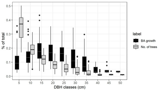
Figure 2.
Contribution to total growth and total number of trees for each diameter class, calculated in every plot and measurement period and shown as boxplots.
The best nonspatial and spatial model structures were very similar, differing only in the kind of asymmetric competition and structural diversity variable used. The models were defined with Equation (3) for the nonspatial and Equation (4) for the spatial:
where h was the tree height (m); lcr the live crown ratio; htot the sum of the height of all trees (km ha−1) as symmetric competition; in the nonspatial model, htal was the sum of the heights of the trees taller than the subject tree (km ha−1), and in the spatial model, hegyih was the Hegyi competition index for height, both as asymmetric competition; bacutp was the basal area removed during cutting relative to the total basal area prior to the intervention; tac1, tac2, and tac3 were dummy variables indicating each progressive five-year period after cutting; mag was the mean annual growth of the stand (m2 ha−1 year−1); in the nonspatial model, sdh was the standard deviation of all tree heights, and in the spatial model, ginih was the Gini coefficient for all tree heights, both as indicator of structural diversity. In the spatial model, htot was calculated for the 300 m2 local neighborhoods of each tree, bacutp and hegyih for the 200 m2 local neighborhoods, and ginih for the 100 m2 local neighborhoods. In all cases except for the cutting intensity, variables based on tree height significantly improved the fit compared to their counterparts based on tree diameter. A nonspatial model with only diameter-related predictors had AIC 68,714, and a spatial one AIC 68,384, both higher than their selected counterparts based mostly on height-related predictors (Table 3), although with comparable RMSE and MAE (please refer to Supplementary Materials Section S2 for more information). The area-level random effect was removed since it did not significantly decrease the AIC.
Table 3.
Summary of the selected nonspatial and spatial models. All parameters were significant with p values < 0.001. AIC is Akaike Information Criteria, RMSE is root mean square error, MAB is mean absolute error. Validation results are provided for both auto-validation with all data and leave-one-out cross-validation at plot level.
Both models fit reasonably well to the observed data. The differences in RMSE and MAB after autovalidation on the training data were negligible between the models (Table 3). Figure 3 shows the fitted values against the observed values (graphs a and b), and the residuals against the fitted values (graphs c and d) for both models.
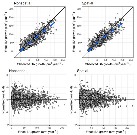
Figure 3.
Results for both models of individual tree growth. (Top row): fitted versus observed values, respectively, for nonspatial and spatial model (dashed blue line: locally estimated scatterplot smoothing curve, or LOESS, fitted to the scatter plot). (Bottom row): normalized residuals versus fitted values, respectively, for nonspatial and spatial model. The continuous black line in all graphs is the identity line.
The size-growth relationship was quasi-sigmoid in both models since they included individual size (in terms of height) as multiple terms. In Figure 4 we predicted growth only as a function of tree height (set to vary throughout the observed range), while we kept the rest of the predictors at the average observed for each five-year period after cutting (accounting for the increase of symmetric competition over time after a thinning). The only exceptions were the asymmetric competition indices (htal and hegyih): a model was constructed for them as a function of tree height (see Supplementary Materials Section S3) and their values were fixed to the model predictions (accounting for the decrease of competition with higher tree size). All random effects were omitted. On average, the predictions were similar to the observed mean in both models, although there was an underestimation for the tallest trees above 20–25 m, especially in the period 11–15 years after cutting. When observing the fitted values of both models with the random effects, there was no such underestimation and the trend closely resembled the locally estimated scatterplot smoothing curve (LOESS) in Figure 4 (results not shown).
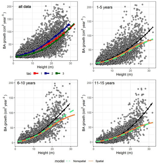
Figure 4.
Individual basal area growth as function of tree height. The points are observed data (with continuous dotted lines as locally estimated scatterplot smoothing curves, or LOESS, estimated directly from the data, not from the models). Top left plot shows all data, and different observed LOESS curves for different time after harvesting classes (tac1): 1–5 years, (tac2): 6–10 years, (tac3): 11–15 years. In the remaining graphs, only specific time after harvesting classes are displayed. The colored dashed and continuous lines are predicted values for the nonspatial and spatial model, respectively, while the black continuous dotted lines the corresponding LOESS curves of the top left graph.
After cross-validation, again there were only negligible differences amongst the two models, both at tree and stand level. In Figure 5, the simulations are compared with the observations, both at tree level and stand level. There was, however, a serious underestimation of growth for the faster growing trees (roughly above basal area growth 150 cm2 year−5, which accounts for only 1% of the total trees in the dataset, and 5% of the total observed growth). Overall, the stand-level results seemed to fit well the observations. Mean annual growth as predictor of site potential, when compared to the forest type OMT/MT dummy variable, strongly decreased the errors in the cross-validation process for both models: with the latter variable, there was a strong negative bias in all MT plots in both models (results not shown).
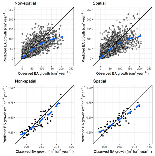
Figure 5.
Cross-validation results for both models of individual tree growth (left column) nonspatial, (right column) spatial; (top row) fitted versus observed individual tree growth; (bottom row) fitted versus observed growth, both aggregated at stand level for each measurement period. The black line in all graphs shows the identity line, the dashed blue line a locally estimated scatterplot smoothing curve for the scatterplot.
Due to the above results, we investigated further the random effects. The tree-level random effects were found to be significantly and slightly positively correlated to the individual tree mean growth (averaged over all the measurement periods), with a Pearson correlation coefficient of 0.35 and 0.33 for the nonspatial and spatial model, respectively. No other significant correlations were found between the model predictors and the tree-level random effects.
For both models, there was a growth boost in both the first and second five-year period after cutting. In Figure 6, this effect is observed for a sample tree of mean height (9 m). Predictions for both models were calculated considering all parameters set at the average observed for each time after cutting period, and only the removed basal area was allowed to vary throughout the observed range. The two models differed in the intensity of the growth boost: it was much higher in the first five-year period for the nonspatial model compared to the second one, while it was of similar intensity in the two five–year periods after cutting for the spatial model. However, the two models agreed that more than 10 years after cutting, the growth could decrease to half the level of the first 10-year period.
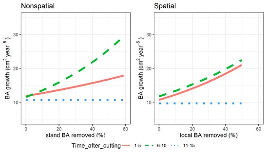
Figure 6.
Individual tree growth response to single-tree selection cutting intensity, measured as percentage of basal area (BA) removed relative to levels prior the cutting, for different times after cutting and models. In the nonspatial model, cutting intensity is calculated at stand level, in the spatial model for the local 200 m2 neighborhood around the subject tree. The lines show the growth of a tree of average height (9 m), when growing either 1–5 years after cutting (continuous line), 6–10 years after (dashed line), or 11–15 years (dotted line).
4. Discussion
Are spatial competition indices and cutting variables more accurate as growth predictors than their nonspatial counterparts? The spatial model, although having a lower AIC than the nonspatial one, did not provide an increase in the model accuracy when looking at the prediction errors, both during the auto- and cross-validation processes. This was in line with previous research [35,36,37]. However, for a full forest growth simulation, the modeling of processes such as regeneration could still require spatial information, since they may be more sensible to local variation in stand density (e.g., [61]). For the spatial model, different predictors had a different local area of effect. For the symmetric competition, the largest area considered (300 m2) provided better results, while for other predictors related to asymmetric competition and the irregular structure, smaller areas provided better results (200 and 100 m2 for the Hegyi and Gini index, respectively). Our spatial approach had a limitation in considering a defined threshold distance for the effect of most of the predictors, apart from the Voronoi polygons that were eventually not included in the final models due to their lower predictive power (i.e., higher AIC). See [62] for a discussion on the matter.
Are variables related to the trees’ height more accurate as growth predictors than their counterparts related to the trees’ diameter? Variables related to height were generally better predictors than their counterparts based on the diameter. Diameter and height are strongly correlated, so it may be expected that they would provide similar results. Nonetheless, it seems that height-related variables better described the competition dynamics for light in the irregular stands considered in this study. It would be interesting to test the same in even-aged forests where there is generally less variation in the vertical structure. The success in fitting a model with only height-related variables has important considerations for future development. Advances in remote sensing with drones and UAV could soon switch the routine tree-level measurement from diameter-based to height-based. Many applications proved it was possible to retrieve the tree diameter from remotely sensed data, and then use such values as inputs for growth simulations [63,64]. However, since tree height may be a comparable or better input at least in vertically diverse forests, there would not be the need of such intermediate steps.
What is the temporal tree-level growth response after single-tree selection cuttings of different intensity? The growth boost in the first 10 years after cutting (for both models) is in line with previous research on release of spruce trees. However, there were contrasting results between models on the intensity of such a boost in the two five-year periods after intervention. [40] concluded that Norway spruce may need up to five years to adapt to the new light environment, depending on size and previous history of the trees. The stands in this study were already being managed with selective cutting for many years before the measurements started, so it may be that the dominated trees were not heavily suppressed and quick to exploit the higher light availability. The growth measurement period of five years may be too coarse to properly identify the finer scale annual response. As a comparison, [41] analyzed yearly growth measurements in irregular coniferous forests in the USA after thinning. Their findings show that the response of coniferous species after release, averaged over five years, was similar in the first two five-year periods after thinning. However, there was a less sharp decline in the third period. For white pine (Pinus strobus L.), [65] found the growth response after release cutting evident already after three years, reaching a maximum around 13 years and then decreasing. According to volume increment compared with control trees, the response was higher in more dominated trees, similar to our findings. In any case, for Finnish conditions, a selection cutting system not more than 15 years apart is supported by the data to sustain a good individual growth. Further study on lighter intensity but more frequent interventions (i.e., every 10 years) could be also investigated, due to the observed lower growth in the period 11–15 years after cutting. We acknowledge that for that period, both models strongly underestimated the growth for the larger trees, indicating a need to improve the fit.
Generally, both models had a sound biological validity. Growth was strongly and nonlinearly correlated with tree size, reaching a peak for the bigger trees only when random effects were not used [5]. However, the random effects simulations suggested a continuous increase with size [66]. Longer live crown ratios were significantly and positively correlated with growth, likely as another indicator of past competition [23]. Both a symmetric and an asymmetric competition index seemed to be necessary to fully describe the tree-level interactions [41]. The irregular vertical structure in the forest (through the standard deviation or Gini coefficient for tree heights) provided a small but significant additional boost to growth, maybe due to better resource use efficiency [33]. An indicator of site productivity estimated from the overall observed growth was necessary as an alternative to climatic variables and the forest site dummy indicators. We are aware that such a predictor cannot be estimated a priori for stands without growth observations, thus other variables should be investigated. Temperature sum did not have significant results, probably due to the limited variability of climatic conditions across the sites.
We observed a correlation between tree random effects and mean tree growth, and underestimation of growth for the faster-growing trees during the cross-validation process. It may be that the fixed effects part of the model was not able to describe the specific causes, such as microfertility variations or genetic profiles, for few faster-growing trees (around 1% of the total, contributing to 5% of the total growth, considering an arbitrary threshold of basal area growth 150 cm2 year−5). This could provide concerns for the applicability of these models outside the calibration data. On the other hand, the cross-validation results aggregated at stand level were promising for both models, suggesting the underestimation of those trees did not affect much the overall growth.
5. Conclusions
We did not find any evidence that a spatial approach is better than a nonspatial one for modeling individual tree growth for Norway spruce stands managed with single-tree selection, when using the nonlinear mixed modeling approach. Variables related to the tree height were in almost all cases better predictors of tree growth than their counterparts based on tree diameter. Selection cutting provided a growth boost proportional to its intensity on remaining trees that were released from competition. The effect lasted for the first 10-year period after cutting, and then disappeared. Even if there were some issues in the models (underestimation of fast-growing trees, need to identify a better site potential variable), the cross-validation results for the nonspatial model provided promising results.
Supplementary Materials
The following are available online at https://www.mdpi.com/1999-4907/11/12/1338/s1, Section S1. Script to calculate weighted Voronoi polygons in R; Section S2. Alternative model structures for trees’ diameter; Section S3. Modeling asymmetric competition as function of tree height.
Author Contributions
Conceptualization, S.B. and M.M.; methodology, S.B.; writing—original draft preparation, S.B.; writing—review and editing, S.B., M.M., J.S., H.S., J.H., S.V.; visualization, S.B. All authors have read and agreed to the published version of the manuscript.
Funding
The study was funded by the MERIKA project from the Natural Resources Institute Finland (LUKE). We declare no conflicts of interest. MM was financially supported by the Academy of Finland (Project numbers 295100 and 327211).
Conflicts of Interest
The authors declare no conflict of interest.
References
- Mason, W. Implementing continuous cover forestry in planted forests: Experience with Sitka Spruce (Picea Sitchensis) in the British Isles. Forests 2015, 6, 879–902. [Google Scholar] [CrossRef]
- Mizunaga, H.; Nagaike, T.; Yoshida, T.; Valkonen, S. Feasibility of silviculture for complex stand structures: Designing stand structures for sustainability and multiple objectives. J. For. Res. 2010, 15, 1–2. [Google Scholar] [CrossRef]
- Kuuluvainen, T.; Tahvonen, O.; Aakala, T. Even-aged and uneven-aged forest management in Boreal Fennoscandia: A review. AMBIO 2012, 41, 720–737. [Google Scholar] [CrossRef] [PubMed]
- Curtis, R.O. Yield tables past and present. J. For. 1972, 70, 28–32. [Google Scholar]
- Pukkala, T.; Lähde, E.; Laiho, O. Species interactions in the dynamics of even- and uneven-aged Boreal Forests. J. Sustain. For. 2013, 32, 371–403. [Google Scholar] [CrossRef]
- Fekedulegn, D.; Mac Siurtain, M.; Colbert, J. Parameter estimation of nonlinear growth models in forestry. Silva Fenn. 1999, 33. [Google Scholar] [CrossRef]
- Paine, C.E.T.; Marthews, T.R.; Vogt, D.R.; Purves, D.; Rees, M.; Hector, A.; Turnbull, L.A. How to fit nonlinear plant growth models and calculate growth rates: An update for ecologists: Nonlinear plant growth models. Methods Ecol. Evolut. 2012, 3, 245–256. [Google Scholar] [CrossRef]
- Tomé, J.; Tomé, M.; Barreiro, S.; Paulo, J.A. Age-independent difference equations for modelling tree and stand growth. Can. J. For. Res. 2006, 36, 1621–1630. [Google Scholar] [CrossRef]
- Quiñonez-Barraza, G.; Zhao, D.; De Los Santos Posadas, H.M.; Corral-Rivas, J.J. Considering neighborhood effects improves individual dbh growth models for natural mixed-species forests in Mexico. Ann. For. Sci. 2018, 75, 78. [Google Scholar] [CrossRef]
- Ou, Q.; Lei, X.; Shen, C. Individual tree diameter growth models of larch–spruce–fir mixed forests based on machine learning algorithms. Forests 2019, 10, 187. [Google Scholar] [CrossRef]
- Givnish, T. Adaptation to sun and shade: A whole-plant perspective. Funct. Plant. Biol. 1988, 15, 63. [Google Scholar] [CrossRef]
- King, D.A. The adaptive significance of tree height. Am. Nat. 1990, 135, 809–828. [Google Scholar] [CrossRef]
- Assmann, E. The Principles of Forest Yield Study; Pergamon: Oxford, UK, 1970. [Google Scholar]
- Sterba, H.; Blab, A.; Katzensteiner, K. Adapting an individual tree growth model for Norway spruce (Picea abies L. Karst.) in pure and mixed species stands. For. Ecol. Manag. 2002, 159, 101–110. [Google Scholar] [CrossRef]
- Andreassen, K.; Tomter, S.M. Basal area growth models for individual trees of Norway spruce, Scots pine, birch and other broadleaves in Norway. For. Ecol. Manag. 2003, 180, 11–24. [Google Scholar] [CrossRef]
- Pukkala, T.; Lähde, E.; Laiho, O. Growth and yield models for uneven-sized forest stands in Finland. For. Ecol. Manag. 2009, 258, 207–216. [Google Scholar] [CrossRef]
- Dănescu, A.; Albrecht, A.T.; Bauhus, J.; Kohnle, U. Geocentric alternatives to site index for modeling tree increment in uneven-aged mixed stands. For. Ecol. Manag. 2017, 392, 1–12. [Google Scholar] [CrossRef]
- Bianchi, S.; Huuskonen, S.; Siipilehto, J.; Hynynen, J. Differences in tree growth of Norway spruce under rotation forestry and continuous cover forestry. For. Ecol. Manag. 2020, 458, 117689. [Google Scholar] [CrossRef]
- Oboite, F.O.; Comeau, P.G. The interactive effect of competition and climate on growth of boreal tree species in western Canada and Alaska. Can. J. For. Res. 2020, 457–464. [Google Scholar] [CrossRef]
- Pretzsch, H.; Biber, P.; Ďurský, J. The single tree-based stand simulator SILVA: Construction, application and evaluation. For. Ecol. Manag. 2002, 162, 3–21. [Google Scholar] [CrossRef]
- Lacerte, V.; Larocque, G.R.; Woods, M.; Parton, W.J.; Penner, M. Calibration of the forest vegetation simulator (FVS) model for the main forest species of Ontario, Canada. Ecol. Modell. 2006, 199, 336–349. [Google Scholar] [CrossRef]
- de-Miguel, S.; Pukkala, T.; Assaf, N.; Bonet, J.A. Even-aged or uneven-aged modelling approach? A case for Pinus brutia. Ann. For. Sci. 2012, 69, 455–465. [Google Scholar] [CrossRef]
- Thurnher, C.; Klopf, M.; Hasenauer, H. MOSES–A tree growth simulator for modelling stand response in Central Europe. Ecol. Modell. 2017, 352, 58–76. [Google Scholar] [CrossRef]
- Rohner, B.; Waldner, P.; Lischke, H.; Ferretti, M.; Thürig, E. Predicting individual-tree growth of central European tree species as a function of site, stand, management, nutrient, and climate effects. Eur. J. For. Res. 2018, 137, 29–44. [Google Scholar] [CrossRef]
- Häbel, H.; Myllymäki, M.; Pommerening, A. New insights on the behaviour of alternative types of individual-based tree models for natural forests. Ecol. Model. 2019, 406, 23–32. [Google Scholar] [CrossRef]
- Stadelmann, G.; Temperli, C.; Rohner, B.; Didion, M.; Herold, A.; Rösler, E.; Thürig, E. Presenting MASSIMO: A management scenario simulation model to project growth, harvests and carbon dynamics of Swiss forests. Forests 2019, 10, 94. [Google Scholar] [CrossRef]
- Mailly, D.; Turbis, S.; Pothier, D. Predicting basal area increment in a spatially explicit, individual tree model: A test of competition measures with black spruce. Can. J. For. Res. 2003, 33, 12. [Google Scholar] [CrossRef]
- Pommerening, A.; LeMay, V.; Stoyan, D. Model-based analysis of the influence of ecological processes on forest point pattern formation—A case study. Ecol. Model. 2011, 222, 666–678. [Google Scholar] [CrossRef]
- Pacala, S.W.; Canham, C.D.; Saponara, J.; Silander, J.A.; Kobe, R.K.; Ribbens, E. Forest models defined by field measurements: Estimation, error analysis and dynamics. Ecol. Monogr. 1996, 66, 1–43. [Google Scholar] [CrossRef]
- Coates, K.D.; Canham, C.D.; Beaudet, M.; Sachs, D.L.; Messier, C. Use of a spatially explicit individual-tree model (SORTIE/BC) to explore the implications of patchiness in structurally complex forests. For. Ecol. Manag. 2003, 186, 297–310. [Google Scholar] [CrossRef]
- Chumachenko, S.I.; Korotkov, V.N.; Palenova, M.M.; Politov, D.V. Simulation modelling of long-term stand dynamics at different scenarios of forest management for coniferous–broad-leaved forests. Ecol. Modell. 2003, 170, 345–361. [Google Scholar] [CrossRef]
- Fabrika, M. Simulátor Biodynamiky Lesa SIBYLA, Koncepcia, Konštrukcia a Programové Riešenie; Technical University in Zvolen: Zvolen, Slovakia, 2005. [Google Scholar]
- Lei, X.; Wang, W.; Peng, C. Relationships between stand growth and structural diversity in spruce-dominated forests in New Brunswick, Canada. Can. J. For. Res. 2009, 39, 13. [Google Scholar] [CrossRef]
- Wang, W.; Chen, X.; Zeng, W.; Wang, J.; Meng, J. Development of a mixed-effects individual-tree basal area increment model for oaks (Quercus spp.) considering forest structural diversity. Forests 2019, 10, 474. [Google Scholar] [CrossRef]
- Biging, G.S.; Dobbertin, M. Evaluation of competition indices in individual tree growth models. For. Sci. 1995, 41, 360–377. [Google Scholar]
- Corral Rivas, J.J.; González, J.G.Á.; Aguirre, O.; Hernández, F.J. The effect of competition on individual tree basal area growth in mature stands of Pinus cooperi Blanco in Durango (Mexico). Eur. J. For. Res. 2005, 124, 133–142. [Google Scholar] [CrossRef]
- Kuehne, C.; Weiskittel, A.R.; Waskiewicz, J. Comparing performance of contrasting distance-independent and distance-dependent competition metrics in predicting individual tree diameter increment and survival within structurally-heterogeneous, mixed-species forests of Northeastern United States. For. Ecol. Manag. 2019, 433, 205–216. [Google Scholar] [CrossRef]
- Lundqvist, L. Tamm Review: Selection system reduces long-term volume growth in Fennoscandic uneven-aged Norway spruce forests. For. Ecol. Manag. 2017, 391, 362–375. [Google Scholar] [CrossRef]
- Iqbal, I.A.; Musk, R.A.; Osborn, J.; Stone, C.; Lucieer, A. A comparison of area-based forest attributes derived from airborne laser scanner, small-format and medium-format digital aerial photography. Int. J. Appl. Earth Obs. Geoinf. 2019, 76, 231–241. [Google Scholar] [CrossRef]
- Metslaid, M.; Jõgiste, K.; Nikinmaa, E.; Moser, W.K.; Porcar-Castell, A. Tree variables related to growth response and acclimation of advance regeneration of Norway spruce and other coniferous species after release. For. Ecol. Manag. 2007, 250, 56–63. [Google Scholar] [CrossRef]
- Kuehne, C.; Weiskittel, A.R.; Wagner, R.G.; Roth, B.E. Development and evaluation of individual tree- and stand-level approaches for predicting spruce-fir response to commercial thinning in Maine, USA. For. Ecol. Manag. 2016, 376, 84–95. [Google Scholar] [CrossRef]
- Lhotka, J.M.; Loewenstein, E.F. An individual-tree diameter growth model for managed uneven-aged oak-shortleaf pine stands in the Ozark Highlands of Missouri, USA. For. Ecol. Manag. 2011, 261, 770–778. [Google Scholar] [CrossRef]
- Kuehne, C.; Russell, M.B.; Weiskittel, A.R.; Kershaw, J.A. Comparing strategies for representing individual-tree secondary growth in mixed-species stands in the Acadian Forest region. For. Ecol. Manag. 2020, 459, 117823. [Google Scholar] [CrossRef]
- Cajander, A.K. Forest types and their significance. Acta For. Fenn. 1949, 5, 7396. [Google Scholar] [CrossRef]
- Tonteri, T.; Hotanen, J.-P.; Kuusipalo, J. The Finnish forest site type approach: Ordination and classification studies of mesic forest sites in southern Finland. Vegetatio 1990, 87, 85–98. [Google Scholar] [CrossRef]
- Ahlström, M.A.; Lundqvist, L. Stand development during 16–57 years in partially harvested sub-alpine uneven-aged Norway spruce stands reconstructed from increment cores. For. Ecol. Manag. 2015, 350, 81–86. [Google Scholar] [CrossRef]
- Hynynen, J.; Eerikäinen, K.; Mäkinen, H.; Valkonen, S. Growth response to cuttings in Norway spruce stands under even-aged and uneven-aged management. For. Ecol. Manag. 2019, 437, 314–323. [Google Scholar] [CrossRef]
- Valkonen, S.; Giacosa, L.A.; Heikkinen, J. Tree mortality in the dynamics and management of uneven-aged Norway spruce stands in southern Finland. Eur. J. For. Res. 2020, 1–10. [Google Scholar] [CrossRef]
- Pommerening, A.; Stoyan, D. Edge-correction needs in estimating indices of spatial forest structure. Can. J. For. Res. 2006, 36, 1723–1739. [Google Scholar] [CrossRef]
- Hegyi, F. A simulation model for managing jack-pine standssimulation. Royal Coll. For. Res. Notes 1974, 30, 74–90. [Google Scholar]
- Aakala, T.; Fraver, S.; D’Amato, A.W.; Palik, B.J. Influence of competition and age on tree growth in structurally complex old-growth forests in northern Minnesota, USA. For. Ecol. Manag. 2013, 308, 128–135. [Google Scholar] [CrossRef]
- Hijmans, R.J.; Phillips, S.; Leathwick, J.; Elith, J. dismo: Species Distribution Modeling; R Foundation for Statistical Computing: Vienna, Austria, 2017. [Google Scholar]
- R Core Team. R: A Language and Environment for Statistical Computing; R Foundation for Statistical Computing: Vienna, Austria, 2019. [Google Scholar]
- Gini, C. Reprinted in Memorie di metodologica statistica. In Variabilità e Mutabilità (Variability and Mutability); Pizetti, E., Salvemini, T., Eds.; Libreria Eredi Virgilio Veschi: Bologna, Italy, 1912. [Google Scholar]
- Zeileis, A. ineq: Measuring Inequality, Concentration, and Poverty; R Foundation for Statistical Computing: Vienna, Austria, 2014. [Google Scholar]
- Venäläinen, A.; Tuomenvirta, H.; Pirinen, P.; Drebs, A. A Basic Finnish Climate Data Set 1961–2000-Description and Illustrations; Finnish Meteorological Institute: Helsinki, Finland, 2005; p. 27.
- Pinheiro, J.; Bates, D.; DebRoy, S.; Sarkar, D.; R Core Team. nlme: Linear and Nonlinear Mixed Effects Models; R Foundation for Statistical Computing: Vienna, Austria, 2019. [Google Scholar]
- Calama, R.; Montero, G. Interregional nonlinear height-diameter model with random coefficients for stone pine in Spain. Can. J. For. Res. 2004, 34, 21. [Google Scholar] [CrossRef]
- Kiernan, D.H.; Bevilacqua, E.; Nyland, R.D. Individual-tree diameter growth model for sugar maple trees in uneven-aged northern hardwood stands under selection system. For. Ecol. Manag. 2008, 256, 1579–1586. [Google Scholar] [CrossRef]
- Bennett, N.D.; Croke, B.F.W.; Guariso, G.; Guillaume, J.H.A.; Hamilton, S.H.; Jakeman, A.J.; Marsili-Libelli, S.; Newham, L.T.H.; Norton, J.P.; Perrin, C.; et al. Characterising performance of environmental models. Environ. Modell. Softw. 2013, 40, 1–20. [Google Scholar] [CrossRef]
- Kuusinen, N.; Valkonen, S.; Berninger, F.; Mäkelä, A. Seedling emergence in uneven-aged Norway spruce stands in Finland. Scand. J. For. Res. 2019, 34, 200–207. [Google Scholar] [CrossRef]
- Pommerening, A.; Maleki, K. Differences between competition kernels and traditional size-ratio based competition indices used in forest ecology. For. Ecol. Manag. 2014, 9, 135–143. [Google Scholar] [CrossRef]
- Yu, X.; Hyyppä, J.; Vastaranta, M.; Holopainen, M.; Viitala, R. Predicting individual tree attributes from airborne laser point clouds based on the random forests technique. ISPRS J. Photogramm. Remote Sens. 2011, 66, 28–37. [Google Scholar] [CrossRef]
- Tompalski, P.; Coops, N.; Marshall, P.; White, J.; Wulder, M.; Bailey, T. Combining multi-date airborne laser scanning and digital aerial photogrammetric data for forest growth and yield modelling. Remote Sens. 2018, 10, 347. [Google Scholar] [CrossRef]
- Bevilacqua, E.; Puttock, D.; Blake, T.J.; Burgess, D. Long-term differential stem growth responses in mature eastern white pine following release from competition. Can. J. For. Res. 2005, 35, 10. [Google Scholar] [CrossRef]
- Stephenson, N.L.; Das, A.J.; Condit, R.; Russo, S.E.; Baker, P.J.; Beckman, N.G.; Coomes, D.A.; Lines, E.R.; Morris, W.K.; Rüger, N.; et al. Rate of tree carbon accumulation increases continuously with tree size. Nature 2014, 507, 90–93. [Google Scholar] [CrossRef]


Publisher’s Note: MDPI stays neutral with regard to jurisdictional claims in published maps and institutional affiliations. |
© 2020 by the authors. Licensee MDPI, Basel, Switzerland. This article is an open access article distributed under the terms and conditions of the Creative Commons Attribution (CC BY) license (http://creativecommons.org/licenses/by/4.0/).