MODIS-Derived Estimation of Soil Respiration within Five Cold Temperate Coniferous Forest Sites in the Eastern Loess Plateau, China

Abstract

Soil respiration (R_s) is seldom analyzed using remotely sensed data because satellite technology has difficulty monitoring various respiratory processes in the soil. We investigated the potential of remote sensing data products to estimate R_s, including land surface temperature (LST) and spectral vegetation indices from the Moderate Resolution Imaging Spectroradiometer (MODIS), using a nine-year (2007–2015) field measurement dataset of R_s and soil temperature (T_s) at five forest sites at the eastern Loess Plateau, China. The results indicate that soil temperature is the primary factor influencing the seasonal variation of R_s at the five sites. The accuracy of the model based on the observed data is not significantly different from the model based on MODIS-derived nighttime LST values. There was a significant difference with the model based on MODIS-derived daytime LST values. Therefore, nighttime LST was the optimum LST for estimation of R_s. The normalized difference vegetation index (NDVI) consistently exhibited a stronger correlation with R_s when compared to the green edge chlorophyll index and enhanced vegetation index. Further analysis showed that adding the NDVI into the model considering only T_s or nighttime LST could significantly improve the simulation accuracy of R_s. The models depending on nighttime LST and NDVI showed comparable accuracy with the models based on the in situ T_s and NDVI. These results suggest that models based entirely on remote sensing data from MODIS have the potential to estimate R_s at the cold temperate coniferous forest sites. The performance of the model in other vegetation types or regions has also been proved. Our conclusions further confirmed that it is feasible for large-scale estimates of R_s by means of MODIS data in temperate coniferous forest ecosystems.

1. Introduction

Soil respiration (R_s) is the second largest carbon flux between terrestrial ecosystems and the atmosphere [1]. Consequently, small changes in R_s will have a large impact on atmospheric CO₂ concentration and climate warming. Therefore, an accurate estimation of the spatial–temporal variation in R_s is required to assess the carbon budgets of terrestrial ecosystems [2] and to understand the effect of global warming on R_s [3,4].

Since R_s is a combined flux from plant roots and microorganisms from different soil depths [5], several factors and their interactions affect R_s rates. Soil temperature (T_s) and soil moisture (W_s) are considered to be the most important factors controlling the CO₂ flux [6,7]. In addition, other factors, such as vegetation types [8,9], composition and quantity of litter [10], soil organic carbon [11,12], soil nitrogen [13], and fine root biomass [13], also impact R_s. Many semi-empirical models have been used for predicting the spatial and temporal variability of R_s using in situ measurement data, including T_s, W_s, and vegetation characteristics [1,14,15,16]. However, on a large spatial scale, these factors are difficult to obtain with in situ measurements because of their distinct spatial and temporal changes [13,15]. Due to spatial data products providing us a broad range of spatial coverage and regular temporal sampling, we speculate that if the spatial data relating to soil temperature and moisture from satellite remote sensing can be used in an R_s model, then CO₂ efflux over large spatial and temporal scales can be estimated [3].

Satellite techniques have been used for the estimation of the spatial distribution of gross primary productivity (GPP), net primary productivity (NPP), and net ecosystem exchange (NEE) [17]. However, R_s estimations based on remote sensing products remain problematic because it is difficult for remote sensing to monitor various respiratory processes in the soil [3,18]. Previous studies have reported that remote sensing data could be used to establish R_s models. For example, the land surface temperature (LST) night-driven model can simulate the temporal variation of R_s in deciduous and evergreen forest sites [19]. In a study of R_s of forest landscapes in Saskatchewan, Canada, Wu et al. [20] showed that an accurate estimation of R_s could be inferred with the product of the normalized difference vegetation index (NDVI) and the nighttime LST derived from the Moderate Resolution Imaging Spectroradiometer (MODIS) imagery as the independent variable in regression equations. Furthermore, the accuracy of R_s models based only on remotely sensed data are comparable with those based on in situ measured data [3]. However, the performance of satellite-driven R_s models in other vegetation types or regions, such as a semiarid region, like the Loess Plateau, China, requires further study [18,19].

In this study, we evaluated the potential to estimate R_s using remote sensing data products. We used our nine-year dataset of field measured R_s, T_s, and W_s on five forest sites at the middle of Lvlian Mountain in the eastern Loess Plateau of China and the MODIS product dataset (http://ladsweb.nascom.nasa.gov/data/search.html) corresponding to the sites to analyze the correlations between R_s and LST values and in situ measured T_s, and subsequently determined the optimum temperature predictors. Then, we investigated the correlations between R_s and the three vegetation indexes (VI, e.g., the normalized difference vegetation index (NDVI), the green edge chlorophyll index (CI_{green edge}) and the enhanced vegetation index (EVI)), and selected the best VI predictors. Finally, we built empirical models of R_s from the remotely sensed data, using different statistical approaches based on the optimum temperature and vegetation index for each site, and we also evaluated the accuracy of these R_s models.

2. Materials and Methods

2.1. Study Sites

The study site is located in the Pangquangou National Natural Reserve in the Guangdi Mountains of Shanxi Province, China. The region has a temperate continental monsoon climate. Between 1977 and 2011, the annual average precipitation was 604.9 ± 177.5 mm, ranging from 935.0 mm in 1967 to 358.4 mm in 1997, and 60% of the precipitation occurred mostly in the summer months based on a provincial rainfall station near the site. The annual average temperature was 4.3 °C, and mean temperatures in January and July were −10.2 and 17.5 °C, respectively. The altitude of the area ranges from 1400 to 2700 m. The dominant trees in the region are composed of Larix principis-rupprechtii Mayr. (Prince Rupprecht’s Larch), Picea wilsonii Mast. (Wilson Spruce), Picea meyeri Rehd. et Wils. (Meyer Spruce) and Populus davidiana Dode (Wild Poplar), which is mostly located between 1700 and 2600 m above sea level, accounting for 60% of the area. The forests in the area have not been cut or thinned since 2000, which are in a state of natural growth. The experiment was carried out in five forest sites, including an evergreen needle-leaf forest (ENF), an evergreen and deciduous needle-leaf mixed forest (NMF), and three deciduous needle-leaf forests (DNF-1, DNF-2, and DNF-3), which are located at different altitudes ranging from 1790 to 2387 m. The physical and chemical characteristics of the sites are listed in

Table 1. Summary of characteristics for all five sites.

Sites	NMF	ENF	DNF-1	DNF-2	DNF-3
Latitude	N 37°53′08.4″	N 37°52′34.4″	N 37°53′33.7″	N 37°53′24.3″	N 37°53′03.4″
Longitude	E 111°25′56.6″	E 111°26′31.0″	E 111°31′05.0″	E 111°30′15.1″	E 111°30′34.5″
Elevation (m)	2163	1986	2387	2264	2105
Slope (°)	~16	~8	~25	~32	~1
Aspect	SW	SW	SW	SW	SW
Soil texture	Loamy sand	Loamy sand	Loamy sand	Sandy loam	Sandy loam
Soil depth (cm)	10–35	10–30	10–35	10–30	10–30
SBD (g cm−3) a	0.73	1.26	1.04	1.11	1.27
WHC (%) b	37.25	20.32	30.62	24.19	27.47
Plant combination	Coniferous mixed forest	Evergreen coniferous forest	Deciduous coniferous forest	Deciduous coniferous forest	Deciduous coniferous forest
Dominant species	Picea wilsonii Mast. (Wilson Spruce), Larix principis-rupprechtii Mayr. (Prince Rupprecht’s Larch)	Picea wilsonii Mast. (Wilson Spruce)	Larix principis-rupprechtii Mayr. (Prince Rupprecht’s Larch)	Larix principis-rupprechtii Mayr. (Prince Rupprecht’s Larch)	Larix principis-rupprechtii Mayr. (Prince Rupprecht’s Larch)
Stand density (tree ha−1)	950	675	1175	1025	925
DBH (cm) c	22.9 ± 8.7	29.6 ± 9.0	18.7 ± 8.2	26.6 ± 11.1	28.1 ± 10.3

^a Soil bulk density; ^b Water holding capacity; ^c Diameter at breast height.

.

2.2. Soil Respiration Measurement

The R_s was measured at the five sites using an LI-COR 6400 portable photosynthesis system (LI-COR, Environmental Division, Lincoln, NE, USA) connected to a standard soil chamber (6400-09). In each site, nine or more PVC chambers, which were made of polyvinyl chloride pipe, were permanently installed with a 2-m spacing between them before measuring R_s. The aboveground living plants were removed, and the litter was left in the chamber. All measurements were performed during the day from 10:00 AM to 14:00 PM. The R_s measurement process and the equipment calibration were described in Li et al. [7]. At the 10-cm depth (T₁₀) near the chamber, the soil temperature was measured by a thermocouple probe (6400-13, LI-COR, Environmental Division, Lincoln, NE, USA) simultaneously with the R_s measurement. After the initial measurements, we continuously observed the soil temperature at 5- (T₅) and 15-cm (T₁₅) depths. The W_s values from the 0- to 10-cm soil depth near the chamber were measured by an oven drying method at 105 °C. The leaf area index (LAI) was measured simultaneously with R_s measurements by using LAI-2200C (LI-COR, Environmental Division, Lincoln, NE, USA) only in 2015. The soil bulk density (SBD) at 0–10, 10–20, and 20–30 cm was measured using the volumetric core method. The measurements of SBD and stand density were made within three 10 m × 10 m areas. These measurements were made monthly, during the growing season, from July 2007 to October 2015, and a total of 58 measurements were recorded at each site.

2.3. MODIS Land Surface Products

We used three land surface MODIS products for our analysis. They were downloaded from NASA’s Earth Observing System Data and Information System (http://ladsweb.nascom.nasa.gov/data/search.html). We used the Terra MODIS 8-day surface reflectance data (MOD09A1, 500 m), and the Terra and Aqua MODIS 8-day LST (MOD11A2 and MYD11A2, 1 km).

Table 2. Vegetation indices calculated from MODIS 8-day surface reflectance product.

Vegetation Index	Formulation	Reference
Normalized Difference Vegetation Index	$\mathrm{NDVI}=\frac{p_{\mathit{nir}}-p_{\mathit{red}}}{p_{\mathit{nir}}+p_{\mathit{red}}}$	[21]
Enhanced Vegetation Index	$\mathrm{EVI}=2.5\times \frac{p_{\mathit{nir}}-p_{\mathit{red}}}{p_{\mathit{nir}}+1+6.0\times p_{\mathit{red}}-7.5\times p_{\mathit{blue}}}$	[22]
Green Edge Chlorophyll Index	${\mathrm{CI}}_{\mathrm{green} \mathrm{edge}}=\frac{p_{\mathit{nir}}}{p_{\mathit{green}}}-1$	[23]

p_green, p_blue, p_red, and p_nir are reflectance of the green, blue, red, and near-infrared (NIR) band in the MOD09A1 product, respectively.

shows three spectral vegetation indices (VI) calculated from the surface reflectance product of MOD09A1. The nine LST temperature types were used in the analysis. LST_td and LST_tn are the LST at Terra’s 10:30 AM/PM overpasses, respectively. LST_ad and LST_an are the LST at Aqua’s 1:30 AM/PM overpasses, respectively. LST_tav is the mean of LST_td and LST_tn, and LST_aav is the mean of LST_ad and LST_an. LST_av is the mean of LST_td, LST_tn, LST_ad, and LST_an. LST_dayav is the mean of LST_ad and LST_td. LST_nightav is the mean of LST_an and LST_tn.

Pixels containing each study site from the MODIS land surface products (MOD09A1, MOD11A2, and MYD11A2) were extracted for data analysis by using five study sites’ geo-location information (latitude and longitude). The values of VI and LST of the R_s measurement days for each site were obtained from the two consecutive 8-day composites by linear interpretation.

2.4. Data Processing and Analysis

2.4.1. Methods for R_s Modelling

Previous studies have established that T_s, W_s, and vegetation productivity are the three most important abiotic and biotic factors influencing R_s [6,7]. However, due to Pearson’s Product Moment correlation coefficient between R_s and W_s at all sites not being statistically significant (Figure S1), we only selected the independent variables of T_s, LST, and VI as proxy indicators to build the R_s model.

The exponential and Arrhenius-type functions (Equations (1) and (2)), in which the measured R_s is the dependent variable and temperature, including the measured T_s and MODIS LST data, is the independent variable, were used to explore the correlations between R_s and the measured T_s at three depths (e.g., T₅, T₁₀, and T₁₅), as well as R_s and the MODIS LST values at different passing times. Based on the coefficient of determination (R²) and root mean square error (RMSE) of each of the fitted equations, we determined the best temperature predictors for further analysis:

$$R_{\mathrm{s}}=R_{\mathrm{ref}}\times e^{Q\times T},$$

(1)

$$R_{\mathrm{s}}=R_{\mathrm{ref}}\times e^{E_0\times (\frac{1}{T_{\mathrm{ref}}-T_0}-\frac{1}{T-T_0})},$$

(2)

where R_s is the measured R_s (μmol CO₂ m⁻² s⁻¹), and T refers to the measured T_s or LST (°C). Q (°C⁻¹) represents the rate of R_s change with respect to temperature. E₀ (K) is the activation energy parameter that represents the R_s sensitivity to T. T₀ is the lower temperature limit for the R_s, which is fixed at 227.13 K (−46.02 °C), similar to the original model of Lloyd and Taylor [24]. T_ref is the reference temperature and it is set to 283.15 K (10 °C). R_ref (μmol CO₂ m⁻² s⁻¹) in Equation (1) represents R_s when T is 0 °C, whereas R_ref (μmol CO₂ m⁻² s⁻¹) in Equation (2) represents the R_s at T_ref.

Next, we analyzed the correlations between R_s and VI values (NDVI, EVI, and CI_{green edge}) with linear functions and exponential functions, respectively (Equations (3) and (4)). Based on the R² and RMSE, the best VI predictors were selected for further analysis:

$$R_{\mathrm{s}}=\mathrm{a}+\mathrm{b}\times \mathrm{VI},$$

(3)

$$R_{\mathrm{s}}=\mathrm{a}\times e^{\mathrm{b}\times \mathrm{VI}},$$

(4)

where a and b are the fitted parameters, and VI is one of the three vegetation indexes.

Based on above analysis, the following equations (Equations (5)–(10)) were used to build six 2-variable models of R_s with T and VI. The independent variables were chosen from the best-fitted equations of Equations (1)–(4) that had the highest R² and lowest RMSE:

$$R_{\mathrm{s}}=\mathrm{a}+\mathrm{b}\times T\times \mathrm{VI},$$

(5)

$$R_{\mathrm{s}}=\mathrm{a}+\mathrm{b}\times T+\mathrm{c}\times \mathrm{VI},$$

(6)

$$R_{\mathrm{s}}=\mathrm{a}\times e^{\left(\mathrm{b}\times \mathrm{T}+\mathrm{c}\times \mathrm{VI}\right)},$$

(7)

$$R_{\mathrm{s}}=\mathrm{a}\times e^{\left(\mathrm{b}\times T\right)}\times {\mathrm{VI}}^{\mathrm{c}},$$

(8)

$$R_{\mathrm{s}}=R_{\mathrm{ref}}\times e^{E_0\times (\frac{1}{T_{\mathrm{ref}}-T_0}-\frac{1}{T-T_0})+\mathrm{c}\times \mathrm{VI}},$$

(9)

$$R_{\mathrm{s}}=R_{\mathrm{ref}}\times e^{E_0\times (\frac{1}{T_{\mathrm{ref}}-T_0}-\frac{1}{T-T_0})}\times {\mathrm{VI}}^{\mathrm{c}},$$

(10)

where a, b, and c are the fitted parameters, which differ depending on the model. T (°C) and VI are the corresponding optimal independent variable T_s or MODIS LST, and VI. T_ref is the reference temperature, which was set to 283.15 K (10 °C). R_ref (μmol CO₂ m⁻² s⁻¹) represents the soil respiration at T_ref.

2.4.2. Statistical Analysis

All statistical analysis was conducted using SPSS 17.0 (SPSS Inc., Chicago, IL, USA). All plots were drawn using SigmaPlot 11.0 (Systat Software Inc., Chicago, IL, USA). The mean R_s of each site and all chambers was used for statistical analysis. One-way ANOVA was applied to compare the mean differences of R_s for the relevant biotic and abiotic factors between the five study sites. A linear regression model between the MODIS LST and in situ measured T_s was used to confirm the feasibility of using MODIS LST in estimating R_s. One-way ANOVA, based on the R² and RMSE values from each site, was also examined to compare the goodness of fit to the models driven by the in situ measured T_s with that of the models solely considering LST, and post hoc procedure of Duncan was used to determine differences between sites or groups. Akaike’s information criterion (AIC) was used to compare the goodness of fit to the models between the single and double variable model. The models were validated using the method of training/evaluation and splitting cross-validation [25]. The model performance was evaluated by statistical indicators, which included the R², RMSE, and model utilization efficiency (EF) of the estimated residuals.

3. Results

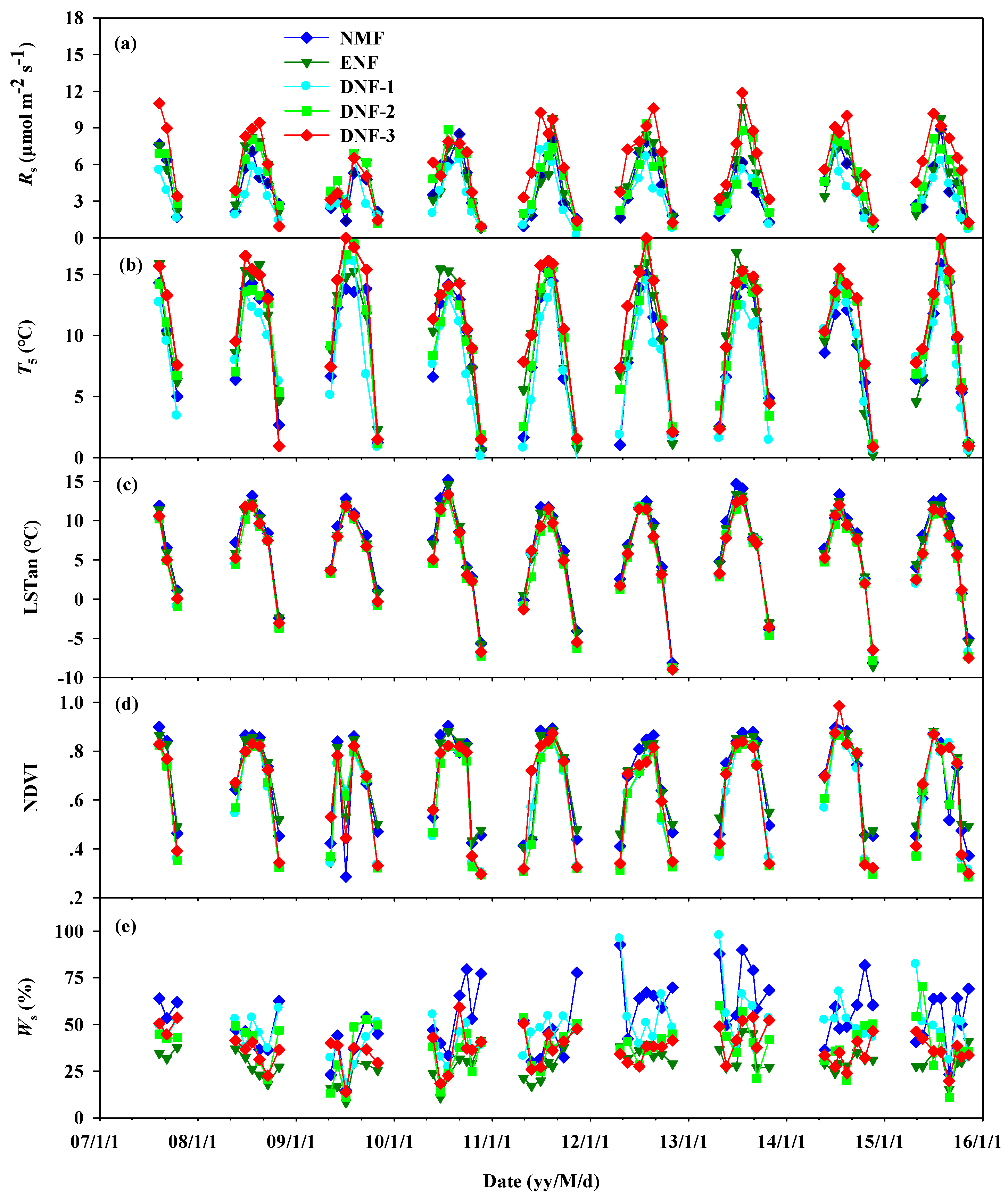
3.1. Seasonal Variations of R_s

Similar to the seasonal variations of T_s and NDVI, R_s showed an obvious seasonal pattern during the study period (Figure 1). The maximum R_s usually appeared at the mid-growing season and corresponded to the maximum T_s and NDVI values, except for one in July of 2009, which corresponded to the lowest W_s recorded during the whole experiment period (Figure 1). One-way ANOVA result illustrated that among the five sites, DNF-3 exhibited the highest R_s, DNF-1 showed the least R_s, and the difference of the average R_s varied among the sites (

Table 3. Mean and coefficient of variation (CV, %) of soil respiration (R_s, μmol CO₂ m⁻² s⁻¹), soil temperature at the 5-cm depth (T₅, °C), land surface temperature (LST_ad and LST_an, °C), normalized difference vegetation index (NDVI), and soil water content at 0 to 10 cm (W_s, %) at the five sites during measurement.

Site Code	Rs		T5		LSTad		LSTan		NDVI		Ws
	Mean	CV	Mean	CV	Mean	CV	Mean	CV	Mean	CV	Mean	CV
NMF	4.24 ± 2.27 ab	53.62	9.33 ± 4.71 ab	50.49	15.21 ± 4.85 a	31.92	6.71 ± 5.89 a	87.77	0.68 ± 0.19 a	28.34	54.19 ± 17.20 e	31.74
ENF	4.76 ± 2.54 b	53.48	10.18 ± 4.96 ab	48.72	15.08 ± 4.72 a	31.27	6.27 ± 5.73 a	91.41	0.69 ± 0.17 a	24.35	29.62 ± 8.32 a	28.09
DNF-1	3.57 ± 1.94 a	54.36	8.45 ± 4.61 a	54.62	14.55 ± 4.99 a	34.29	5.30 ± 5.69 a	107.24	0.62 ± 0.20 a	32.88	48.57 ± 14.26 c	29.37
DNF-2	4.95 ± 2.39 b	48.33	10.20 ± 4.63 ab	45.38	14.54 ± 4.98 a	34.26	5.22 ± 5.74 a	109.83	0.62 ± 0.21 a	34.00	38.29 ± 12.31 b	32.13
DNF-3	6.11 ± 2.94 c	48.20	11.08 ± 5.03 b	45.44	15.13 ± 4.73 a	31.26	5.67 ± 5.72 a	100.82	0.65 ± 0.21 a	31.91	37.50 ± 9.50 b	25.34
All	4.73 ± 2.57	54.15	9.85 ± 4.84	49.14	14.90 ± 4.83	31.79	5.84 ± 5.74	97.77	0.65 ± 0.20	31.75	41.64 ± 15.35	38.97

Data are means ± standard deviations (n = 58). Values in the same column followed by the different letters are significantly different (p < 0.05) based on the Duncan test.

).

T₅ and LST_an exhibited a similar seasonal trend (Figure 1), with a maximum in summer and minimum at the start and end of the growing season. T₅ at DNF-1 was significantly lower (p < 0.05) than at DNF-3, but this was not significantly different (p > 0.05) than at sites NMF, ENF, and DNF-2. However, LST_ad and LST_an were not characterized with a significant difference (p > 0.05) among the five sites (Table 3). Additional analysis indicated that the correlations between the T_s values measured at different depths and all of the LST values were all highly significant (

Table 4. Pearson correlation coefficients (r) among four land surface temperatures (LST) and in situ measured temperatures (T_s) at the five sites during the measurement.

Temperature	NMF			ENF			DNF-1			DNF-2			DNF-3
	T5	T10	T15	T5	T10	T15	T5	T10	T15	T5	T10	T15	T5	T10	T15
LSTan	0.88	0.86	0.82	0.92	0.90	0.87	0.90	0.90	0.85	0.91	0.89	0.85	0.92	0.90	0.89
LSTtn	0.89	0.87	0.83	0.91	0.89	0.87	0.89	0.89	0.83	0.89	0.87	0.83	0.91	0.89	0.88
LSTtd	0.73	0.69	0.62	0.83	0.79	0.74	0.73	0.70	0.61	0.72	0.68	0.62	0.77	0.73	0.69
LSTad	0.68	0.64	0.58	0.74	0.71	0.65	0.72	0.68	0.59	0.69	0.65	0.59	0.74	0.70	0.65

T₅, T₁₀, and T₁₅ is soil temperature (°C) at a depth of 5, 10, and 15 cm, respectively. LST_td and LST_tn is the daytime and nighttime land surface temperature observed by the Moderate Resolution Imaging Spectroradiometer (MODIS) onboard Terra satellites, respectively. LST_ad and LST_an is the daytime and nighttime land surface temperature observed by MODIS onboard Aqua satellites, respectively. The correlation was all significant at the 0.01 level (n = 58).

). Furthermore, the correlations between T_s with nighttime LSTs (LST_tn and LST_an) were significantly stronger than that between T_s with daytime LSTs (LST_ad and LST_td), indicating that for an R_s estimation, the nighttime LST values were better than the daytime LST values. Additionally, among the three depth T_s values, T₅ had the best correlation between the T_s values and LST values.

W_s at the five sites showed a large temporal fluctuation with the occurrence of precipitation events during the measurement. W_s was above 50% of the water holding capacity (WHC) except for in July 2009 (Figure 1). There was a significant difference observed in the average W_s among the sites except for between DNF-2 and DNF-3 (p < 0.05). Among the five sites, the NDVI values did not have a significant difference (p > 0.05), as they ranged from 0.62 ± 0.20 to 0.68 ± 0.19, with a seasonal coefficient of variation (CV) of 24.35 through 34.00% (Table 3). The maximum NDVI typically occurred in the mid-growing period, except for one occasion in July of 2009 (Figure 1), which corresponded exactly to the least W_s (Figure 1).

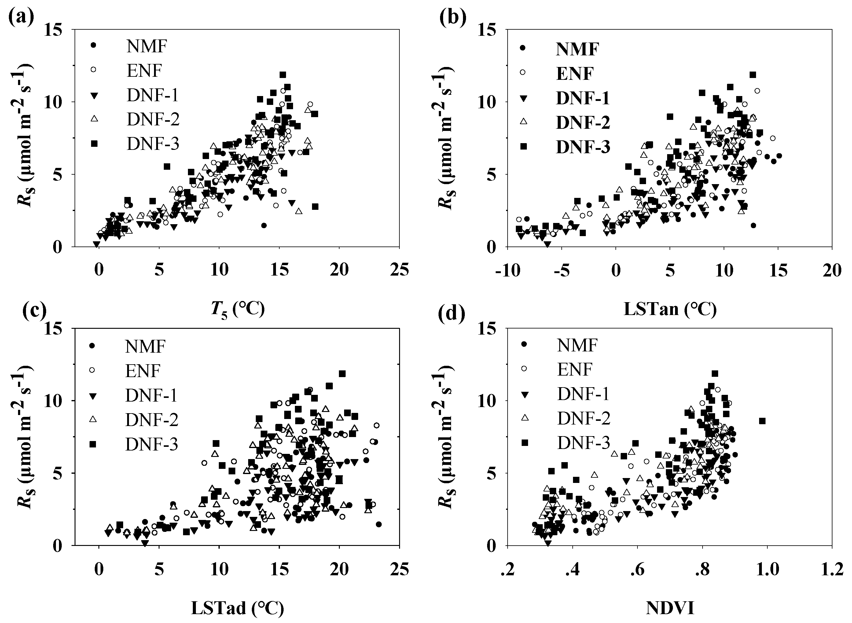
3.2. Correlations between R_s and T_s and LST

The correlations between R_s and the temperatures, including three T_s values and nine MODIS LST values, were all highly significant for each site (

Table 5. Results of the statistical analysis of the fitted Equations (1) and (2) relating soil respiration to temperatures on the five sites for all measured data during the measurement.

Model	Temperature	NMF		ENF		DNF-1		DNF-2		DNF-3
		R2	RMSE	R2	RMSE	R2	RMSE	R2	RMSE	R2	RMSE
Equation (1)	T5	0.74	1.25	0.79	1.34	0.76	1.14	0.77	1.53	0.74	2.01
	T10	0.74	1.25	0.77	1.35	0.72	1.21	0.76	1.49	0.71	2.03
	T15	0.74	1.22	0.76	1.32	0.68	1.23	0.73	1.48	0.67	2.08
	LSTan	0.64	1.50	0.73	1.54	0.79	1.13	0.74	1.48	0.71	1.97
	LSTnightav	0.65	1.46	0.73	1.54	0.78	1.17	0.72	1.55	0.70	2.03
	LSTtn	0.63	1.48	0.69	1.63	0.76	1.26	0.67	1.68	0.67	2.16
	LSTtav	0.57	1.56	0.68	1.73	0.70	1.36	0.64	2.01	0.67	2.20
	LSTav	0.56	1.61	0.67	1.76	0.72	1.34	0.65	2.00	0.67	2.19
	LSTaav	0.53	1.70	0.64	1.85	0.71	1.36	0.62	2.03	0.65	2.22
	LSTtd	0.44	1.83	0.59	1.98	0.55	1.62	0.49	2.03	0.56	2.53
	LSTdayav	0.41	1.90	0.54	2.08	0.58	1.63	0.48	2.09	0.53	2.57
	LSTad	0.35	2.02	0.44	2.25	0.54	1.68	0.41	2.19	0.47	2.65
Equation (2)	T5	0.74	1.24	0.80	1.32	0.78	1.05	0.81	1.40	0.77	1.88
	T10	0.75	1.24	0.79	1.33	0.74	1.12	0.79	1.37	0.75	1.90
	T15	0.75	1.21	0.77	1.30	0.70	1.15	0.75	1.38	0.70	1.96
	LSTan	0.62	1.51	0.71	1.56	0.79	1.09	0.75	1.42	0.74	1.85
	LSTnightav	0.63	1.46	0.72	1.54	0.80	1.10	0.74	1.47	0.74	1.89
	LSTtn	0.62	1.46	0.70	1.58	0.78	1.17	0.71	1.57	0.71	1.98
	LSTtav	0.56	1.59	0.69	1.70	0.72	1.31	0.66	1.96	0.69	2.08
	LSTav	0.55	1.63	0.67	1.74	0.73	1.29	0.66	1.95	0.69	2.08
	LSTaav	0.53	1.69	0.64	1.81	0.72	1.31	0.64	1.99	0.67	2.12
	LSTtd	0.43	1.84	0.60	1.94	0.56	1.57	0.51	1.98	0.58	2.42
	LSTdayav	0.42	1.89	0.56	2.03	0.59	1.57	0.51	2.03	0.56	2.47
	LSTad	0.38	1.98	0.48	2.19	0.56	1.62	0.45	2.13	0.51	2.56

R² is the coefficient of determination; and RMSE (μmol CO₂ m⁻² s⁻¹) is the root mean square error. T₅, T_10, and T₁₅ is soil temperature (°C) at a depth of 5, 10, and 15 cm, respectively. LST_td and LST_tn is the daytime and nighttime land surface temperature observed by MODIS onboard Terra satellites, respectively. LST_tav is the mean of LST_td and LST_tn. LST_ad and LST_an is the daytime and nighttime land surface temperature observed by MODIS onboard Aqua satellites, respectively. LST_aav is the mean of LST_ad and LST_an. LST_av is the mean of LST_td, LST_tn, LST_ad, and LST_an. LST_dayav is the mean of LST_ad and LST_td, LST_nightav is the mean of LST_an and LST_tn. The correlations were all significant at the 0.01 level (n = 58).

, Figure 2), indicating that both T_s and LST values could be used to predict R_s. Furthermore, with the R² and RMSE values of the fitted equations, the T₅ equation was the best one using R_s with T_s at the five sites, and LST_an was the best using LST (Table 5, Table S1).

3.3. Correlations between R_s and VIs

The correlations between the R_s and the three VI values were all significant at the 0.01 level for each site. The exponential and linear functions performed comparably in describing the dependency of R_s on the VI values for the five study sites (

Table 6. Results of statistical analysis relating soil respiration to VIs at the five sites for all measured data during measurement ^a.

Model	VI	NMF		ENF		DNF-1		DNF-2		DNF-3
		R2	RMSE	R2	RMSE	R2	RMSE	R2	RMSE	R2	RMSE
Equation (3)	NDVI	0.76	1.17	0.68	1.46	0.72	0.98	0.74	1.17	0.71	1.65
	EVI	0.65	1.44	0.63	1.70	0.65	1.37	0.63	1.65	0.61	2.03
	CIgreen edge	0.66	1.49	0.54	1.76	0.57	1.63	0.60	1.71	0.60	2.11
Equation (4)	NDVI	0.73	1.18	0.66	1.48	0.72	1.02	0.76	1.17	0.71	1.55
	EVI	0.66	1.32	0.60	1.59	0.65	1.13	0.64	1.42	0.63	1.77
	CIgreen edge	0.70	1.23	0.60	1.60	0.66	1.12	0.69	1.33	0.71	1.55

^a VIs are vegetation indices. NDVI is the normalized difference vegetation index, EVI is the enhanced vegetation index, CI_{green edge} is the green chlorophyll index. R² is the coefficient of determination, and RMSE (μmol CO₂ m⁻² s⁻¹) is the root mean square error. The correlations were all significant at the 0.01 level (n = 58).

). Furthermore, NDVI consistently exhibited a better correlation (with the highest R² and the lowest RMSE) with R_s than the other two VI values at all sites. Therefore, in the following analysis, we selected NDVI to represent the R_s response to GPP at the seasonal time scale.

3.4. Combined Correlations between R_s and T_s (or LST) and NDVI

When T₅ (or LST_an) and NDVI were integrated into one of the six two-variable models (Equations (5)–(10)), the results showed that each of the fitted equations could be used to precisely predict R_s from T₅ (or LST_an) and NDVI variables (

Table 7. Fitting statistics for the respiration models at the five sites for all measured data from during the measurement.

Equation	NMF			ENF			DNF-1			DNF-2			DNF-3
	R2	RMSE	AIC	R2	RMSE	AIC	R2	RMSE	AIC	R2	RMSE	AIC	R2	RMSE	AIC
Soil temperature at 5 cm depth
Rs = a × eb×T	0.74	1.25	29.59	0.79	1.34	37.67	0.76	1.14	19.19	0.77	1.53	53.68	0.74	2.01	85.13
Rs = Rref × e(b(1/56.02−1/(T+46.02)))	0.74	1.24	28.89	0.80	1.32	36.27	0.78	1.05	10.10	0.81	1.40	43.10	0.77	1.88	77.06
Soil temperature at 5 cm depth and NDVI
Rs = a + b × T × VI	0.82	0.96	−1.21	0.79	1.16	20.74	0.80	0.85	−14.18	0.79	1.10	15.08	0.77	1.51	51.47
Rs = a + b × T + c × VI	0.80	1.02	8.21	0.77	1.21	27.75	0.78	0.91	−5.40	0.80	1.08	14.39	0.76	1.52	54.79
Rs = a × e(b×T+c×VI)	0.84	1.10	17.24	0.84	1.17	23.81	0.79	0.90	−6.01	0.81	1.18	25.67	0.78	1.57	58.38
Rs = a × eb×T × VIc	0.85	1.10	17.30	0.84	1.17	24.03	0.79	0.91	−5.15	0.82	1.18	24.87	0.79	1.56	57.64
Rs =Rref × e((b(1/56.02−1/(T+46.02)))+c×VI)	0.84	1.10	16.71	0.85	1.16	23.22	0.80	0.88	−8.32	0.84	1.16	22.86	0.81	1.55	56.89
Rs =Rref × e((b(1/56.02−1/(T+46.02))) × VIc	0.85	0.96	1.36	0.85	1.16	23.55	0.80	0.90	−6.63	0.84	1.16	23.24	0.81	1.55	57.06
Nighttime LST from Aqua MODIS
Rs = a × eb×LST	0.64	1.50	50.92	0.73	1.54	54.19	0.79	1.13	18.00	0.74	1.48	49.17	0.71	1.97	82.56
Rs = Rref × e(b(1/56.02−1/(LST+46.02)))	0.62	1.51	52.13	0.71	1.56	55.94	0.79	1.09	13.86	0.75	1.42	44.28	0.74	1.85	75.11
Nighttime LST from Aqua MODIS and NDVI
Rs = a + b × LST × VI	0.71	1.22	26.91	0.71	1.37	40.37	0.74	0.97	0.71	0.71	1.28	32.94	0.70	1.66	63.04
Rs = a + b × LST + c × VI	0.75	1.12	18.96	0.72	1.34	39.70	0.75	0.97	2.58	0.77	1.15	22.21	0.74	1.57	58.03
Rs = a × e(b×LST+c×VI)	0.81	1.11	18.56	0.81	1.31	37.76	0.81	0.98	3.99	0.79	1.20	27.43	0.77	1.64	63.53
Rs = a × eb×LST × VIc	0.81	1.11	17.80	0.80	1.32	38.26	0.81	1.00	5.54	0.79	1.20	27.28	0.77	1.61	61.37
Rs =Rref × e((b(1/56.02−1/(LST+46.02)))+c×VI)	0.81	1.11	17.81	0.81	1.30	36.65	0.82	0.95	−0.38	0.81	1.17	24.70	0.79	1.60	60.20
Rs =Rref × e((b(1/56.02−1/(LST+46.02))) × VIc	0.82	1.11	17.60	0.80	1.31	37.55	0.82	0.97	2.56	0.81	1.19	26.08	0.79	1.59	59.75

R² is the coefficient of determination, RMSE (μmol CO₂ m⁻² s⁻¹) is the root mean square error, and AIC is a version of Akaike’s information criterion. T₅ is soil temperature at the 5-cm depth. LST_an is the nighttime land surface temperature from Aqua MODIS. VI is the normalized difference vegetation index (NDVI). All relationships were statistically significant at p < 0.01 (n = 58).

). Furthermore, in comparison with the one-dimensional equation (Equations (1)–(4); Table 5 and Table 6), two-variable models (Table 7) were better for all five sites based on the value of RMSE and AIC. According to the model performance indicators (R², RMSE, and AIC), the performances of the fitted T₅–NDVI models were very similar to the fitted LST_an–NDVI model, due to the fact that with the independent t test for the R², RMSE, and AIC values between the R_s to T₅ and NDVI model and the R_s to LST and NDVI model, except for the R², demonstrated a significant difference. However, it was not the case in RMSE and AIC.

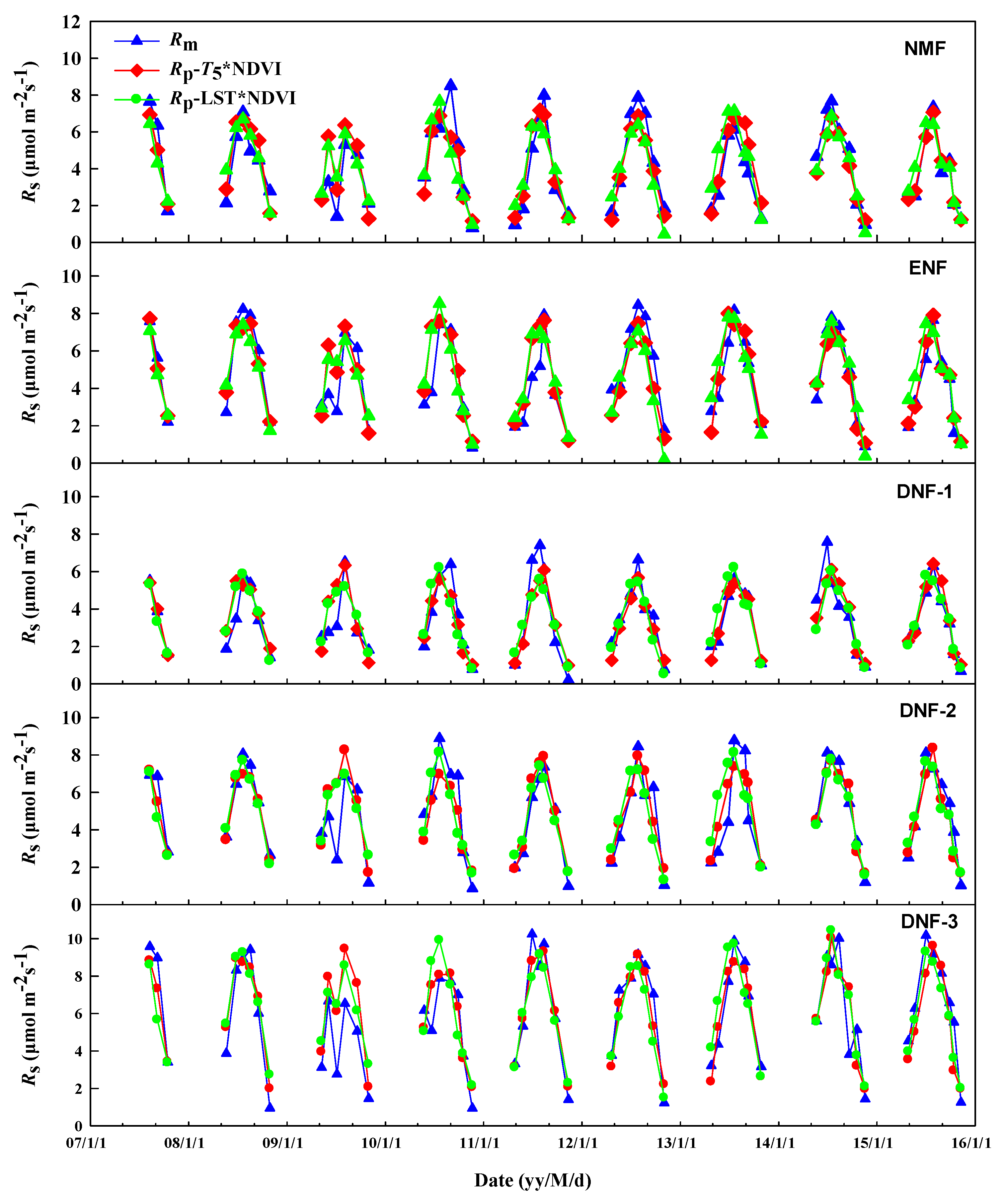
3.5. Modeled Soil Respiration Validation

The results obtained from the leave one out cross-validation are shown in

Table 8. The leave one out cross-validation statistics for the respiration models of the five sites during the measurement.

Equation	NMF			ENF			DNF-1			DNF-2			DNF-3
	R2	RMSE	EF	R2	RMSE	EF	R2	RMSE	EF	R2	RMSE	EF	R2	RMSE	EF
Soil temperature at 5 cm depth
Rs = a × eb×T	0.76	1.36	0.48	0.79	1.25	0.31	0.78	1.19	0.27	0.77	1.50	0.21	0.74	1.88	−0.32
Rs = Rref × e(b(1/56.02−1/(T+46.02)))	0.76	1.37	0.49	0.79	1.25	0.33	0.80	1.10	0.45	0.78	1.37	0.36	0.76	1.73	−0.05
Soil temperature at 5 cm depth and VI
Rs = a = b × T × VI	0.81	1.18	0.63	0.87	1.01	0.63	0.84	0.87	0.70	0.84	1.09	0.66	0.84	1.40	0.47
Rs = a = b × T + c × VI	0.79	1.26	0.59	0.81	1.11	0.53	0.80	1.00	0.60	0.81	1.11	0.64	0.80	1.58	0.31
Rs = a × e(b×T+c×VI)	0.81	1.20	0.60	0.83	1.10	0.56	0.80	1.05	0.53	0.82	1.25	0.48	0.78	1.71	−0.06
Rs = a × eb×T × VIc	0.81	1.20	0.60	0.87	1.03	0.61	0.83	0.97	0.59	0.81	1.24	0.50	0.78	1.66	0.06
Rs =Rref × e((b(1/56.02−1/(T+46.02)))+c×VI)	0.81	1.21	0.61	0.85	1.07	0.58	0.83	0.95	0.62	0.82	1.21	0.53	0.79	1.64	0.06
Rs =Rref × e((b(1/56.02−1/(T+46.02))) × VIc	0.81	1.21	0.61	0.86	1.04	0.61	0.83	0.95	0.62	0.82	1.21	0.53	0.79	1.62	0.12
Nighttime LST from Aqua MODIS
Rs =a × eb×LST	0.67	1.58	0.35	0.66	1.49	0.22	0.71	1.15	0.46	0.69	1.41	0.44	0.67	1.87	0.00
Rs = Rref × e(b(1/56.02−1/(LST+46.02)))	0.66	1.60	0.37	0.64	1.50	0.26	0.72	1.09	0.54	0.71	1.37	0.48	0.71	1.77	0.15
Nighttime LST from Aqua MODIS and VI
Rs = a = b × LST × VI	0.73	1.40	0.49	0.76	1.24	0.49	0.77	1.00	0.62	0.75	1.19	0.59	0.78	1.58	0.34
Rs = a = b × LST = c × VI	0.74	1.37	0.53	0.79	1.16	0.55	0.76	1.00	0.61	0.77	1.55	0.38	0.80	1.57	0.41
Rs = a × e(b×LST+c×VI)	0.76	1.31	0.54	0.82	1.20	0.50	0.76	1.03	0.58	0.77	1.16	0.61	0.76	1.68	0.23
Rs = a × eb×LST × VIc	0.76	1.33	0.53	0.81	1.13	0.58	0.76	1.04	0.58	0.77	1.16	0.61	0.77	1.63	0.31
Rs =Rref × e((b(1/56.02−1/(LST+46.02)))+c×VI)	0.77	1.30	0.55	0.81	1.15	0.57	0.78	0.98	0.63	0.78	1.12	0.64	0.76	1.65	0.25
Rs =Rref × e((b(1/56.02−1/(LST+46.02))) × VIc	0.76	1.32	0.55	0.81	1.15	0.57	0.77	0.99	0.62	0.78	1.14	0.63	0.77	1.60	0.34

R² is the coefficient of determination, RMSE is the root mean square error, and EF is the modeling efficiency. The correlations were all significant at the 0.01 level (n = 58).

. In contrast to the cross -validation statistical result of the one-dimensional equation, the R² and EF of the two-dimensional equations increased, and RMSE decreased. This further confirmed our conclusion that the application of the two-dimensional equations of T₅–NDVI (or LST_an–NDVI) is better than the one-dimensional equations of T₅ (or LST_an) in predicting R_s at a seasonal scale. Furthermore, the cross-validated statistics of the models driven by LST_an or LST_an–NDVI were slightly lower than those of the models of the in situ measured T₅ or T₅–NDVI.

The modeled R_s closely resembled the seasonal patterns of the measured R_s (Figure 3). R_s increased quickly after the start of the growing season and maximized in the summer months and then underwent an evident decrease since autumn. An obvious overestimation that occurred on 5 July 2009 at the five forest sites reduced the evaluation accuracy of the cross-validation because of summer drought. When 2009 was excluded from the model validation, the R² and EF of the cross-validation increased and RMSE decreased compared with that including all measured data for one of the five sites (Table S2). Moreover, underestimation was observed after raining or the middle growing period.

4. Discussion

4.1. The Impact of Temperature on R_s

The LST data from MODIS products can potentially be used as a measure of temperature [17]. At our study site, MODIS Terra and Aqua LST values were all significantly correlated with the observed T_s (Table 4). When comparing the correlation between nighttime LST values and in situ observed T_s values with that of the correlation of daytime LST and in situ observed T_s, the better nighttime correlation could be attributed to both the absence of a solar radiation effect on the thermal infrared signal at night [26] and the influence of vegetation during daytime [27]. During the daytime, dense vegetation may increase the conversion of solar incident energy into latent heat, and thus cool the surface through evapotranspiration. During the nighttime, vegetation exerts a negligible effect on the correlation between surface air temperature and nighttime LST [19,27].

In our study, we found that the MODIS LST data could be used to establish models estimating R_s, as an alternative to T_s. Our results also show that nighttime LST data were usually better correlated with R_s than daytime LST, as indicated by the performance of the exponential functions and the Arrhenius-type functions (Table 5). It was concluded that nighttime LST was the optimal predictor for estimating R_s. This might be attributed to the nighttime LST values, indicating the baseline temperature regulates plant phenology [17].

Our result is consistent with previous studies [19,20,27]. For example, in a Canadian boreal black spruce stand, Wu et al. [20] reported that nighttime LST showed a greater potential in explaining variations in R_s than daytime LST, referring to the fact that nighttime LST is more resistant to various residual noise components. Huang et al. [19] suggests that an accurate estimation of R_s could be inferred with Terra MODIS LST using either nighttime LST or the mean of daytime and nighttime LST as the independent variable in regression equations.

4.2. Vegetation Index as a Driver of Rs

We identified that R_s was correlated with three kinds of VIs (i.e., NDVI, EVI, and CI_{green edge}). Others observed the same phenomenon [28,29]. This result suggests that the spectral vegetation indexes from remote sensing can be used in the prediction model of R_s. There was a consistently stronger correlation between R_s and NDVI than the correlation between R_s and EVI or CI_{green edge} for the five forest sites (Table 6), which was not consistent with others. For example, at a maize and a winter wheat field, Huang et al. [28] reported that EVI or CI_{red edge} consistently exhibited a better correlation with R_s than NDVI, which was attributed to NDVI showing less of a seasonal variation than EVI and CI_{red edge}, particularly when the green leaf area index (GLAI) was greater than 3. Huete et al. [22] also reported that NDVI tends to saturate at high vegetation densities, and is highly sensitive to differences in background reflectance. Conversely, EVI and CI_{red edge} improved the canopy background correction and are more sensitive than NDVI to variation in dense vegetation. In our study, the vegetation types of the five study sites are all cold temperate coniferous forests, and the in situ measured monthly LAI ranged from 1.85 to 4.22, 3.08 to 4.77, 1.27 to 2.96, 0.80 to 2.27, and 0.74 to 2.84 from April 2015 to October 2015 at the NMF, ENF, DNF-1, DNF-2, and DNF-3 sites, respectively (Figure 4). Compared with the other reports, our study sites illustrated a sparse vegetation region, and a lower vegetation index. Therefore, NDVI consistently exhibited a better correlation with R_s than the other two VI values. Vegetation indexes at the ENF site are not as well correlated with R_s than that at other sites. This may be attributed to the fact that the ENF site is an evergreen needle leaf forest and the coefficient of variation of its vegetation coverage within a year is the least one among the five sites.

4.3. Spatial Scale of the Data

The spatial scales of the data for analysis in our study are different. R_s, T_s, and W_s measurements at each site were carried out in an area of approximately 400 m², and their values were averaged. However, each pixel of the MODIS 8-day surface reflectance and 8-day LST products represents an area of 500 m × 500 m and 1000 m × 1000 m, respectively. Therefore, the MODIS products (i.e., VI and LST values) are not necessarily consistent with in situ measured data (i.e., R_s, T_s, and W_s) in the spatial scale. Despite that, we found that the MODIS LST and the measured T_s showed a consistent seasonal variation pattern (Figure 1). In addition, a Pearson correlation analysis showed that the MODIS LST values and the measured T_s (i.e., T₅, T₁₀, and T₁₅) were all significantly correlated at the 0.01 level for the five forest sites (Table 4). Huang et al. [3] observed the similar pattern. In our study site in a sub-alpine meadow, it is feasible to predict both R_s with MODIS products and the in situ measured soil temperature [30]. Recently, MODIS data have also been confirmed to estimate ecosystem respiration on the global scale [31]. Therefore, MODIS LST may be identified as a proxy indicator of T_s to estimate R_s.

4.4. Limitation of the Study

The models driven by remote sensing data (i.e., LST_an and NDVI) performed well in R_s estimation at the current five forest sites; however, several limitations are listed below:

We focused our study on the growing season of five temperate coniferous forest sites; therefore, the model’s performance in the non-growing season still needs to be evaluated. The previous study also reported that the factors influencing R_s in different phenological phases may be different. For example, Huang et al. [3] found the models driven by mean LST and root zone soil moisture could explain most of the non-growing season’s variations in R_s at a deciduous forest site. The models including the mean LST, root zone soil moisture, and EVI exhibited a high accuracy for R_s estimation in early and late-growing periods. However, in the mid-growing period, the model entirely dependent on mean LST, root zone soil moisture, and EVI may exhibit a lower explanation capacity for seasonal variation of R_s than the model driven by in situ measured T_s at the 4 cm depth, W_s at the 10 cm depth, and gross primary productions.

Because the W_s factor was not explicitly included in the prediction models of R_s, the satellite-driven model may provide a relatively poor R_s estimation under severe drought and raining pulse conditions, as we observed. Throughout the nine-year study period, W_s was below 50% of WHC only in the measurement on July 2009, where the corresponding R_s was also uniformly lower than that in the same period in other years at the five study sites. An obvious overestimation of R_s was also found on 5 July 2009 (Figure 3). The overestimation may be attributed to the model being based only on LST_an and NDVI and not including the effect of W_s on R_s. In order to further explore the impact of W_s on the performances of models only based on T₅ or LST_an, a regression analysis was conducted using logarithmic and parabolic models. The result showed a mean W_s from May to October (MAW) or mean W_s from May to July (MTW) was significantly correlated with the R² of the exponential model of T₅ or LST_an to R_s (Table S3) except the DNF-2 and DNF-3 sites. The correlation with MTW was better than with MAW in most cases, indicating that the performance of the R_s model based on T₅ or LST_an was influenced by W_s. Wu et al. [20] also reported that the R_s model based on the data of MODIS LST and NDVI is affected by the soil water amount.

Remotely sensed LST data lack observations for cloud-covered areas [32]. The soil respiration measurement includes both sunny and cloudy days. Moreover, in our study, VI and LST values corresponding to the R_s measurement days were from the two consecutive 8-day composites by linear interpretation. Consequently, information extraction errors from remote sensing data may introduce errors into R_s prediction.

The value of R_s is also influenced by soil texture, substrate quantity, and quality [33]. These factors were not incorporated into our model, however in future studies these factors may improve the accuracy of the R_s models and should be investigated further.

5. Conclusions

We investigated the feasibility of estimating R_s using solely MODIS product data on five cold temperate coniferous forest sites in the eastern Loess Plateau, China. The results showed that the accuracy of the model based on the observed surface soil temperatures was not significantly different with that of the model based on MODIS-derived nighttime LST values. However, the model using MODIS-derived daytime LST values was significantly different, indicating that nighttime land surface temperatures were the optimum LST for estimating R_s. Between the selected three VI values, NDVI consistently exhibited a better correlation with R_s, compared to EVI and CI_{green edge}. Adding NDVI into the model considering only T_s or nighttime LST significantly improved the simulation accuracy of R_s. The models driven by LST_an and NDVI demonstrated a similar performance to the models considering T₅ and NDVI based on the test of the AIC, R², and RMSE values. Our findings demonstrate that models based entirely on remote sensing data have the potential to predict R_s in the cold temperate coniferous forest sites. Our previous study and other researches at different sites and vegetation types also have confirmed the feasibility of estimating R_s using solely MODIS product data. The present study provides valuable information for the large-scale estimation of R_s in cold temperate deciduous forest ecosystems. It is possible that the use of MODIS data for soil respiration estimation will provide a great convenient way for forest carbon budget calculation at larger scales.

References

1. Raich, J.W.; Potter, C.S.; Bhagawati, D. Interannual variability in global soil respiration, 1980–1994. Glob. Chang. Biol. 2002, 8, 800–812. [Google Scholar] [CrossRef]
2. Richardson, A.D.; Braswell, B.H.; Hollinger, D.Y.; Burman, P.; Davidson, E.A.; Evans, R.S.; Flanagan, L.B.; Munger, J.W.; Savage, K.; Urbanski, S.P.; et al. Comparing simple respiration models for eddy flux and dynamic chamber data. Agric. For. Meteorol. 2006, 141, 219–234. [Google Scholar] [CrossRef]
3. Huang, N.; Gu, L.; Niu, Z. Estimating soil respiration using spatial data products: A case study in a deciduous broadleaf forest in the Midwest USA. J. Geophys. Res. Atmos. 2014, 119, 6393–6408. [Google Scholar] [CrossRef]
4. Deimling, T.; Meinshausen, M.; Levermann, A.; Huber, V.; Frieler, K.; Lawrence, D.M.; Brovkin, V. Estimating the near-surface permafrost-carbon feedback on global warming. Biogeosciences 2012, 9, 649–665. [Google Scholar] [CrossRef] [Green Version]
5. Buchmann, N. Biotic and abiotic factors controlling soil respiration rates in Picea abies stands. Soil Biol. Biochem. 2000, 32, 1625–1635. [Google Scholar] [CrossRef]
6. Davidson, E.A.; Belk, E.; Boone, R.D. Soil water content and temperature as independent or confounded factors controlling soil respiration in a temperate mixed hardwood forest. Glob. Chang. Biol. 1998, 4, 217–227. [Google Scholar] [CrossRef] [Green Version]
7. Li, H.J.; Yan, J.X.; Yue, X.F.; Wang, M.B. Significance of soil temperature and moisture for soil respiration in a Chinese mountain area. Agric. For. Meteorol. 2008, 148, 490–503. [Google Scholar] [CrossRef]
8. Han, C.; Liu, T.; Duan, L.; Zhang, S.; Singh, V.P. Spatio-temporal distribution of soil respiration in dune-meadow cascade ecosystems in the Horqin Sandy Land, China. CATENA 2017, 157, 397–406. [Google Scholar] [CrossRef]
9. Yu, S.; Chen, Y.; Zhao, J.; Fu, S.; Li, Z.; Xia, H.; Zhou, L. Temperature sensitivity of total soil respiration and its heterotrophic and autotrophic components in six vegetation types of subtropical China. Sci. Total Environ. 2017, 607–608, 160–167. [Google Scholar] [CrossRef]
10. Wang, Q.; He, T.; Wang, S.; Liu, L. Carbon input manipulation affects soil respiration and microbial community composition in a subtropical coniferous forest. Agric. For. Meteorol. 2013, 178–179, 152–160. [Google Scholar] [CrossRef]
11. Chen, S.; Huang, Y.; Zou, J.; Shen, Q.; Hu, Z.; Qin, Y.; Chen, H.; Pan, G. Modeling interannual variability of global soil respiration from climate and soil properties. Agric. For. Meteorol. 2010, 150, 590–605. [Google Scholar] [CrossRef]
12. Huang, N.; Wang, L.; Guo, Y.; Hao, P.; Niu, Z. Modeling spatial patterns of soil respiration in maize fields from vegetation and soil property factors with the use of remote sensing and geographical Information System. PLoS ONE 2014, 9, e105150. [Google Scholar] [CrossRef] [PubMed] [Green Version]
13. Luan, J.; Liu, S.; Zhu, X.; Wang, J.; Liu, K. Roles of biotic and abiotic variables in determining spatial variation of soil respiration in secondary oak and planted pine forests. Soil Biol. Biochem. 2012, 44, 143–150. [Google Scholar] [CrossRef]
14. Chen, S.; Zou, J.; Hu, Z.; Chen, H.; Lu, Y. Global annual soil respiration in relation to climate, soil properties and vegetation characteristics: Summary of available data. Agric. For. Meteorol. 2014, 198–199, 335–346. [Google Scholar] [CrossRef]
15. Reichstein, M.; Rey, A.; Freibauer, A.; Tenhunen, J.; Valentini, R.; Banza, J.; Casals, P.; Cheng, Y.; Grünzweig, J.; Irvine, J.; et al. Modeling temporal and large-scale spatial variability of soil respiration from soil water availability, temperature and vegetation productivity indices. Glob. Biogeochem. Cycle 2003, 17, 1104. [Google Scholar] [CrossRef]
16. Zhou, Z.; Zhang, Z.; Zha, T.; Luo, Z.; Zheng, J.; Sun, O.J. Predicting soil respiration using carbon stock in roots, litter and soil organic matter in forests of Loess Plateau in China. Soil Biol. Biochem. 2013, 57, 135–143. [Google Scholar] [CrossRef]
17. Sims, D.A.; Rahman, A.F.; Cordova, V.D.; El-Masri, B.Z.; Baldocchi, D.D.; Bolstad, P.V.; Flanagan, L.B.; Goldstein, A.H.; Hollinger, D.Y.; Misson, L.; et al. A new model of gross primary productivity for North American ecosystems based solely on the enhanced vegetation index and land surface temperature from MODIS. Remote Sens. Environ. 2008, 112, 1633–1646. [Google Scholar] [CrossRef]
18. Gao, Y.; Yu, G.; Li, S.; Yan, H.; Zhu, X.; Wang, Q. A remote sensing model to estimate ecosystem respiration in Northern China and the Tibetan Plateau. Ecol. Model. 2015, 304, 34–43. [Google Scholar] [CrossRef]
19. Huang, N.; Gu, L.; Black, T.A.; Wang, L.; Niu, Z. Remote sensing-based estimation of annual soil respiration at two contrasting forest sites. J. Geophys. Res. Biog. 2015, 120, 2306–2325. [Google Scholar] [CrossRef] [Green Version]
20. Wu, C.; Gaumont-Guay, D.; Black, T.A.; Jassal, R.S.; Xu, S.; Chen, J.M.; Gonsamo, A. Soil respiration mapped by exclusively use of MODIS data for forest landscapes of Saskatchewan, Canada. ISPRS J. Photogramm. Remote Sens. 2014, 94, 80–90. [Google Scholar] [CrossRef]
21. Gamon, J.A.; Field, C.B.; Goulden, M.L.; Griffin, K.L.; Hartley, A.E.; Joel, G.; Peñuelas, J.; Valentini, R. Relationships between NDVI, canopy structure, and photosynthesis in three Californian vegetation types. Ecol. Appl. 1995, 5, 28–41. [Google Scholar] [CrossRef] [Green Version]
22. Huete, A.; Didan, K.; Miura, T.; Rodriguez, E.P.; Gao, X.; Ferreira, L.G. Overview of the radiometric and biophysical performance of the MODIS vegetation indices. Remote Sens. Environ. 2002, 83, 195–213. [Google Scholar] [CrossRef]
23. Gitelson, A.A.; Vina, A.; Ciganda, V.; Rundquist, D.C.; Arkebauer, T.J. Remote estimation of canopy chlorophyll content in crops. Geophys. Res. Lett. 2005, 32, L08403. [Google Scholar] [CrossRef] [Green Version]
24. Lloyd, J.; Taylor, J.A. On the temperature dependence of soil respiration. Funct. Ecol. 1994, 8, 315–323. [Google Scholar] [CrossRef]
25. Migliavacca, M.; Reichstein, M.; Richardson, A.D.; Colombo, R.; Sutton, M.A.; Lasslop, G.; Tomelleri, E.; Wohlfahrt, G.; Carvalhais, N.; Cescatti, A.; et al. Semi-empirical modeling of abiotic and biotic factors controlling ecosystem respiration across eddy covariance sites. Glob. Chang. Biol. 2011, 17, 390–409. [Google Scholar] [CrossRef]
26. Benali, A.; Carvalho, A.C.; Nunes, J.P.; Carvalhais, N.; Santos, A. Estimating air surface temperature in Portugal using MODIS LST data. Remote Sens. Environ. 2012, 124, 108–121. [Google Scholar] [CrossRef]
27. Zhang, W.; Huang, Y.; Yu, Y.; Sun, W. Empirical models for estimating daily maximum, minimum and mean air temperatures with MODIS land surface temperatures. Int. J. Remote Sens. 2011, 32, 9415–9440. [Google Scholar] [CrossRef]
28. Huang, N.; Niu, Z. Estimating soil respiration using spectral vegetation indices and abiotic factors in irrigated and rainfed agroecosystems. Plant Soil 2012, 367, 535–550. [Google Scholar] [CrossRef]
29. Sánchez, M.L.; Ozores, M.I.; López, M.J.; Colle, R.; Torre, B.D.; García, M.A.; Pérez, I. Soil CO2 fluxes beneath barley on the central Spanish plateau. Agric. For. Meteorol. 2003, 118, 85–95. [Google Scholar] [CrossRef]
30. Liang, Y.; Cai, Y.; Yan, J.; Li, H. Estimation of soil respiration by its driving factors based on multi-source data in a sub-alpine meadow in north China. Sustainability 2019, 11, 3274. [Google Scholar] [CrossRef] [Green Version]
31. Ai, J.L.; Jia, G.S.; Epstein, H.E.; Wang, H.S.; Zhang, A.Z.; Hu, Y.H. MODIS-based estimates of global terrestrial ecosystem respiration. J. Geophys. Res. Biog. 2018, 123, 326–352. [Google Scholar] [CrossRef]
32. Crosson, W.L.; Al-Hamdan, M.Z.; Hemmings, S.N.J.; Wade, G.M. A daily merged MODIS Aqua–Terra land surface temperature data set for the conterminous United States. Remote Sens. Environ. 2012, 119, 315–324. [Google Scholar] [CrossRef]
33. Liu, H.S.; Li, L.H.; Han, X.G.; Huang, J.H.; Sun, J.X.; Wang, H.Y. Respiratory substrate availability plays a crucial role in the response of soil respiration to environmental factors. Appl. Soil Ecol. 2006, 32, 284–292. [Google Scholar] [CrossRef]
Figure 1. Seasonal variations in the (a) soil respiration rate (Rs, μmol CO2 m−2 s−1), (b) soil temperature at 5 cm depth (T5, °C), (c) land surface nighttime temperature from MODIS-Aqua (LSTan, °C), (d) normalized difference vegetation index (NDVI), and (e) soil water content at 0 to 10 cm (Ws, %) at the five sites during measurement.
Forests 11 00131 g001
Figure 2. Correlations between soil respiration (Rs, μmol CO2 m−2 s−1) and (a) soil temperature at the 5 cm depth (T5, °C), (b) nighttime land surface temperature from Aqua MODIS (LSTan, °C), (c) daytime land surface temperature from Aqua MODIS (LSTad, °C), and (d) normalized difference vegetation index (NDVI) during the measurement.
Forests 11 00131 g002
Figure 3. Seasonal variations of soil respiration measured (Rm) and predicted (Rp) by model five based on in situ soil temperature and NDVI (RpT5*NDVI) or nighttime LST and NDVI (Rp–LSTan*NDVI) for the five study sites.
Forests 11 00131 g003
Figure 4. The seasonal variations of leaf area index (LAI) from April to October 2015.
Forests 11 00131 g004