Assessing Differences in Competitive Effects Among Tree Species in Central British Columbia, Canada

Abstract

Research Highlights: We investigated the competitive interactions among three tree species (interior Douglas-fir (Pseudotsuga menziesii var. glauca (Beissn.) Franco), interior spruce (Picea glauca [Moench] Voss × Picea engelmannii Engelm.), and lodgepole pine (Pinus contorta Dougl. Ex Loud. var. latifolia Englem.)) in multi-aged stands in central British Columbia, Canada. Background and Objectives: Understanding competitive interactions among tree species in mixed-species stands is fundamental to supporting silvicultural decision-making in such stands. Using the periodic annual basal area increment for single trees as our dependent variable, we investigated whether neighboring trees competed with subject trees independently of species identity. We also examined the differences in single-tree basal area growth among the three conifer species over time under different levels of competition. Materials and Methods: We developed several spatially explicit, single-tree basal area growth models for interior Douglas-fir, interior spruce, and lodgepole pine using data from 16 plots in two blocks of a long-term study (five measurements over a 21-year period) on the response to pre-commercial thinning. We compared these equations to assess whether intraspecific or interspecific competition predominated. We also examined the differences in basal area growth among the three conifer species over time under different levels of competition. Results: We found asymmetrical relationships between the conifer trees and their neighbors for all species, indicating that the main driver limiting growth in these stands is aboveground competition for light. There was evidence of higher intraspecific competition for small (<10.0 cm DBH) interior Douglas-fir in one block. However, there was no general pattern among larger subject trees with respect to the identity of neighborhood competitive effects and the equivalence of neighbors. We observed a higher level of basal area growth over time for interior Douglas-fir than for lodgepole pine and interior spruce, irrespective of the competition intensity and, not surprisingly, the growth rate declined with increasing competition levels for the three species. Conclusions: Our results provide an understanding of how interior Douglas-fir stands will develop over time and information on species interactions that could help forest managers explore different silvicultural options and their effects on individual tree growth in these complex stands.

1. Introduction

Mixed-species forest stands are increasingly gaining attention as studies have highlighted their importance in providing higher levels of ecosystem services and functions [1]. Mixed-species stands may also be more productive and have a higher resistance to biotic and abiotic disturbances [2,3]. Interactions between tree species in such forests may be complex and dynamic due to changes to the environment and resource availability. However, understanding the interaction among species in mixed-species stands is fundamental to supporting managerial decision-making.

Differing interactions among trees (competition (negative), facilitation (neutral or positive), and competitive reduction) are widely described in the literature [2]. Oliver and Larson [4] describe competition as an interaction between trees that results in one individual obtaining a greater share of growth resources (growing space) than another, leading to that individual gaining dominance over the other. Facilitation occurs when the growth and presence of a tree positively influences the growth of another and can occur simultaneously with competition. Competitive reduction indicates lower interspecific competition due to differentiation for resources among two or more species. The three processes are difficult to differentiate and are collectively referred to as complementarity [5], i.e., the effect of a species mixture on growth. The contribution of each process to the total complementarity effect is also difficult to quantify [2]. Environmental conditions play a critical role in determining the direction, effect, and intensity of interactions [6]. For example, under high abiotic stress, interactions shift towards facilitation (as described by the stress-gradient hypothesis) [7].

Several growth models (growth simulators) have been used in the literature to study and evaluate the interactions of mixed-species forest stands. Generally, these simulators are individual-tree-based and spatially explicit. According to Zhao et al. [8], it is preferable to use such an approach in mixed-species stands to describe the mode of competition among individual trees and the association among species, as well as to predict stand development. The identity of neighboring tree species is important in characterizing their competitive effect [8,9].

Competition indices that characterize the degree to which the growing space of a subject tree is shared by its neighbors can help to quantify inter-tree interactions and model individual tree or stand growth [10]. Competition can occur among conspecific individuals (plants of the same species) and hetero-specific individuals (plants of different species), termed intraspecific and interspecific competition, respectively. In stands that are complex in structure and represent a heterogeneous mixture of species, there is strong evidence that interspecific and intraspecific competition differ [8,11]. For example, it has been found in some studies that competitive effects among different species are unequal and asymmetric [8]. In contrast, other studies indicate that all individuals, irrespective of species identity, are functionally equivalent competitors [12,13]. Some studies have found that conspecific neighbors are stronger competitors than hetero-specific neighbors [14,15]. However, von Oheimb et al. [13] found no significant influence of conspecific neighbors on growth, but a strong negative effect of hetero-specific neighbors on growth.

Competition may be unequal for trees of different species, size, and ages. Competitive interactions among trees are either size-symmetric or size-asymmetric [16]. There is a consensus that belowground competition (competition for water and nutrients) is size-symmetric, where the access of individual trees to resources is directly proportional to their size. In contrast, competition for aboveground resources (competition for light) is size-asymmetric, where larger trees obtain a disproportionate amount of available resources and suppress the growth of smaller individuals. Size-asymmetric competition by neighboring trees can increase growth variability within stands over time [17], whereas size-symmetric competition evenly reduces individual tree growth below potential levels [18]. In mixed-species stands, both size-symmetric and size-asymmetric competition are likely to be present. Competition models often assume that aboveground conditions also adequately describe belowground conditions and processes [19].

Although there are a number of studies on neighborhood effects on the growth and survival of individual tree species [8,13,20], neighborhood effects on individual tree growth may vary considerably due to tree species composition, climatic conditions, and stand development history. Stands in the dry-belt, uneven-aged interior Douglas-fir (Pseudotsuga menziesii var. glauca (Beissn.) Franco) region of British Columbia, Canada (BC), are noted for their complex structures due to a history of disturbances from partial cutting, insects, and fire [21]. These complexities have rendered crown closure, canopy layering, and size–age relationships highly variable from one stand to another and often within any one stand [22]. In these stands, interior Douglas-fir grows in pure stands or in mixtures with interior spruce (Picea glauca [Moench] Voss × Picea engelmannii Engelm.) and other species [23]. Therefore, these forests may have their own mode of competition and it may be important to determine whether the species identity of neighboring trees improves the ability of spatially explicit models to account for growth variability. Additionally, changes in the stand structure, due to stochastic disturbance events or partial harvesting, could lead to changes in the neighborhood competition effects over time.

In this study, spatially explicit, single-tree basal area growth models were developed using data from a long-term study (five measurements over a 21-year period) on the response to pre-commercial thinning in the central interior of BC. These models were used to (i) investigate whether neighboring trees compete with a subject tree independently of species identity, and (ii) examine the differences in basal area growth among the three conifer tree species present in the study area (interior Douglas-fir, interior spruce, and lodgepole pine (Pinus contorta Dougl. Ex Loud. var. latifolia Englem.) over time under different degrees of competition. To address these objectives, we fitted a nonlinear mixed-effect basal area growth model for a subject tree, incorporating tree size (DBH) and the competition effect of neighboring trees, irrespective of species (i.e., all species are treated as equivalent competitors). Subsequently, we partitioned the competitive effects of neighbors into different species or species groups to allow us to incorporate potential differences in competitive relationships among species.

2. Materials and Methods

2.1. Study Site and Data

We examined 21 years of growth records from a pre-commercial thinning (spacing) study in the dry cool subzone of the Interior Douglas-fir zone (IDFdk) of the Biogeoclimatic Ecosystem Classification (BEC) system in British Columbia, Canada [24]. The study was located in the Knife Creek Unit of the University of British Columbia’s Alex Fraser Research Forest (52°3′ N, 121°52′ W). The Knife Creek Unit covers an area of approximately 3500 ha [25], situated on the Fraser plateau approximately 27 km east of Williams Lake, in the south-central part of BC (Figure 1). The Fraser plateau has an average elevation of about 1000 m, a mean daily temperature of 4.2 °C, and an average annual precipitation of 450 mm [24].

During the summers of 1989 and 1990, three blocks (B, C, and D), of approximately 40 hectares each, were selected for this experiment. Block B is quite dry, Block C is more mesic, and Block D is the moistest of the sites and is transitional to the Sub-Boreal Spruce (SBS) BEC zone. The stands were logged during the 1950s and 1960s to a diameter limit of approximately 25.4 cm, although a few of the larger trees were not harvested. Block B was dominated by interior Douglas-fir (>80% by basal area), with the remaining basal area consisting of lodgepole pine and a small percentage (<0.5%) of trembling aspen (Populus tremuloides Michx). Block C was also dominated by Douglas-fir (>60% basal area). Lodgepole pine varied among the plots (0%–26.5% basal area) and there was a small interior spruce component (less than 5% by basal area). The remaining basal area was comprised of white birch (Betula papyrifera Marsh.) and trembling aspen. Block D was dominated by mixtures of Douglas-fir, spruce, and lodgepole pine (together accounting for more than 80% of the basal area). The remaining basal area was comprised of aspen and white birch. For this analysis, plots from Blocks C and D (16 in total) were used because a sufficient species mixture was present to enable the assessment of interspecific competition in terms of the basal area growth of the three conifer species (hereafter referred to as interior Douglas-fir (FD), interior spruce (SX), and lodgepole pine (PL)) (

Table 1. Summary statistics (number of trees (n), and mean, minimum (Min), and maximum (Max) diameter at breast height (DBH)) by block, measurement year, and tree species or species group.

Year	Tree Species	Block C				Block D
			DBH (cm)				DBH (cm)
		n	Mean	Min	Max	n	Mean	Min	Max
1993	Douglas-fir	861	8.7	0.2	37.6	725	9.0	0.3	51.5
	Spruce	17	12.4	2.0	23.5	237	10.1	1.0	27.5
	Lodgepole pine	80	11.7	0.6	31.1	69	15.0	5.5	41.1
	Broadleaf (aspen and birch)	140	6.5	0.3	20.2	74	8.4	0.3	46.1
1997	Douglas-fir	862	9.2	0.2	38.5	716	9.6	0.6	52.5
	Spruce	17	13.7	3.1	25.5	225	10.8	0.9	28.5
	Lodgepole pine	76	13.0	0.4	32.2	68	17.1	5.6	41.5
	Broadleaf (aspen and birch)	119	7.0	0.3	21.0	76	7.3	0.2	47.0
2004	Douglas-fir	840	10.3	0.1	39.5	679	10.7	0.3	54.2
	Spruce	17	15.5	4.8	27.3	196	12.2	1.4	30.0
	Lodgepole pine	65	11.9	0.4	30.9	64	13.4	5.7	32.4
	Broadleaf (aspen and birch)	86	8.4	0.1	22.5	50	9.6	0.1	49.0
2008	Douglas-fir	829	10.6	0.2	40.9	650	11.6	0.6	54.6
	Spruce	17	16.0	0.8	28.2	173	12.9	0.6	31.3
	Lodgepole pine	34	6.4	0.3	22.0	10	14.0	5.7	22.3
	Broadleaf (aspen and birch)	90	8.4	0.1	23.4	42	9.9	0.1	49.4
2013	Douglas-fir	760	11.9	0.5	42.5	616	12.4	0.6	55.1
	Spruce	17	17.2	1.4	29.3	149	14.3	0.9	32.8
	Lodgepole pine	21	7.5	0.3	17.0	9	15.1	5.6	23.4
	Broadleaf (aspen and birch)	72	10.3	0.2	23.6	33	11.4	0.1	50.5

).

Three pre-commercial thinning treatments were applied during the fall and winter of 1990-1991 to three portions (quarters) of each block and the fourth portion was used as a control. Two 0.05 ha permanent plots were established in dense areas of each of the four portions of each block prior to the treatments, resulting in a total of 24 plots (3 sites × 4 treatments × 2 plots). The thinning treatments employed were the (1) standard approach, where areas were pre-commercially thinned according to the 1990 standards of the BC Ministry of Forests; (2) 3 m clumped approach, where each retained clump included 3–9 trees of the same height class within a 3 m radius circle and the distance between each clump was 3 m; (3) 5 m clumped approach, where each retained clump included 3–9 trees of the same height class within a 3 m radius circle and the distance between each clump was 5 m; and (4) a control, where no thinning treatment was applied [26].

During the spring of 1993, all living trees taller than 1.3 m within the confines of the plots, and those trees greater than 10 cm diameter at breast height (DBH) within a 5 m distance outside the plot boundary, were permanently tagged and measured. Measurements made on tagged trees included the tree location, species, DBH, total tree height, heights to the base of the live crown in each of the four quarters, crown diameter, and tree vigor. Four subsequent measurements (1997, 2004, 2008, and 2013), representing four growth periods, were made. The first four measurements were made prior to the onset of the growing season noted; the 2013 measurements were made following that growing season.

Block C had a higher number of FD than Block D, with a slightly lower mean DBH (Table 1). Mean DBH values for living FD, SX, and broadleaf trees (aspen and birch—DEC) increased over time, except for the DEC in Block D in 1997. The decline in mean DBH values of the DEC trees was because several small trees attained a height of more than 1.3 m and were first measured in 1997 and a few of the larger DBH trees died. The mean DBH of living PL trees in Blocks C and D decreased from 2004 to 2013, due to the mortality of many of the larger PL trees caused by the mountain pine beetle (Dendroctonus ponderosae Hopkins) over this period. This mortality reduced the number of PL trees by 74% and 87% in Blocks C and D, respectively, by the end of 2013. The number of trees for the other species also declined over the 21-year measurement period since mortality considerably exceeded recruitment (ingrowth). The small amount of recruitment that occurred was generally only found in the thinned plots. Block D had a higher number of SX than Block C due to its proximity to the SBS zone; Block C had more DEC trees than Block D.

2.2. Choice of a Competition Index

Competition among trees reduces basal area growth and increases the probability of mortality. Researchers have used a number of spatially and non-spatially explicit indices to assess the effects of competition on individual tree growth [27,28,29]. We examined 13 widely used competition indices (five non-spatially explicit and eight spatially explicit indices) with respect to their ability to contribute to the prediction of tree basal area growth using a similar dataset to that employed in this study (

Table 2. Sources of competition indices and corresponding formulas, tested for use in the individual tree basal area growth model. $i$, subject tree; $j$, neighbor tree; $d_i$, DBH of subject tree (cm); $d_j$, DBH of neighboring tree (cm); $B{A}_j$, basal area of neighboring trees (cm²); $BA{L}_i$, basal area of trees larger than the subject tree (${\mathrm{cm}}^{2}plo{t}^{-1}$); $D_q$, quadratic mean diameter (cm); $h_i$, height of subject tree (m); $h_j$, height of neighboring tree (m); $L_{ij}$, distance between subject tree and neighboring tree $j$; $n$, number of neighboring trees; $mc{w}_i$, maximum crown width (m); $a_{ij}$, area of influence zone overlap between neighboring tree and subject tree (m²); $A_i$, area of subject tree influence zone (m²).

Source	Equation
Non-spatially explicit competition indices
Steneker and Jarvis [31]	${\displaystyle \sum _{j\ne 1}^n}B{A}_j$
Lorimer [32]	${\displaystyle \sum _{j=1}^n}\frac{d_j}{d_i}$
Glover and Hool [33]	$\frac{d_i}{D_q}$
Krajicek et al. [34]	${\displaystyle {\sum }_{i=1}^n}\left(\pi xmc{w}_i^2/4\right)$
Wykoff et al. [35]	${\displaystyle \sum _{d_i<d_j}^n}BA{L}_i$
Spatially explicit competition indices
Hegyi [36]	${\displaystyle \sum _{j=1}^n}\frac{\left(\raisebox{1ex}{$d_j$}\!\left/ \!\raisebox{-1ex}{$d_i$}\right.\right)}{L_{ij}}$
Martin and Ek [30]	${\displaystyle \sum _{j=1}^n}\frac{d_j}{d_i}\ast exp\left(-16L_{ij}/\left(d_i+d_j\right)\right)$
Rouvinen and Kuuluvainen [37]	${\displaystyle \sum _{j=1}^n}\arctan \left(\frac{d_j}{L_{ij}}\right)$
Rouvinen and Kuuluvainen [37]	${\displaystyle \sum _{j=1}^n}\frac{d_j}{d_j}\ast \arctan \left(\frac{d_j}{L_{ij}}\right)$
Braathe [38]	${\displaystyle \sum _{j=1}^n}\frac{\left(\raisebox{1ex}{$h_j$}\!\left/ \!\raisebox{-1ex}{$h_i$}\right.\right)}{L_{ij}}$
Opie [39]	${\displaystyle {\sum }_{i=1}^n}\frac{a_{ij}}{A_i}$
Bella [40]	${\displaystyle \sum _{i=1}^n}\left(\frac{a_{ij}}{A_i}\right)\left(\frac{d_j}{d_i}\right)$
Monserud and Ek [41]	${\displaystyle \sum _{i=1}^n}\left(\frac{a_{ij}}{A_i}\right)\left(\frac{d_j{h}_j}{d_i{h}_i}\right)$

). Preliminary analyses using Equation (6) indicated that Martin and Ek’s [30] competition index performed best overall for the various species groups, blocks, and growth periods based on fit statistics, and was consequently selected for use in this study (results not shown).

Martin and Ek’s [30] competition index is calculated as follows:

$$CI={\displaystyle \sum }_{j=1}^n\frac{d_j}{d_i}\ast exp\left(-\frac{16L_{ij}}{d_i+d_j}\right),$$

(1)

where CI is the Martin and Ek competition index; $d_i$ is DBH of the subject tree (cm); $d_j$ is the DBH of the jth neighboring tree (cm); $L_{ij}$ is the distance between the subject tree and the neighboring tree; and $n$ is the number of neighboring trees. The index relates the diameters $d_j$ of all potential competitors to the diameter of the subject tree $d_i$, and then determines the sum of quotients to obtain the competition index. The quotients are weighted by the exponential function, where the contribution of a competitor to the competition index decreases with an increasing distance and decreasing diameter [42]. Neighbors were selected within a fixed 5 m radius of the subject tree, which a preliminary analysis indicated as the best search radius for identifying competitors based on their impact on the basal area growth of the subject trees. This search radius also matched with the buffer width surrounding each plot, allowing us to identify competitor trees for all the trees within each plot.

2.3. Basal Area Growth Models

Various functional forms have been used to model single-tree basal area increments (e.g., [43,44]). One commonly used nonlinear model is

$$PABAI={\beta }_{1}DB{H}^{{\beta }_2}\exp \left(-\frac{{\beta }_3\left(DB{H}^2\right)}{100}\right)+\epsilon ,$$

(2)

where $PABAI$ is the periodic annual basal area increment (cm²yr⁻¹) between two consecutive measurements; DBH is the diameter at breast height (cm) measured at the start of each growth period; ${\beta }_1$, ${\beta }_2$, and ${\beta }_3$ are the parameters to be estimated; and $\epsilon$ is the random error term. The term ${\beta }_{1}DB{H}^{{\beta }_2}$ indicates that basal area growth increases with the initial tree diameter, and $\exp (-\frac{{\beta }_3(DB{H}^2)}{100})$ is a term that is associated with a decline in the basal area increment as the size increases to prevent the unlimited growth of large-diameter trees [43,44]. Alternative functional forms for modeling basal area increments were also tested, including the models presented by [9,45]. Preliminary analyses of the alternative models showed that Equation (2) fitted our data well (Figure A1) and, subsequently, it was chosen as the base model. Due to the complex structure and composition of tree species at the study site, a nonlinear mixed effects model [46] was fit for each main species using the package “nlme” in R 3.5.1 [47]. Nonlinear mixed models contain both fixed parameters common to all subjects, and random parameters specific to each subject. Following the single-level nonlinear mixed model function [46], Equation (2) can be expressed in general form as

$$PABA{I}_{ij}=f\left({\mathit{x}}_{\mathit{i}\mathit{j}},{\mathit{v}}_{\mathit{i}\mathit{j}}\right)+{\epsilon }_{ij},$$

(3)

where $PABA{I}_{ij}$ is the periodic annual basal area increment, $f$ is a nonlinear function with a plot-specific parameter vector $x_{ij}$ and the predictor vector $v_{ij}$, ${\epsilon }_{ij}$ is a normally distributed noise term, $M$ is the number of plots, and $n_i$ is the number of observations on the $ith$ plot. The plot-specific parameter vector $x_{ij}$ can be expressed as

$${\mathit{x}}_{\mathit{i}\mathit{j}}={\mathit{A}}_{\mathit{i}\mathit{j}}\beta +{\mathit{B}}_{\mathit{i}\mathit{j}}{b}_i,{\mathit{b}}_{\mathit{i}}~N\left(\mathbf{0},{\sigma }^2\mathit{D}\right),$$

(4)

where $\beta$ is a $p$-dimensional vector of fixed population parameters; ${\mathit{b}}_{\mathit{i}}$ is a $q$-dimensional random effects vector associated with the $ith$ plot; ${\mathit{A}}_{\mathit{i}\mathit{j}}$ and ${\mathit{B}}_{\mathit{i}\mathit{j}}$ are design matrices for the fixed and random effects, respectively; and ${\sigma }^{2}D$ is a (general) variance covariance matrix. It is assumed that observations made on different plots are independent and that ${\epsilon }_{ij}$ follow a normal distribution $\left(N\left(0,{\sigma }^2\right)\right)$ and are independent of ${\mathit{b}}_{\mathit{i}}$. When a new subject is available, the model can be calibrated for this subject by using information about the subject to estimate the empirical best linear unbiased predictors (EBLUPs) of the random parameters. A common option employed to predict random effects is the empirical Bayes approach [48], expressed as

$${\widehat{b}}_i\approx \widehat{\mathit{D}}{\mathit{Z}}_i^T{\left({\mathit{Z}}_i\widehat{\mathit{D}}{Z}_i^T+{\widehat{\mathit{R}}}_i\right)}^{-1}{\widehat{e}}_i,$$

(5)

where ${\widehat{b}}_i$ is the estimated random effects parameter vector of EBLUPs, $\widehat{\mathit{D}}$ is the estimated variance-covariance matrix of the random effects parameters, ${\mathit{Z}}_i$ is the estimated partial derivatives matrix with respect to the random effects parameters for the new observation, ${\widehat{\mathit{R}}}_i$ is the estimated variance-covariance matrix for the error term, and ${\widehat{e}}_i$ is the estimated residual vector.

A random effect was initially specified for each of the parameters to account for the variability among plots. Preliminary fits based on the Akaike Information Criterion (AIC) values indicated that only the random effect associated with the ${\beta }_2$ parameter resulted in a smaller AIC. The random effects related to the ${\beta }_1$ and ${\beta }_3$ parameters were then dropped. The final model form was

$$PABAI={\beta }_{1}DB{H}^{\left({\beta }_2+b_1\right)}\exp \left(-\frac{{\beta }_3\left(DB{H}^2\right)}{100}\right)+\epsilon ,$$

(6)

where $b_1$ is the random (plot) effect associated with parameter ${\beta }_2$. The growth period was added as a covariate to Equation (6). Indicator (dummy) variables were used to represent the four growth periods and an initial analysis indicated that all parameters varied with growth period. The first growth period (1993–1997) was used as a reference. This model fitted our data well (Figure A1) and, subsequently, it was chosen as the base model.

$$PABAI={\beta }_{1}DB{H}^{\left({\beta }_2+b_1\right)}\exp \left(-\frac{{\beta }_3\left(DB{H}^2\right)}{100}\right)\exp ({\beta }_{Gp}GP)+\epsilon ,$$

(7)

where ${\beta }_{Gp}$ is the parameter for the growth periods and $GP$ is the indicator variable for the growth periods.

Equation (7) was then extended to include an exponential function of the competition index to quantify the neighborhood effects on the growth of the subject tree:

$$PABAI={\beta }_{1}DB{H}^{\left({\beta }_2+b_1\right)}\exp \left(-\frac{{\beta }_3\left(DB{H}^2\right)}{100}\right)\exp \left({\beta }_{4}CI\right)\exp ({\beta }_{Gp}GP)+\epsilon ,$$

(8)

where ${\beta }_4$ is a parameter to be estimated, CI is Martin and Ek’s competition index, and the other variables are as defined previously. Partitioning the competitive effects of neighbors into different species groups allowed us to incorporate potential differences in competitive relationships among species:

$$\begin{gathered} PABAI={\beta }_{1}DB{H}^{\left({\beta }_2+b_1\right)}\exp \left(-\frac{{\beta }_3\left(DB{H}^2\right)}{100}\right)\exp \left({\beta }_{Fd}C{I}_{Fd}+{\beta }_{Sx}C{I}_{Sx}+{\beta }_{Pl}C{I}_{Pl} \\ +{\beta }_{Dec}C{I}_{Dec}\right)\exp ({\beta }_{Gp}GP)+\epsilon , \end{gathered}$$

(9)

where, ${\beta }_{Fd}$, ${\beta }_{Sx}$, ${\beta }_{Pl}$, and ${\beta }_{Dec}$ are the parameters to be estimated for the competition index for Douglas-fir, spruce, lodgepole pine, and the broadleaf species, respectively ($C{I}_{Fd}$, $C{I}_{Sx}$, $C{I}_{Pl}$, and $C{I}_{Dec}$), and the other variables are as defined previously. An initial analysis of the residuals showed an increase in variance as the DBH increased, violating the assumption of homogeneous variance. Modeling residual variance as a power function of the initial DBH best stabilized the residual variance, i.e., $Var\left(\epsilon \right)={\sigma }^{2}DB{H}^{\delta }$.

Throughout the model fitting process, the fit was examined using diagnostic plots of the standardized residuals versus the predicted values. The significance level was set at α = 0.05.

2.4. Analyses

We posited that the impact of competition on tree basal area growth could differ by species and block. We also wished to assess whether the impact of competition on basal area growth differed between small (defined here as trees from 2.0 to 9.9 cm DBH as of the 1993 measurements) and larger trees (defined here as trees ≥ 10.0 cm DBH as of the 1993 measurements) because of the possibility of competition effects varying with tree size [49]. We chose a 10 cm DBH as the cut point between the two size classes since many stand dynamics studies only begin to consider trees that have diameters larger than this value. We had sufficient numbers of trees in the dataset to fit stable PABAI models (i.e., Equations (7)–(9) for the following groups of subject trees: (1) small FD in Block C; (2) large FD in Block C; (3) small FD in Block D; (4) large FD in Block D; (5) large SX in Block D; and (6) large PL in Block D. Due to mortality caused by a mountain pine beetle infestation, we only had sufficient PL to fit PABAI models for the first two growth periods (i.e., up to 2004). We were able to fit PABAI models for all four growth periods for all other groups of subject trees. As subject trees, we only used trees that were present in 1993 and survived until 2013. However, all trees that were alive during a particular measurement interval were considered potential competitors with a subject tree during that measurement interval. The DEC trees were considered competitors, but were not modeled as subject trees.

We used the likelihood ratio test (LRT) to determine the significance of the improvement of the extended model (Equation (8)) over the base model (Equation (7)) for each group of subject trees. We then compared, for each group, the extended model (Equation (8)) and the partitioned CI model (Equation (9)) using AIC to determine whether identifying the species of the competitor allowed better predictions of PABAI. The goodness-of-fit for each model was assessed with the root mean square error (RMSE); the marginal $R^2$, which is a measure of the proportion of variance explained by the fixed factors alone; and conditional $R^2$, which is the variance explained by both fixed and random factors. The significance of the indicator variable (growth periods) was assessed using an F test.

We assessed the growth of different-sized trees for FD, SX, and PL under no competition and then under different levels of generic competition (the 10th, 50th, and 90th percentiles of the Martin and Ek competition index for a particular measurement period) using Equation (8). For these model applications, we only used the fixed-effect parameter estimates (i.e., population-averaged predictions) [46,49].

3. Results

3.1. Change in Stand Characteristics

The mean DBH for small FD changed from 6.4 to 8.3 cm in Block C and 6.4 to 8.1 cm in Block D, while the mean DBH for larger FD changed from 14.9 to 20.1 cm in Block C and 14.4 to 19.0 cm in Block D over the growth periods (

Table 3. Means and standard deviations (in brackets) for surviving trees from 1993 to 2013 by tree size and species. DBH is the diameter at breast height (cm); BA is the tree basal area (cm²); PABAI is the periodic annual basal area increment (cm²yr⁻¹); n is the number of trees; FD is interior Douglas-fir; SX is interior spruce; and PL is lodgepole pine. Small trees were between 2.0 and 9.9 cm at the time of the 1993 measurement and large trees were ≥ 10.0 cm DBH at the 1993 measurement.

Measurement Period		Block C		Block D
	Variable	FD		FD		SX	PL
		n = 381	n = 280	n = 325	n = 263	n = 92	n =58
		small trees	large trees	small trees	large trees	large trees	large trees
1993	DBH	6.4 (2.1)	14.9 (5.0)	6.4 (2.3)	14.4 (4.9)	15.6 (3.6)	16.8 (3.7)
	BA	35.9 (20.4)	192.8 (158.5)	36.3 (22.8)	182.5 (174.2)	200.9 (100.6)	231.1 (111.3)
1997	DBH	7.0 (2.4)	16.2 (5.0)	6.8 (2.5)	15.4 (5.1)	16.3 (3.8)	17.8 (3.9)
	BA	42.7 (25.5)	224.7 (167.4)	41.5 (26.9)	206.9 (184.6)	219.2 (110.0)	261.5 (122.9)
	PABAI	1.7 (1.7)	8.0 (4.1)	1.3 (1.4)	6.1 (3.7)	4.6 (3.4)	7.6 (4.8)
2004	DBH	7.6 (2.7)	17.9 (5.2)	7.4 (2.9)	16.9 (5.4)	17.3 (4.2)	19.1 (4.2)
	BA	51.7 (33.4)	274.1 (186.7)	49.3 (34.5)	247.0 (205.0)	248.4 (127.3)	300.1 (138.9)
	PABAI	1.3 (1.4)	7.1 (4.1)	1.1 (1.4)	5.7 (3.8)	4.2 (3.1)	5.5 (3.5)
2008	DBH	8.0 (3.0)	18.9 (5.4)	7.7 (3.2)	17.8 (5.6)	17.9 (4.5)
	BA	56.5 (39.0)	303.3 (198.4)	54.3 (41.2)	274.2 (215.9)	266.8 (140.3)
	PABAI	1.2 (1.8)	7.3 (4.7)	1.3 (2.2)	6.8 (4.8)	4.6 (5.2)
2013	DBH	8.3 (3.3)	20.1 (5.7)	8.1 (3.5)	19.0 (5.8)	18.5 (4.8)
	BA	63.0 (46.3)	343.2 (218.4)	60.7 (51.2)	309.1 (229.5)	286 (156.4)
	PABAI	1.1 (1.5)	6.7 (4.5)	1.1 (2.1)	5.8 (4.3)	3.2 (4.0)

). The mean DBH of large SX trees changed from 15.6 to 18.5 cm over the growth periods, while that of PL increased from 16.8 to 19.1 cm over the first two growth periods. PABAI for all small and large trees, irrespective of species, decreased in the second growth period (1997-2004), but increased in the third growth period (2004–2008), and declined again in the last growth period in Block D. The pattern in Block C was similar, except that there was a slight decline in PABAI for small FD in the third growth period.

3.2. Models for Predicting PABAI

The likelihood ratio test (LRT) indicated that using a single CI (Equation (8), Figure A3) significantly improved the fit over the base model (Equation (7), Figure A2) for all species and blocks (

Table 4. Fit statistics for Equation (7) (the base model), Equation (8) (the model with a single competition index), and Equation (9) (the model with a partitioned competition index). FD is interior Douglas-fir; SX is interior spruce; PL is lodgepole pine; “small” are trees from 2.0 to 9.9 cm DBH in 1993; “large” are trees ≥ 10.0 cm DBH in 1993; LRT is the statistic for the likelihood ratio test for comparing the base model and the single CI model; AIC is the Akaike Information Criterion used for comparing the single CI model to the partitioned CI model; RMSE is the root mean square error; Marginal and Conditional R² are the pseudo R² for the fixed factor alone, and both fixed and random factors, respectively; and * indicates where the LRT was significant at α = 0.05. The smallest AIC and RMSE for a species group and block are shown in bold.

Blocks	Species	Tree Size		Equation (7)	Equation (8)	Equation (9)
Block C	FD	small	RMSE	0.048	0.046	0.047
			AIC	3050.8	2893.2	2837.1
			LRT		165.6*	80.1*
			Marginal $R^2$	0.56	0.71	0.75
			Conditional $R^2$	0.72	0.74	0.76
		large	RMSE	0.108	0.076	0.074
			AIC	5417.0	5215.2	5218.5
			LRT		209.9*	20.6
			Marginal $R^2$	0.43	0.59	0.60
			Conditional $R^2$	0.55	0.60	0.61
Block D	FD	small	RMSE	0.023	0.024	0.024
			AIC	2207.9	2140.9	2149.8
			LRT		75.03*	15.05
			Marginal $R^2$	0.55	0.66	0.67
			Conditional $R^2$	0.78	0.80	0.80
		large	RMSE	0.053	0.034	0.038
			AIC	4580.1	4421.7	4415.24
			LRT		166.37 *	30.49*
			Marginal $R^2$	0.54	0.61	0.62
			Conditional $R^2$	0.65	0.69	0.71
	SX	large	RMSE	0.003	0.003	0.002
			AIC	1487.2	1468.4	1475.0
			LRT		26.7*	17.4
			Marginal $R^2$	0.42	0.50	0.48
			Conditional $R^2$	0.73	0.76	0.77
	PL	large	RMSE	0.030	0.031	0.063
			AIC	592.69	587.97	589.56
			LRT		8.72*	10.41
			Marginal $R^2$	0.37	0.50	0.54
			Conditional $R^2$	0.53	0.56	0.61

). All parameter estimates (coefficients) associated with the Martin and Ek (30) competition index were negative and all were significant for the subject trees in Blocks C and D (Figure 2a,b) for all growth periods. The impact of competition on PABAI varied for small and large FD across the growth periods. For Block C, there was a significant effect of competition between growth periods for small FD ($F_{1,3}=8.08,p<0.0001$) and large FD ($F_{1,3}=8.28,p<0.0001)$. Competition was more pronounced in the first growth period and less in the last growth period for both small and large FD. For Block D, the competition index coefficients were similar for small and large FD in growth periods 1, 2, and 4; however, in the third growth period, the magnitude of the coefficient was smaller for the small FD. Large SX in Block D had the highest magnitude competition index coefficient of all the conifers in the third growth period, but it was the lowest in the second growth period.

Partitioning the competition index by species (Equation (9), Figure 3) provided a better fit than the model that used only a single competition index (Equation (8), Figure A3) for small FD in Block C and large FD in Block D (Table 4). We did not find any gain when predicting PABAI using Equation (9) for large FD in Block C, and small FD, large SX, and PL in Block D. All models showed a pseudo $R^2$ between 53% and 80% when both fixed and random factors were included and between 37% and 75% when only fixed factors were considered. The worst fit was obtained for lodgepole pine, where the pseudo $R^2$ ranged between 53% and 61% and 37% and 54%, including all or only fixed factors, respectively.

We interpreted the competitive relationships among species by looking at the relative magnitude of the coefficients for the partitioned competition index in Equation (9) for the four growth periods. The coefficient for each subsequent growth period (second, third, and fourth) was added to the coefficient of the reference coefficient (for the first growth period) to obtain the magnitude coefficient for the specified period. For small FD in Block C, the parameter estimates for FD competition were more negative than those of SX, PL, and DEC competition for all but the 2008–2013 growth period, indicating that competition from neighboring FD (i.e., intraspecific competition) was heavier than competition from the other species (

Table 5. Estimated parameters of the periodic annual basal area growth models (Equation (9)) for small (from 2.0 to 9.9 cm DBH in 1993) and large (≥ 10.0 cm DBH in 1993) interior Douglas-fir (FD), interior spruce (SX) and lodgepole pine (PL) in Blocks C and D, with partitioned competition index. ${\beta }_1$ (Ref), ${\beta }_2$ (Ref), and ${\beta }_3$ (Ref) are fixed-effect parameters corresponding to the initial DBH and the first growth period; ${\beta }_{Fd}$ (Ref), ${\beta }_{Sx}$ (Ref), ${\beta }_{Pl}$ (Ref), and ${\beta }_{Dec}\left(\mathrm{Ref}\right)$ are fixed effect parameters corresponding to the competition impacts of each competitor species and the first growth period. Each of these coefficients are varied by the 2^nd, 3^rd, and 4^th growth periods ($Gp$ 2, $Gp$ 3, and $Gp$ 4 (most negative values bolded); σ² is the residual variance; ${\sigma }_{b1}^2$ is the plot random effect variance; standard errors are given in parentheses.

	Block C		Block D
Parameter	Small FD	Large FD	Small FD	Large FD	Large SX	Large PL
Fixed effects
${\beta }_1$(Ref)	0.133 (0.038)	0.244 (0.099)	0.063 (0.027)	0.066 (0.028)	0.001 (0.002)	0.017 (0.040)
${\beta }_1.Gp2$	−0.011 (0.065)	−0.230 (0.099)	0.053 (0.061)	−0.047 (0.030)	0.000 (0.003)	−0.017 (0.040)
${\beta }_1.Gp3$	−0.097 (0.048)	−0.234 (0.099)	0.003 (0.049)	−0.064 (0.028)	−0.001 (0.002)
${\beta }_1.Gp4$	−0.126 (0.039)	−0.240 (0.099)	0.129 (0.111)	−0.066 (0.028)	−0.001 (0.003)
${\beta }_2$(Ref)	1.650 (0.207)	1.607 (0.176)	1.900 (0.287)	1.950 (0.180)	3.358 (0.763)	2.468 (0.953)
${\beta }_2.Gp2$	−0.413 (0.349)	0.968 (0.318)	−0.790 (0.410)	0.380 (0.287)	−0.143 (1.184)	1.587 (1.997)
${\beta }_2.Gp3$	0.161 (0.486)	1.034 (0.369)	−0.729 (0.447)	1.316 (0.350)	0.710 (1.286)
${\beta }_2.Gp4$	0.721 (0.527)	1.165 (0.409)	−1.444 (0.398)	1.602 (0.429)	−0.231 (1.582)
${\beta }_3$ (Ref)	−0.213 (0.234)	0.124 (0.029)	0.012 (0.310)	0.079 (0.028)	0.252 (0.134)	0.158 (0.139)
${\beta }_3.Gp2$	−0.480 (0.342)	0.056 (0.046)	−0.892 (0.424)	0.014 (0.042)	−0.090 (0.194)	0.167 (0.268)
${\beta }_3.Gp3$	−0.210 (0.336)	0.046 (0.047)	−1.079 (0.379)	0.127 (0.048)	0.011 (0.188)
${\beta }_3.Gp4$	0.049 (0.329)	−0.004 (0.045)	−1.211 (0.349)	0.147 (0.054)	−0.182 (0.205)
${\beta }_{Fd}$(Ref)	−0.217 (0.015)	−0.250 (0.018)	−0.164 (0.028)	−0.153 (0.025)	−0.031 (0.060)	−0.126 (0.079)
${\beta }_{Fd}.Gp2$	0.049 (0.022)	0.068 (0.026)	0.040 (0.040)	0.012 (0.038)	0.006 (0.086)	0.079 (0.117)
${\beta }_{Fd}.Gp3$	0.006 (0.031)	0.043 (0.029)	0.033 (0.044)	−0.005 (0.037)	−0.142 (0.084)
${\beta }_{Fd}.Gp4$	0.153 (0.032)	0.144 (0.031)	0.034 (0.048)	−0.001 (0.042)	−0.058 (0.118)
${\beta }_{Sx}$(Ref)	0.003 (0.064)	−0.020 (0.113)	−0.182 (0.037)	−0.216 (0.044)	−0.128 (0.048)	−0.338 (0.253)
${\beta }_{Sx}.Gp2$	−0.037 (0.112)	−0.180 (0.193)	−0.001 (0.054)	0.002 (0.058)	0.056 (0.070)	0.301 (0.338)
${\beta }_{Sx}.Gp3$	−0.157 (0.122)	−0.015 (0.180)	0.038 (0.061)	0.063 (0.055)	−0.126 (0.076)
${\beta }_{Sx}.Gp4$	−0.127 (0.157)	−0.236 (0.227)	0.057 (0.063)	0.196 (0.057)	0.011 (0.117)
${\beta }_{Pl}$(Ref)	−0.065 (0.027)	−0.166 (0.047)	−0.222 (0.049)	−0.298 (0.050)	−0.378 (0.154)	−0.507 (0.163)
${\beta }_{Pl}.Gp2$	0.049 (0.044)	0.066 (0.074)	0.063 (0.074)	0.088 (0.071)	−0.156 (0.241)	0.094 (0.282)
${\beta }_{Pl}.Gp3$	0.029 (0.058)	0.229 (0.096)	0.260 (0.073)	0.248 (0.066)	0.221 (0.185)
${\beta }_{Pl}.Gp4$	0.434 (0.158)	0.249 (0.251)	−0.102 (0.333)	0.007 (0.296)	−0.939 (2.114)
${\beta }_{Dec}$(Ref)	0.023 (0.032)	−0.205 (0.060)	−0.164 (0.060)	−0.195 (0.057)	−0.274 (0.133)	−1.096 (0.674)
${\beta }_{Dec}.Gp2$	0.067 (0.060)	0.083 (0.099)	−0.023 (0.106)	0.079 (0.081)	0.007 (0.217)	0.809 (0.909)
${\beta }_{Dec}.Gp3$	0.032 (0.078)	0.193 (0.109)	−0.160 (0.179)	0.038 (0.087)	0.006 (0.254)
${\beta }_{Dec}.Gp4$	0.066 (0.087)	0.184 (0.127)	−0.048 (0.193)	0.120 (0.101)	−0.105 (0.451)
Variance component
σ2	0.0022	0.0055	0.0007	0.0014	0.0000	0.0040
${\sigma }_{b1}^2$	0.0054	0.0005	0.0116	0.0054	0.0164	0.0029
Power	1.3278	1.2473	1.6035	1.4291	2.3180	1.3126

). This pattern was also similar for large FD in Block C, where parameter estimates for FD competition were more negative than those of SX, PL, and DEC competition in the first and third growth periods. There was a significant effect of FD competition between growth periods for small and large FD in Block C, but not small and large FD in Block D (

Table 6. $F$ tests for the significance of the fixed effects estimated for the partitioned competition index (Equation (9)) for Blocks C and D. The fixed effect parameter estimates are presented in Table 5. Degrees of freedom for the numerator and denominator of the $F$ test statistic are 1, 3, and 1489 for Small FD in Block C; 1,3, and 1085 for Large FD in Block C; and 1, 3, and 1265 for Small FD; 1, 3, and 1017 for Large FD; 1, 3, and 336 for Large SX; and 1 and 97 for Large PL in Block D.

	Block C				Block D
	Small FD		Large FD		Small FD		Large FD		Large SX		Large PL
	F-Value	P-Value	F-Value	P-Value	F-Value	P-Value	F-Value	P-Value	F-Value	P-Value	F-Value	P-Value
${\beta }_1$	3353.8	<0.0001	39966.7	<0.0001	1545.80	<0.0001	20993.31	<0.0001	1489.95	<0.0001	6005.46	<0.0001
${\beta }_1\left(Gp\right)$	1293.3	<0.0001	15448.4	<0.0001	144.10	<0.0001	4128.48	<0.0001	863.38	<0.0001	6266.03	<0.0001
${\beta }_2$	1494.6	<0.0001	757.85	<0.0001	1285.22	<0.0001	1266.56	<0.0001	313.76	<0.0001	73.84	<0.0001
${\beta }_2\left(Gp\right)$	12.9	<0.0001	14.12	<0.0001	9.38	<0.0001	3.66	0.0122	2.08	0.1027	0.06	0.8113
${\beta }_3$	8.0	0.0049	79.35	<0.0001	32.49	<0.0001	68.21	<0.0001	10.71	0.0012	2.91	0.0912
${\beta }_3\left(Gp\right)$	1.9	0.1329	1.53	0.2062	2.46	0.0615	4.38	0.0045	0.95	0.4186	0.33	0.5676
${\beta }_{Fd}$	221.6	<0.0001	228.07	<0.0001	27.09	<0.0001	100.36	<0.0001	0.19	0.6636	0.00	0.9657
${\beta }_{Fd}\left(Gp\right)$	7.6	<0.0001	8.33	<0.0001	0.58	0.625	1.08	0.3565	0.86	0.4628	0.63	0.4306
${\beta }_{Sx}$	0.9	0.3344	1.34	0.2464	23.13	<0.0001	16.85	<0.0001	10.62	0.0012	2.62	0.1091
${\beta }_{Sx}\left(Gp\right)$	1.0	0.4128	0.62	0.6033	0.10	0.9624	2.44	0.0629	3.02	0.0299	1.32	0.2542
${\beta }_{Pl}$	4.9	0.0276	7.61	0.0059	12.95	0.0003	28.79	<0.0001	8.68	0.0034	11.47	0.0010
${\beta }_{Pl}\left(Gp\right)$	3.2	0.0227	2.14	0.0938	4.42	0.0042	4.87	0.0023	1.13	0.3369	0.15	0.6996
${\beta }_{Dec}$	3.0	0.0835	8.95	0.0028	11.36	0.0008	14.63	0.0001	7.83	0.0054	1.88	0.1732
${\beta }_{Dec}\left(Gp\right)$	0.5	0.6632	1.42	0.24	0.33	0.8012	0.60	0.6145	0.02	0.9961	0.79	0.3757

). For both large and small FD subject trees in Block D, the parameter estimates for FD competition were not the most negative, indicating that interspecific competition was higher than intraspecific competition, except for large FD in the third growth period (Table 5). PL and SX were the heaviest competitors for large FD in two and one of the four growth periods, respectively. For small FD, PL was the heaviest competitor for two of the four growth periods, and SX and DEC were the heaviest competitors in the second and third growth periods, respectively. For large SX subject trees, the heaviest competition was from PL in three of the four growth periods and from DEC in the other period. For large PL subject trees for the two growth periods for which models were fit, the heaviest competition was also from DEC in the first growth period and neighboring PL in the second growth period.

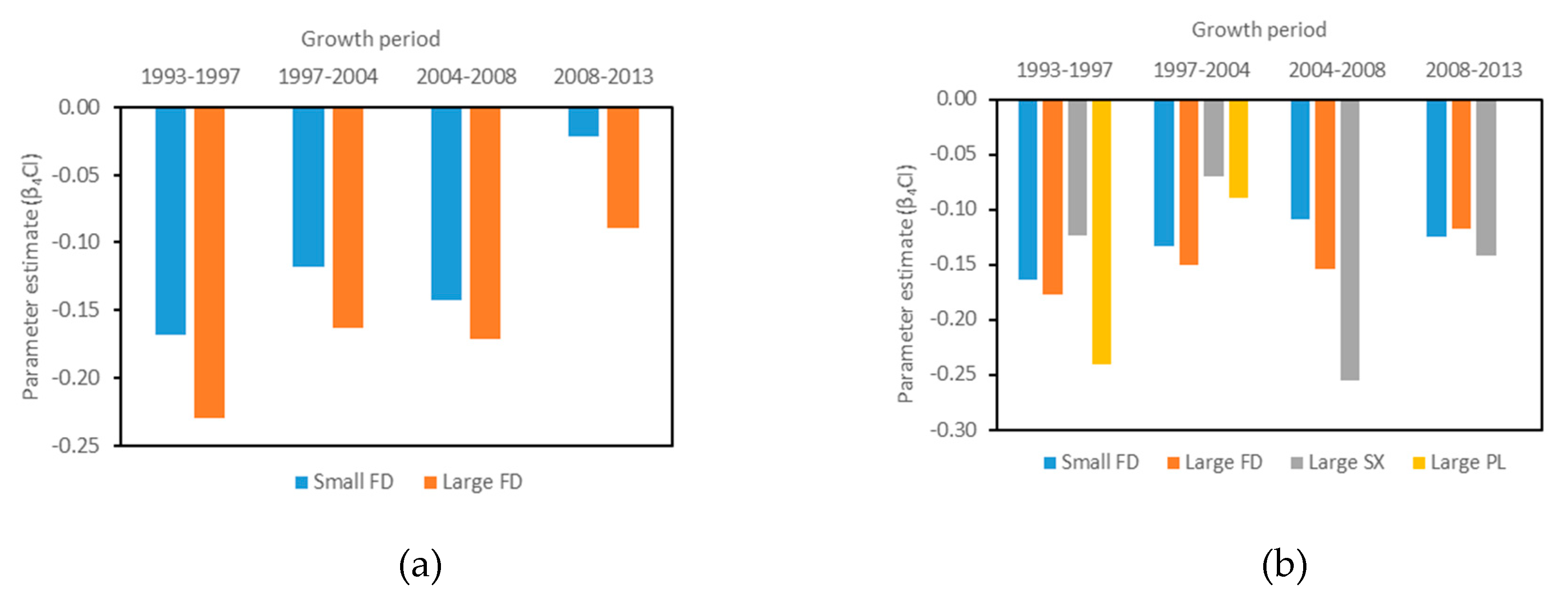
3.3. Effect of Competition on the Growth of the Subject Trees

In general, FD was projected to have higher PABAI than PL and SX for all growth periods and, not surprisingly, the growth rate declined with increasing competition levels for the three species (Figure 4a–d). Comparing the potential BA (i.e., the predicted basal area when a tree is free from competition—Figure 4a) to when a tree of a similar size is experiencing high competition (90th percentile of the competition index—Figure 4d), the loss in BA increased over time. For example, for a tree of a 20 cm DBH in 1993 in Block D, the decline in potential basal area with increasing levels of competition ranged from 10% to 39% for FD and 6% to 34% for SX over the four growth periods. The BA for PL declined by 11–15% over the first and second growth periods. Large FD were predicted to grow slightly better in Block C compared to Block D at lower levels of competition; however, the growth of FD in Block D declined less than that in Block C at higher levels of competition, resulting in similar or slightly better growth in Block D (Figure 5a–d). Similarly, small FD of a 5 or 8 cm DBH in 1993 grew slightly faster in Block C than Block D at low levels of competition, but the predicted growth was quite similar between the blocks for higher levels of competition (Figure 6a,d). FD that were 2 cm in 1993 were predicted to grow similarly in both blocks at all levels of competition.

4. Discussion

There is a finite amount of total growing space (considered as the sum total of light, moisture, and nutrients) available on a site to support trees. If there are a sufficient number of trees to occupy that growing space, then trees compete for those resources [4]. If competitive reduction exists among tree species in a mixed-species stand, it suggests that there would be differences among species in terms of their competitive impact on each other’s growth. In other words, one might expect the growth of a tree of a given species to be impacted more intensively by trees of the same species than those of other species, all other factors being equal. On the other hand, if a species’ growth is impacted more strongly by competition from trees of other species than of the same species, it would suggest that a process of competitive exclusion is taking place. It is quite possible that both processes are taking place within naturally established mixed-species stands, such as the stands we examined in this study.

We investigated whether neighboring trees compete with a subject tree independently of species identity and examined the differences in basal area growth among FD, SX, and PL over time under different degrees of competition. The Martin and Ek [30] competition index, found to be suitable for this study, is characterized by an asymmetrical relationship in which competitors share limited resources disproportionately in relation to their relative sizes [50]. This index is thought to reflect aboveground competition for light in which larger competitors pre-empt resources, making them unavailable to smaller individuals. Although multiple types of interactions can occur simultaneously in mixtures, our study found asymmetric competition to be more relevant than symmetric competition, suggesting that the main driver limiting growth in these stands is aboveground competition for light. This is not surprising as the DEC species and PL are intolerant of shade, and considered pioneer species [51], and SX and FD are considered to be moderately shade-tolerant [51,52]. This agrees with previous studies that highlight the importance of light when comparing size-asymmetric and size-symmetric competition in mixed-species stands [45,53,54].

Interactions with neighbors exerted a negative influence on basal area growth for all the subject trees we considered and these influences varied across time. These fluctuations in the intensity of competition on basal area growth over time show that temporal dynamics in resource availability, likely caused by year-to-year variations in weather (particularly precipitation patterns) and mortality of many of the larger PL, influenced the magnitude of interactions between species. Although other interactions such as facilitation and competitive reduction among species have been observed in mixed-species forests by other studies [15,55], this was not found in our study, except for small FD in Block C and large FD in Block D. In these instances, the model with the competition index partitioned by species (Equation (9)) fit best. Block C is slightly drier than Block D, and it is possible that the smaller FD is better able to compete for moisture with the other species groups than it is able to do so with itself. We did not see this phenomenon for small FD on Block D, and in fact, the model with a single competition index (Equation (8)) generally fitted best for the subject trees on that block. Further, the competition indices coefficients for the various Equation (9) fits in Block D indicated that species other than FD were exerting the most influence on the basal area growth of all the subject tree species groups. This might indicate that in the moister conditions found at Block D, species other than FD are better able to exploit belowground resources. This is consistent with this block location being considered transitional from the IDF BEC zone to the SBS BEC zone, where SX is considered to be the climax species.

The mixed results we found with respect to the impact of species identity on predicting basal area growth are consistent with what has been shown across other studies. Some studies have demonstrated differences in the species identity of neighbors in some species and the functional equivalence of neighbors in others (e.g., [56,57,58]). The apparent equivalence of neighbors in mixed-species stands has been attributed to a small sample size, which made it difficult for models to detect interspecific differences in competitive effects [20,57,58]. However, in our study, we had sufficient numbers of trees both as subject trees and as competitors. Instead, our results may be due to the complex processes occurring in multi-aged mixed-species forests where relationships between competition and tree growth may be diverse, with different species and tree sizes varying in their competitive interactions with neighboring species. In addition, the complexity of the competition environment at our sites could be compounded by variability in stochastic disturbance events or partial harvesting, which resulted in clusters of regeneration following disturbance. For example, LeMay et al. [59], in similar, but non-harvested, stands to those we examined in this study, and Druckenbrod et al. [60], found the clustering of trees at shorter distances.

The differentiation of intraspecific and interspecific competition provides useful information for understanding factors influencing tree growth and interactions between species [61]. In our study, for small FD in Block C, where a better fit was obtained when the competition index was partitioned into species or species groups, there were differences in species-specific effects. FD had, on average, stronger competitive impacts from intraspecific neighbors than from other species. Similarly, large FD in Block C and PL in Block D had stronger competition from intraspecific neighbors. Many other studies of mixed-species stands have found that intraspecific neighbors are stronger competitors than interspecific neighbors [15,45,62]. However, this effect can be positive or negative, depending on the species characteristics and site conditions, such as shade tolerance [63], stand density, and stand development [64].

We observed a higher PABAI for FD than for PL and SX, irrespective of the competition intensity. Similar growth patterns have been reported on naturally regenerated saplings of PL and FD along a wide range of light conditions, where PL showed a greater reduction in lateral growth than FD with a decreasing light availability [51]. Eis et al. [65] found that SX grows slowly, even if it started growing at the same time as PL. We expected small and large FD in Block C to grow better than small and large FD in Block D; however, at a high competition intensity, FD trees in Block D were growing at the same rate or slightly better than FD trees in Block C. This may be due to the nature of the interspecific competition experienced by FD trees in Block D versus the primarily intraspecific competition in Block C. Also, Block D is moister than Block C and belowground competition for moisture may be more limiting to growth at higher competition levels in Block C.

5. Conclusions

There was little differentiation between intraspecific and interspecific competition for the large subject trees we observed, which is consistent with competition for light in situations where the two primary species (FD and SX) are similar in shade tolerance (mid-tolerant). PL is shade-intolerant, but it grew either in less dense pockets in the stands or was one of the taller trees. Again, the species of its competitors appeared to have little impact on its basal area growth. In contrast, smaller FD were affected more heavily by intraspecific competition, suggesting that belowground competition with other FD, likely for moisture, could be playing a role, along with competition for light, in their growth. We did not have sufficient numbers of small SX trees to fit stable basal area growth prediction equations for that stand component, so we were not able to determine whether the basal area growth of these trees was also more heavily affected by competition with FD. Our models suggested that FD basal area growth, for a given tree size (DBH), was higher than that of PL and SX, irrespective of the competition level and block.

It is clear that competition is a complex process in mixed-species mixed-sized natural stands and is undoubtedly affected by a number of factors, including tree sizes, species composition, and developmental history. The relationships between periodic basal area growth and competition varied with species identity over time, likely as a result of both variations in weather (that affects moisture availability during the growing season) and disturbances. Our results provide an understanding of how IDF stands will develop over time and information on species interactions that could help forest managers design more effective silvicultural prescriptions.

References

1. Gamfeldt, L.; Snäll, T.; Bagchi, R.; Jonsson, M.; Gustafsson, L.; Kjellander, P.; Ruiz-Jaen, M.C.; Fröberg, M.; Stendahl, J.; Philipson, C.D. Higher levels of multiple ecosystem services are found in forests with more tree species. Nat. Commun. 2013, 4, 1340. [Google Scholar] [CrossRef] [PubMed]
2. Forrester, D.I.; Bauhus, J. A review of processes behind diversity—Productivity relationships in forests. Curr. For. Reports 2016, 2, 45–61. [Google Scholar] [CrossRef] [Green Version]
3. Heym, M.; Bielak, K.; Wellhausen, K.; Uhl, E.; Biber, P.; Perkins, D.; Steckel, M.; Thurm, E.A.; Rais, A.; Pretzsch, H. A new method to reconstruct recent tree and stand attributes of temporary research plots: New opportunity to analyse mixed forest stands. In Conifers; IntechOpen: London, UK, 2018; p. 44. [Google Scholar] [CrossRef] [Green Version]
4. Oliver, C.D.; Larson, B.C. Forest Stand Dynamics: Update Edition; FES Other Publications; Yale University: New Haven, CT, USA, 1996; pp. 9–39. [Google Scholar]
5. Mina, M.; del Río, M.; Huber, M.O.; Thürig, E.; Rohner, B. The symmetry of competitive interactions in mixed Norway spruce, silver fir and European beech forests. J. Veg. Sci. 2018, 29, 775–787. [Google Scholar] [CrossRef]
6. Callaway, R.M. Positive Interactions and Interdependence in Plant Communities; Springer: Dordrecht, The Netherlands, 2007; pp. 179–254. [Google Scholar]
7. Bertness, M.D.; Callaway, R.M. Positive interactions in communities. Trends. Ecol. Evol. 1994, 9, 191–193. [Google Scholar] [CrossRef]
8. Zhao, D.; Borders, B.; Wilson, M.; Rathbun, S.L. Modeling neighborhood effects on the growth and survival of individual trees in a natural temperate species-rich forest. Ecol. Model. 2006, 196, 90–102. [Google Scholar] [CrossRef]
9. Hui, G.; Wang, Y.; Zhang, G.; Zhao, Z.; Bai, C.; Liu, W. A novel approach for assessing the neighborhood competition in two different aged forests. For. Ecol. Manag. 2018, 422, 49–58. [Google Scholar] [CrossRef]
10. Burton, P.J. Some limitations inherent to static indices of plant competition. Can. J. For. Res. 1993, 23, 2141–2152. [Google Scholar] [CrossRef]
11. Li, Q.; Liang, Y.; Tong, B.; Du, X.; Ma, K. Compensatory effects between Pinus massoniana and broadleaved tree species. J. Plant Ecol. 2010, 3, 183–189. [Google Scholar] [CrossRef]
12. Hubbell, S.P.; Ahumada, J.A.; Condit, R.; Foster, R.B. Local neighborhood effects on long-term survival of individual trees in a neotropical forest. Ecol. Res. 2001, 16, 859–875. [Google Scholar] [CrossRef]
13. von Oheimb, G.; Lang, A.C.; Bruelheide, H.; Forrester, D.I.; Wäsche, I.; Yu, M.; Härdtle, W. Individual-tree radial growth in a subtropical broad-leaved forest: The role of local neighbourhood competition. For. Ecol. Manag. 2011, 261, 499–507. [Google Scholar] [CrossRef]
14. Stoll, P.; Newbery, D.M. Evidence of species-specific neighborhood effects in the Dipterocarpaceae of a Bornean rain forest. Ecology 2005, 86, 3048–3062. [Google Scholar] [CrossRef] [Green Version]
15. Pretzsch, H.; Schütze, G. Transgressive overyielding in mixed compared with pure stands of Norway spruce and European beech in Central Europe: Evidence on stand level and explanation on individual tree level. Eur. J. For. Res. 2009, 128, 183–204. [Google Scholar] [CrossRef]
16. Schwinning, S.; Weiner, J. Mechanisms determining the degree of size asymmetry in competition among plants. Oecologia 1998, 113, 447–455. [Google Scholar] [CrossRef] [PubMed]
17. Binkley, D. A hypothesis about the interaction of tree dominance and stand production through stand development. For. Ecol. Manag. 2004, 190, 265–271. [Google Scholar] [CrossRef]
18. Weiner, J.; Thomas, S.C. Size variability and competition in plant monocultures. Oikos 1986, 47, 211–222. [Google Scholar] [CrossRef] [Green Version]
19. Dale, V.H.; Doyle, T.W.; Shugart, H.H. A comparison of tree growth models. Ecol. Model. 1985, 29, 145–169. [Google Scholar] [CrossRef]
20. Uriarte, M.; Condit, R.; Canham, C.D.; Hubbell, S.P. A spatially explicit model of sapling growth in a tropical forest: Does the identity of neighbours matter? J. Ecol. 2004, 92, 348–360. [Google Scholar] [CrossRef]
21. Marshall, P.L. Response of uneven-aged Douglas-fir to alternative spacing regimes: Description of the project and analysis of the initial impact of the spacing regimes. Canada-British Columbia Economic and Regional Development Agreement. FRDA Report 242. 1996. Available online: http://203.187.160.132:9011/www.llbc.leg.bc.ca/c3pr90ntc0td/public/pubdocs/bcdocs2012_2/243652/frr242.pdf (accessed on 1 February 2020).
22. Vyse, A.; Hollstedt, C.; Huggard, D.J. Managing the Dry Douglas-Fir Forests of the Southern Interior: Workshop Proceedings: April 29–30, 1997, Kamloops, British Columbia, Canada; Vyse, A., Hollstedt, C., Huggard, D.J., Eds.; Citeseer: Kamloops, BC, Canada, 1998. [Google Scholar]
23. Hope, G.D.; Mitchell, W.R.; Lloyd, D.A.; Erickson, W.R.; Harper, W.L.; Wilkeem, B.M. Interior Douglas-Fir Zone. Ecosystems of British Columbia; Meidinger, D., Pojar, J., Eds.; Research Branch: Victoria, BC, USA, 1991; pp. 153–166. [Google Scholar]
24. Day, K. Interior Douglas-fir and selection management at the UBC/Alex Fraser Research Forest. In Proceedings of the IUFRO Uneven-Aged Silviculture Symposium, Corvallis, OR, USA, 15–19 September 1997; pp. 542–552. [Google Scholar]
25. Day, K. UBC Alex Fraser Research Forest Management and Working Plan# 3; UBC Alex Fraser Research Forest: Williams Lake, BC, Canada, 2007; 156p, Available online: https://afrf-forestry.sites.olt.ubc.ca/files/2012/03/MWP3WebQuality.pdf (accessed on 1 February 2020).
26. Marshall, P.L.; Wang, Y. Growth of Uneven-Aged Interior Douglas-Fir stands as Influenced by Different Stand Structures; Canada-British Columbia Economic and Regional Development Agreement. FRDA Report 267; Canadian Forest Service; B.C. Ministry of Forests: Victoria, BC, Canada, 1996; 20p. Available online: https://www.for.gov.bc.ca/hfd/pubs/Docs/Frr/FRR267.pdf (accessed on 1 February 2020).
27. Rivas, J.J.C.; González, J.G.Á.; Aguirre, O.; Hernández, F.J. The effect of competition on individual tree basal area growth in mature stands of Pinus cooperi Blanco in Durango (Mexico). Eur. J. For. Res. 2005, 124, 133–142. [Google Scholar] [CrossRef]
28. Kahriman, A.; Şahin, A.; Sönmez, T.; Yavuz, M. A novel approach to selecting a competition index: The effect of competition on individual-tree diameter growth of Calabrian pine. Can. J. For. Res. 2018, 48, 1217–1226. [Google Scholar] [CrossRef]
29. Contreras, M.A.M.A.; Affleck, D.; Chung, W. Evaluating tree competition indices as predictors of basal area increment in western Montana forests. For. Ecol. Manag. 2011, 262, 1939–1949. [Google Scholar] [CrossRef]
30. Martin, G.L.; Ek, A.R. A comparison of competition measures and growth models for predicting plantation red pine diameter and height growth. For. Sci. 1984, 30, 731–743. [Google Scholar] [CrossRef]
31. Steneker, G.A.; Jarvis, J.M. A preliminary study to assess competition in a white spruce-trembling aspen stand. For. Chron. 1963, 39, 334–336. [Google Scholar] [CrossRef] [Green Version]
32. Lorimer, C.G. Tests of age-independent competition indices for individual trees in natural hardwood stands. For. Ecol. Manag. 1983, 6, 343–360. [Google Scholar] [CrossRef]
33. Glover, G.R.; Hool, J.N. A basal area ratio predictor of loblolly pine plantation mortality. For. Sci. 1979, 25, 275–282. [Google Scholar] [CrossRef]
34. Krajicek, J.E.; Brinkman, K.A.; Gingrich, S.F. Crown competition—A measure of density. For. Sci. 1961, 7, 35–42. [Google Scholar]
35. Wykoff, W.R.; Crookston, N.L.; Stage, A.R. User’s guide to the stand prognosis model; USDA Forest Service General Technical Report INT-133; United States Department of Agriculture Forest Service: Ogden, UT, USA, 1982; 112p. Available online: https://www.fs.fed.us/rm/pubs_int/int_gtr133.pdf (accessed on 1 February 2020).
36. Hegyi, F. A simulation model for managing jack-pine stands. In Proceedings of the Growth Models for Tree and Stand Simulation IUFRO S4.01–4; Fries, J., Ed.; Department of Forest Yield, Royal College of Forestry: Stockholm, Sweden, 1974; pp. 74–90. [Google Scholar]
37. Rouvinen, S.; Kuuluvainen, T. Structure and asymmetry of tree crowns in relation to local competition in a natural mature Scots pine forest. Can. J. For. Res. 1997, 27, 890–902. [Google Scholar] [CrossRef]
38. Braathe, P. Height increment of young single trees in relation to height and distance of neighbouring trees. Mitteilungen der Forstl. Bundesversuchsanstalt 1980, 130, 43–48. [Google Scholar]
39. Opie, J. Predictability of individual tree growth using various definitions of competing basal area. For. Sci. 1968, 14, 314–323. [Google Scholar] [CrossRef]
40. Bella, I. A new competition model for individual trees. For. Sci. 1971, 17, 364–372. [Google Scholar] [CrossRef]
41. Monserud, R.A.; Ek, A.R. Prediction of understory tree height growth in northern hardwood stands. For. Sci. 1977, 23, 391–400. [Google Scholar] [CrossRef]
42. Pretzsch, H. Forest Dynamics, Growth and Yield. From Measurement to Model; Springer: Berlin/Heidelberg, Germany, 2009; p. 300. ISBN 978-3-540-88306-7. [Google Scholar]
43. Schröder, J.; Soalleiro, R.R.; Alonso, G.V. An age-independent basal area increment model for maritime pine trees in northwestern Spain. For. Ecol. Manag. 2002, 157, 55–64. [Google Scholar] [CrossRef]
44. Yang, Y.; Huang, S.; Meng, S.X.; Trincado, G.; Vanderschaaf, C.L. A multilevel individual tree basal area increment model for aspen in boreal mixedwood stands. Can. J. For. Res. 2009, 39, 2203–2214. [Google Scholar] [CrossRef]
45. Del Río, M.; Condés, S.; Pretzsch, H. Analyzing size-symmetric vs. size-asymmetric and intra- vs. inter-specific competition in beech (Fagus sylvatica L.) mixed stands. For. Ecol. Manag. 2014, 325, 90–98. [Google Scholar] [CrossRef] [Green Version]
46. Pinheiro, J.C.; Bates, D.M. Mixed-Effects Models in S and S-PLUS; Chambers, J., Eddy, W., Sheather, S., Tierney, L., Eds.; Springer-Verlag: New York, NY, USA, 2000; pp. 94, 306–408. ISBN 978-1-4757-8144-1. [Google Scholar]
47. R Core Team. R: A Language And Environment For Statistical Computing; R Foundation for Statistical Computing: Vienna, Austria, 2018; Available online: https://CRAN.R-project.org/package=nlme (accessed on 1 February 2020).
48. Vonesh, E.; Chinchilli, V.M. Linear and Nonlinear Models for the Analysis of Repeated Measurements; CRC Press; Marcel Dekker: New York, NY, USA, 1997; p. 546. ISBN 1482293277. [Google Scholar]
49. Wang, Y.; LeMay, V.M.; Baker, T.G. Modelling and prediction of dominant height and site index of Eucalyptus globulus plantations using a nonlinear mixed-effects model approach. Can. J. For. Res. 2007, 37, 1390–1403. [Google Scholar] [CrossRef]
50. Weiner, J. Asymmetric competition in plant populations. Trends Ecol. Evol. 1990, 5, 360–364. [Google Scholar] [CrossRef]
51. Chen, H.Y.H.; Klinka, K.; Kayahara, G.J. Effects of light on growth, crown architecture, and specific leaf area for naturally established Pinus contorta var. latifolia and Pseudotsuga menziesii var. glauca saplings. Can. J. For. Res. 1996, 26, 1149–1157. [Google Scholar] [CrossRef]
52. Kayahara, G.J.; Chen, H.Y.H.; Klinka, K.; Coates, K.D. Relations of Terminal Growth and Specific Leaf Area to Available Light in Naturally Regenerated Seedlings of Lodgepole Pine and Interior Spruce in Central British Columbia; British Columbia Minstry of Forests Research Report 09; Ministry of Forests Research Program: Victoria, BC, Canada, 1996; 32p. Available online: https://pdfs.semanticscholar.org/6881/8c2a91e483a53a3252fe01a71a89a10cf5b3.pdf (accessed on 1 February 2020).
53. Riofrío, J.; Del Río, M.; Bravo, F. Mixing effects on growth efficiency in mixed pine forests. Forestry 2017, 90, 381–392. [Google Scholar] [CrossRef] [Green Version]
54. Lu, H.; Mohren, G.M.J.; del Río, M.; Schelhaas, M.J.; Bouwman, M.; Sterck, F.J. Species mixing effects on forest productivity: A case study at stand-, species- and tree-level in the Netherlands. Forests 2018, 9, 713. [Google Scholar] [CrossRef] [Green Version]
55. Fichtner, A.; Härdtle, W.; Bruelheide, H.; Kunz, M.; Li, Y.; von Oheimb, G. Neighbourhood interactions drive overyielding in mixed-species tree communities. Nat. Commun. 2018, 9, 1144. [Google Scholar] [CrossRef] [Green Version]
56. Thorpe, H.C.; Astrup, R.; Trowbridge, A.; Coates, K.D. Competition and tree crowns: A neighborhood analysis of three boreal tree species. For. Ecol. Manag. 2010, 259, 1586–1596. [Google Scholar] [CrossRef]
57. Canham, C.D.; Papaik, M.J.; Uriarte, M.; McWilliams, W.H.; Jenkins, J.C.; Twery, M.J. Neighborhood analysis of canopy tree competition along environmental gradients in New England forests. Ecol. Appl. 2006, 16, 540–554. [Google Scholar] [CrossRef] [Green Version]
58. Coates, K.D.; Canham, C.D.; LePage, P.T. Above- versus below-ground competitive effects and responses of a guild of temperate tree species. J. Ecol. 2009, 97, 118–130. [Google Scholar] [CrossRef]
59. LeMay, V.M.; Pommerening, A.; Marshall, P. Spatio-temporal structure of multi-storied, multi-aged interior Douglas fir (Pseudotsuga menziesii var. glauca) stands. J. Ecol. 2009, 97, 1062–1074. [Google Scholar] [CrossRef]
60. Druckenbrod, D.L.; Shugart, H.H.; Davies, I. Spatial pattern and process in forest stands within the Virginia piedmont. J. Veg. Sci. 2005, 16, 37–48. [Google Scholar] [CrossRef]
61. Manso, R.; Morneau, F.; Ningre, F.; Fortin, M. Effect of climate and intra-and inter-specific competition on diameter increment in beech and oak stands. Forestry 2015, 88, 540–551. [Google Scholar] [CrossRef]
62. Adler, P.B.; Smull, D.; Beard, K.H.; Choi, R.T.; Furniss, T.; Kulmatiski, A.; Meiners, J.M.; Tredennick, A.T.; Veblen, K.E. Competition and coexistence in plant communities: Intraspecific competition is stronger than interspecific competition. Ecol. Lett. 2018, 21, 1319–1329. [Google Scholar] [CrossRef] [Green Version]
63. Dietze, M.C.; Wolosin, M.S.; Clark, J.S. Capturing diversity and interspecific variability in allometries: A hierarchical approach. For. Ecol. Manag. 2008, 256, 1939–1948. [Google Scholar] [CrossRef]
64. Mina, M.; Huber, M.O.; Forrester, D.I.; Thürig, E.; Rohner, B. Multiple factors modulate tree growth complementarity in Central European mixed forests. J. Ecol. 2018, 106, 1106–1119. [Google Scholar] [CrossRef]
65. Eis, S.; Craigdallie, D.; Simmons, C. Growth of lodgepole pine and white spruce in the central interior of British Columbia. Can. J. For. Res. 1982, 12, 567–575. [Google Scholar] [CrossRef]
Figure 1. Location of the Knife Creek Block near Williams Lake in British Columbia, Canada.
Forests 11 00167 g001
Figure 2. Parameter estimates for the Martin and Ek [30] competition index using Equation (8) for the four growth periods: (a) small (from 2.0 to 9.9 cm DBH as of 1993) and large (≥ 10.0 cm DBH as of 1993) FD as subject trees in Block C; (b) small and large FD and large SX and PL as subject trees in Block D.
Forests 11 00167 g002
Figure 3. Predicted periodic annual basal area increment versus DBH using the fixed effects parameters of the equation with partitioned CI (Equation (9)) for: (a) small interior Douglas fir in Block C; (b) large interior Douglas-fir in Block C; (c) small interior Douglas fir in Block D; (d) large interior Douglas-fir in Block D; (e) large spruce in Block D; and (f) large PL in Block D. The red, blue, green, and black lines represent the predicted PABAI for 1993–1997, 1997–2004, 2004–2008, and 2008–2013 growth periods, respectively. The red, blue, green, and black symbols represent the measured PABAI values for the same periods.
Forests 11 00167 g003
Figure 4. BA (cm2) projections in each measurement period for interior Douglas-fir (FD), spruce (SX), and lodgepole pine (PL) starting in 1993 at a 10 cm DBH (lowest set of lines), 15 cm DBH (middle set of lines), and 20 cm DBH (highest set of lines) under (a) no competition, (b) 10th percentile of competition, (c) 50th percentile of competition, and (d) 90th percentile of competition.
Forests 11 00167 g004
Figure 5. BA (cm2) projections for interior Douglas-fir growing in Blocks C and D starting in 1993 at 10 cm DBH (lowest set of lines), 15 cm DBH (middle set of lines), and 20 cm DBH (highest set of lines) under (a) no competition, (b) 10th percentile of competition, (c) 50th percentile of competition, and (d) 90th percentile of competition.
Forests 11 00167 g005
Figure 6. BA (cm2) projections for interior Douglas-fir growing in Blocks C and D starting in 1993 at 2 cm DBH (lowest set of lines), 5 cm DBH (middle set of lines), and 8 cm DBH (highest set of lines) under (a) no competition, (b) 10th percentile of competition, (c) 50th percentile of competition, and (d) 90th percentile of competition.
Forests 11 00167 g006