Predicting Tree Height-Diameter Relationship from Relative Competition Levels Using Quantile Regression Models for Chinese Fir (Cunninghamia lanceolata) in Fujian Province, China

Abstract

The importance of the height-diameter (H-D) relationship in forest productivity is well known. The general nonlinear regression model, based on the mean regression technical, is not able to give a complete description of the H-D relationship. This study aims to evaluate the H-D relationship among relative competition levels and develop a quantile regression (QR) model to fully describe the H-D relationship. The dominance index was applied to determine the relative competition levels of trees for the Chinese fir. Based on the basic Weibull growth model, the mean regression for five relative competition levels and 11 QR models was constructed with 10-fold cross-validation. We have demonstrated that the H-D relationship for the Chinese fir strongly correlated with relative competition states, but the five curves from mean regression models did not show a notable difference between the trends of H-D relationship under different competition levels. Similar regression results were found in QR models of the specific quantiles; the average tree height of five competition levels varied between 5.78% and 17.65% (i.e., about 0.06 and 0.18 quantiles). In addition, some special curves of the H-D relationship such as the QR models of the 0.01 and 0.99 quantile showed the H-D relationship under certain conditions. These findings indicate that the QR models not only evaluated the rates of change of the H-D relationships in various competition levels, but also described their characteristics with more information, like the upper and lower boundary of the conditional distribution of responses. Although the flexible QR curves followed the distribution of the data and showed more information about the H-D relationships, the H-D curves may not intersect with each other, even when the trees reached their maximum height. Hence, the QR model requires further practice in assessing the growth trajectory of the tree’s diameter or tree height to gain better results.

1. Introduction

The relationship between diameter at breast height (DBH) and tree height (H) is an important factor in forest research and is often used to estimate forest resources and wood production [1,2,3]. In the study of forest ecology and forest management, the height-diameter (H-D) relationship is one of the most important elements in estimating the stand volume and biomass, and is used as a reliable indicator of forest growth and sustainable forest management [4,5,6]. The precise estimation of the H-D relationship is essential for giving a clear description of the stand conditions and its changes over time, and can further be employed in the estimation of stand growth and yield projection [7,8]. For example, Parresol [9] described the relationship between the height and diameter of a stem as important components in yield estimation, stand description and damage appraisal. Hence, the H-D model has been widely used as an important method for obtaining tree heights and evaluating forest productivity in even or uneven-aged forests [10,11].

Various H-D models have been developed and applied for the management of different forest types [12]. The H-D model varies between stands and species; depending on the variables used, the models were classified into two types: the locally applied model and the generalized use model [13,14]. The locally applied models commonly are only dependent on tree diameter or tree age and only applicable to the stand where the data were collected [15]. On the other hand, the generalized use models, with other stand-level variables (such as site condition, competition status, environment, and climatic factors), can be applied to a large area [2,16]. According to Meyer [17], the H-D relationship is probably the most sensitive and reliable measure indicator of site productivity under natural competition. Huang and Titus [18] described the stand quality for four major species forests based on the H-D relationship of dominant and codominant trees. Kearsley et al. [19] built several H-D models and thought those useful tools improved the accuracy of forest aboveground biomass estimation, which further proved that the H-D relationship is an important feature for evaluating the competition effect on tree growth and stand yield. However, those H-D models are often modeled by the ordinary least squares (OLS) regression technique, and this method is a mean regression that may not be reliable when random and independent observations are included into the calculation [5]. Other estimation methods such as maximum likelihood (ML) and restricted estimation maximum likelihood (REML) for mixed-effect models addressed this problem and have been applied in the study of height-diameter and crown diameter prediction models [14,20]. Although these modeling approaches are better at estimating the H-D relationship, the description for the distribution of the H-D relationship may still be weak. It is difficult to predict some extremely distributed observations without prior information supported by the mixed-effect model.

Quantile regression (QR) is a method to estimate the full conditional distribution of dependent variables or quantile functions of interest, presented by Koenker et al. in 1978 [21,22]. This method is flexible in terms of describing the different distribution of the relationship between independent and dependent variables [23]. In recent years, QR has increasingly been used to study forest inventory [24], stand density [25], diameter distribution prediction [26], diameter growth [27], tree taper [28], and the aboveground biomass of forests [29]. Up to now, QR has been used in the study of tree height prediction and stand tree height simulation, but rarely reported in the relationship between age and height or diameter and height [5,30]. Unlike the mean regression method, the QR method can describe the trend of the dependent variable at any quantile. Thus, it may able to extract more information from the data, and obtain a more comprehensive analysis of the relationship between height and diameter [31,32].

The Chinese fir (Cunninghamia lanceolata(Lamb.)Hook.) has the largest afforestation area in South China. Due to its rapid growth and excellent wood quality, this species has remarkable economic value and important ecological benefits [33,34]. To the authors’ knowledge, although there have been a large number of studies conducted based on the H-D models to estimate the relationship between height and diameter in Chinese fir plantations [35,36], few studies have considered the QR approach. In addition, only scant attention has been paid to a comprehensive analysis of the relationship between height and diameter, especially for the application to non-dominant trees [1,11,37]. Therefore, the ability of the QR models to describe and evaluate the H-D relationships of the Chinese fir has not been fully validated.

To address the aforementioned problems, the goals of this study were to: (i) quantify the five relative competition levels of the Chinese fir, (ii) develop and evaluate H-D models applying mean regression and quantile regression approaches for the five competition levels, and (iii) compare the H-D curves in different competition levels to analyze the growth relationship between DBH and H at each level.

2. Materials and Methods

2.1. Data Collection

The data used in this study were collected from the National Forest Farm at Jiangle County, northwest Sanming City, southeastern China (117°05′–117°40′ E, 26°26′–27°04′ N) in July 2018. The region experiences a subtropical monsoon climate, with an annual average temperature of 18.6 °C and annual average precipitation of 1721.6 mm. Precipitation is concentrated in the summer. Plantation species in the forest farm include Chinese fir, Pinus massoniana Lamb., Schima superba Gardn. et Champ, Michelia macclurei Dandy, and Phyllostachys heterocycla (Carr.) Mitford cv. Pubescens.

Data for this study were obtained from the even-aged and pure stands plantation (more than 85%) throughout the forest farm. A total of 3133 trees in 28 sample plots (five temporary and 23 permanent) were investigated from the study area and set up in five age groups, including young forests (1–10 years), middle-age forests (11–20 years), nearly mature forests (21–25 years), mature forests (26–35 years) and over-mature forests (≥36 years). The projected area size of plots ranged from 400 to 900 m², depending on the stand density. The plot size of dense stands is 400 and 600 m², while the plot size of sparse stands is 600 and 900 m². In each plot, we recorded its coordinates, elevation, slope aspect, degree, and position. The tree characteristics such as species, DBH (>4 cm, measured at 1.3 m above ground), H, crown width (CW), and the dominance tree height (DH) of the stand were measured (

Table 1. Summary statistics of tree and stand variables in plots considered for five distinct age groups.

Age groups	Measurement	Mean	S.D.	Min.	Max.
Young (575 trees in three plots)	DBH (cm)	8.47	2.47	4.00	18.90
	H (m)	6.34	2.23	2.30	14.40
	CW (m)	2.25	0.75	0.50	5.50
	N (trees/ha)	3255	456	2625	3689
	DH (m)	10.49	2.92	6.24	12.86
Middle-aged (866 trees in eight plots)	DBH (cm)	15.64	4.52	5.00	31.00
	H (m)	14.82	3.17	5.80	23.90
	CW (m)	3.05	1.24	0.50	9.30
	N (trees/ha)	2208	391	1367	2644
	DH (m)	19.38	1.51	17.40	23.24
Nearly mature (645 trees in six plots)	DBH (cm)	15.46	6.23	4.40	36.50
	H (m)	16.24	4.50	3.40	26.50
	CW (m)	3.29	1.55	0.20	6.90
	N (trees/ha)	2247	553	1000	3083
	DH (m)	22.48	1.55	20.56	26.18
Mature (755 trees in seven plots)	DBH (cm)	18.21	7.71	4.70	53.50
	H (m)	17.32	5.00	6.00	31.99
	CW (m)	3.59	1.68	0.40	10.20
	N (trees/ha)	1846	685	1025	3000
	DH (m)	24.29	1.15	22.74	27.66
Over-mature (292 trees in four plots)	DBH (cm)	23.77	6.87	4.00	41.10
	H (m)	21.01	4.31	4.50	27.40
	CW (m)	3.77	1.67	0.50	8.10
	N (trees/ha)	1217	395	700	1767
	DH (m)	25.99	0.43	25.54	26.62

Note: S.D., Min. and Max. is an abbreviation for standard deviation, minimum and maximum.

). The tree positions (relative x, y coordinates) were recorded by grids of subplots (10 × 10 m) and a distance measurer. The southwest corner of each plot was assigned as the origin point for tree position measurement, and the x, y coordinates were measured to the nearest 0.05 m.

In order to avoid the edge effect in the dominance index calculation, a 2-m buffer was set up along the sample plot boundaries [38]. The trees in the buffer zone were only considered in the neighborhood structure [39].

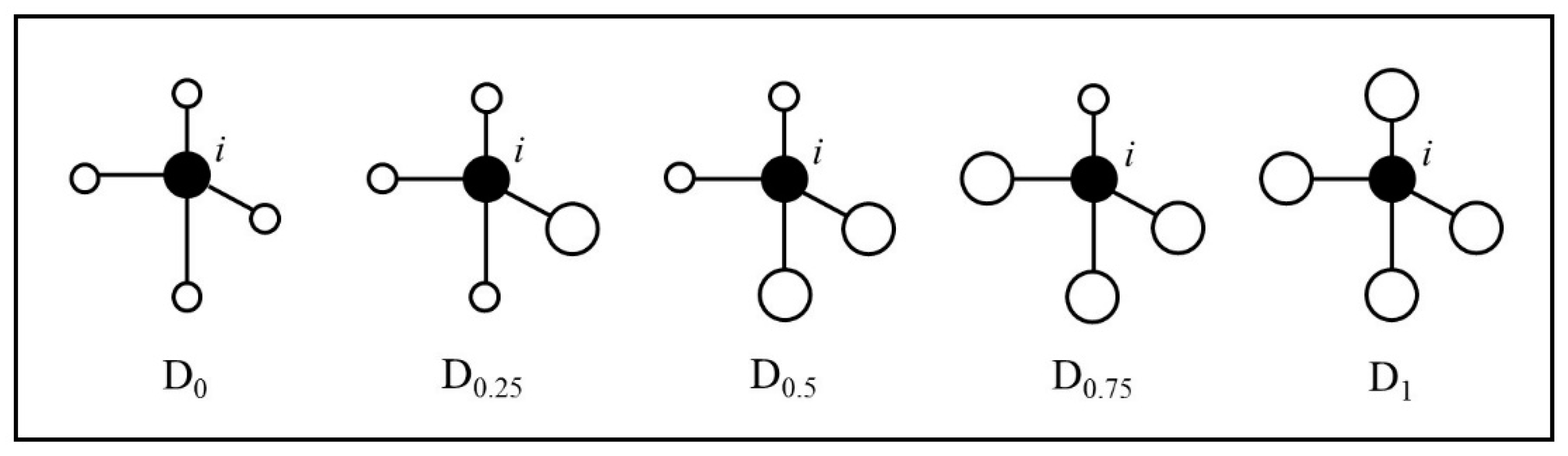
2.2. Relative Competition Quantification

Based on the neighboring trees, the Hegyi competition index and the dominance index were both used to quantifying the competition at the individual tree level [40,41]. The former has a higher accuracy of quantification, which is applied to the study of competition intensity with growth. The latter estimates the relative competition pattern, which simplifies the process of quantification and weakens the effects of abnormal trees [42]. Due to these characteristics, the dominance index is more applicable to our objective. Therefore, the trees were divided into five relative competition levels by using the dominance index (D_i). The index expresses the degree of difference in the tree’s characteristics (such as DBH, H, volume, and biomass) [43]. The dominance index is defined as the ratio of a certain number of neighboring trees that are larger than the reference tree. The equation is as follows:

$${\mathrm{D}}_i=\frac{1}{n}{{\displaystyle \sum }}_{j=1}^n{k}_{ij},$$

(1)

where $k_{ij}=\{\begin{array}{l}0,ifreferencetreeilargerthanneighboringtreej,\hfill \\ 1,otherwise.\hfill \end{array}$

In this study, difference in DBH was used to obtain the value of k_ij, and the number of neighboring trees n was set as 4. Therefore, the value of dominance included 0, 0.25, 0.5, 0.75 and 1, representing five competition levels, i.e., predominant (D₀), dominant (D_0.25), co-dominant (D_0.5), suppressed (D_0.75), and inferior (D₁) (Figure 1). A larger D_i value indicates that the reference tree is under competitive pressure [44].

The dominance indices of trees were calculated using the “forestSAS” package (version 1.0.1) [45] in R (version 3.6.0).

2.3. Base Model

Several base H-D relationship functions were selected based on previous studies [12,13,15,46]. Based on a preliminary analysis (not shown), the Weibull function fits the data best, which is similar to the findings of studies of Özçelik [5] and Yang [47]. The base function is as follows:

$$H_{ij}=1.3+\left(a+b·D{H}_i\right)·{[1-\exp (-c·DB{H}_{ij})]}^d,$$

(2)

where H_ij and DBH_i are, respectively, the total height (m) and diameter at breast height (cm) of the jth tree in the ith plot; DH_i is the dominant height of the ith plot; and a, b, c, and d are the regression parameters.

2.4. Quantile Regression Model

For a nonlinear QR model, Equation (2) was used to predict the $\mathsf{\tau }\mathrm{th}$ quantile. The quantile regression model is as follows:

$$\widehat{H_{\tau }}\left(DB{H}_{ij}\right)=1.3+\left(a+b·{\mathrm{DH}}_i\right)·{[1-\exp (-c·DB{H}_{ij})]}^d,$$

(3)

where $\widehat{H_{\tau }}\left(DB{H}_{ij}\right)$ is the predicted value of the $\mathsf{\tau }\mathrm{th}$ quantile of tree height at diameter DBH_ij. The function computes an estimate on the $\mathsf{\tau }\mathrm{th}$ conditional quantile function of the response, given the covariates, as specified by the formula argument [21,48].

Parameters from the quantile regression were obtained by minimizing the following problem [49]:

$$\min \left\{{{\displaystyle \sum }}_{H\ge \widehat{H_{\tau }}\left(DB{H}_{ij}\right)}\tau \left[H_{ij}-\widehat{H_{\tau }}\left(DB{H}_{ij}\right)\right]+{{\displaystyle \sum }}_{H\ge \widehat{H_{\tau }}\left(DB{H}_{ij}\right)}\left(1-\tau \right)\left[\widehat{H_{\tau }}\left(DB{H}_{ij}\right)-H_{ij}\right]\right\}.$$

(4)

The “quantreg” package (version 5.51) was used to develop a set of series quantile regression models; the observations and parameters belong to the moderate-sized (n $\ll$ 5000, p $\ll$ 20) category, so it is recommended that the default “br” method be used [48].

2.5. Evaluation and Testing

To compare the fit of basic H-D models, 10-fold cross-validation [50] and the following criteria for evaluation were chosen: Akaike information criterion (AIC), Bayesian Information Criterions (BIC), log-likelihood value (logLik), root mean squared error (RMSE), coefficient of determination (R²), and mean absolute error (MAE).

$$AIC=2k-2ln\left(\widehat{L}\right)$$

(5)

$$BIC=\ln \left(n\right)2k-2\ln \left(\widehat{L}\right)$$

(6)

$$RMSE= \sqrt{\frac{1}{n}{{\displaystyle \sum }}_{i=1}^n{\left(y_i-{\widehat{y}}_i\right)}^2},$$

(7)

$${\mathrm{R}}^2=1-\frac{{{\displaystyle \sum }}_{i=1}^n{\left(y_i-{\widehat{y}}_i\right)}^2}{{{\displaystyle \sum }}_{i=1}^n{\left(y_i-{\overline{y}}_i\right)}^2},$$

(8)

$$MAE=\frac{1}{n}{\displaystyle \sum }_{i=1}^n\left|y_i-{\widehat{y}}_i\right|,$$

(9)

where $\widehat{L}$ is the likelihood function for the model; y_i and ${\widehat{y}}_i$ are the observed and predicted values of tree height, respectively; and ${\overline{y}}_i$ is the average value of y_i. All calculations were performed using R (R 3.6.0 for Windows). The core code can be found in Appendix A.

3. Results

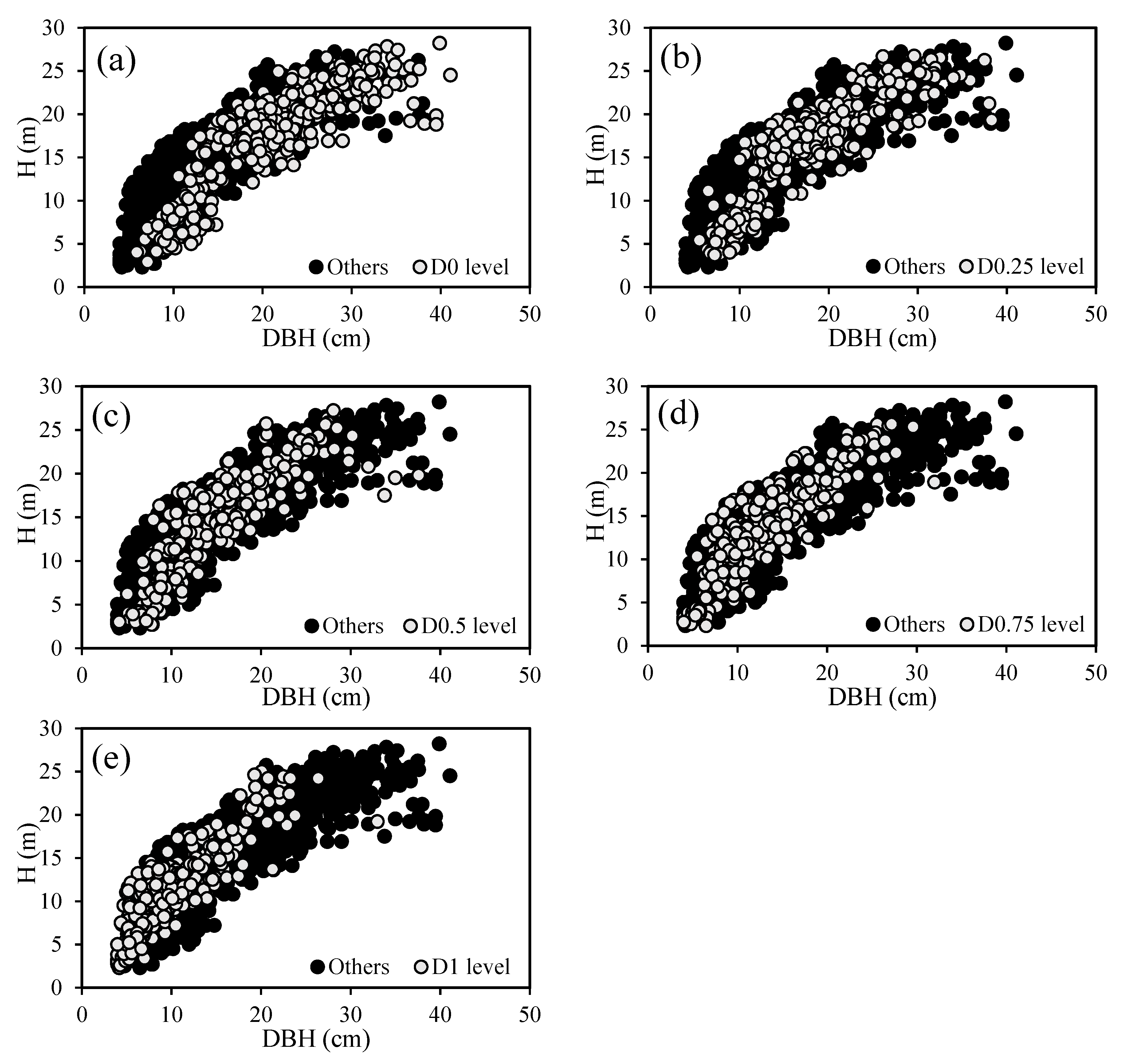
3.1. The Quantification of Five Relative Competition Levels

The statistical results (

Table 2. Summary statistics of trees for each relative competition levels without trees in buffer.

Relative Competition Levels	No. of Trees	DBH				H
		Mean	S.D.	Min.	Max.	Mean	S.D.	Min.	Max.
D0	425	20.6	7.3	5.9	41.1	17.3	5.8	2.9	28.2
D0.25	382	17.8	6.5	5.5	38.3	16.3	5.5	3.7	26.7
D0.5	352	15.0	6.0	4.2	37.6	14.7	5.7	2.7	27.2
D0.75	361	13.3	5.3	4.0	32.0	13.6	5.1	2.3	25.6
D1	350	10.2	4.8	4.0	33.0	11.2	4.9	2.3	25.0
Total	1870	15.6	7.1	4.0	41.1	14.8	5.8	2.3	28.2

S.D. is an abbreviation for standard deviation.

) showed the characteristics of DBH and H in each relative competition level, and their changes with competition levels. The difference in the DBH between the competition levels ranged from 11.33% to 23.31% with the increase in competitive pressure (D₀ to D₁ level), while the difference in tree height ranged from 5.78% to 17.65%. The proportions of trees, starting from the competition level D₀ to D₁, are 22.73%, 20.43%, 18.82%, 19.30%, and 18.72%, respectively, which shows that the number of trees at the five levels is not very different.

According to the plotting of H-D relationships for five levels (Figure 2), the distribution and trend changes of H-D for the D₀ level (Figure 2a) are relatively lower than (or to the right of) the other levels, whereas for the D_0.75 and D₁ levels (Figure 2d,e), they are relatively higher than (or to the left of) the other levels. To an extent, the clear distribution of the H-D relationships among the five competition levels proved the applicability of the dominance index in the relative competition quantification.

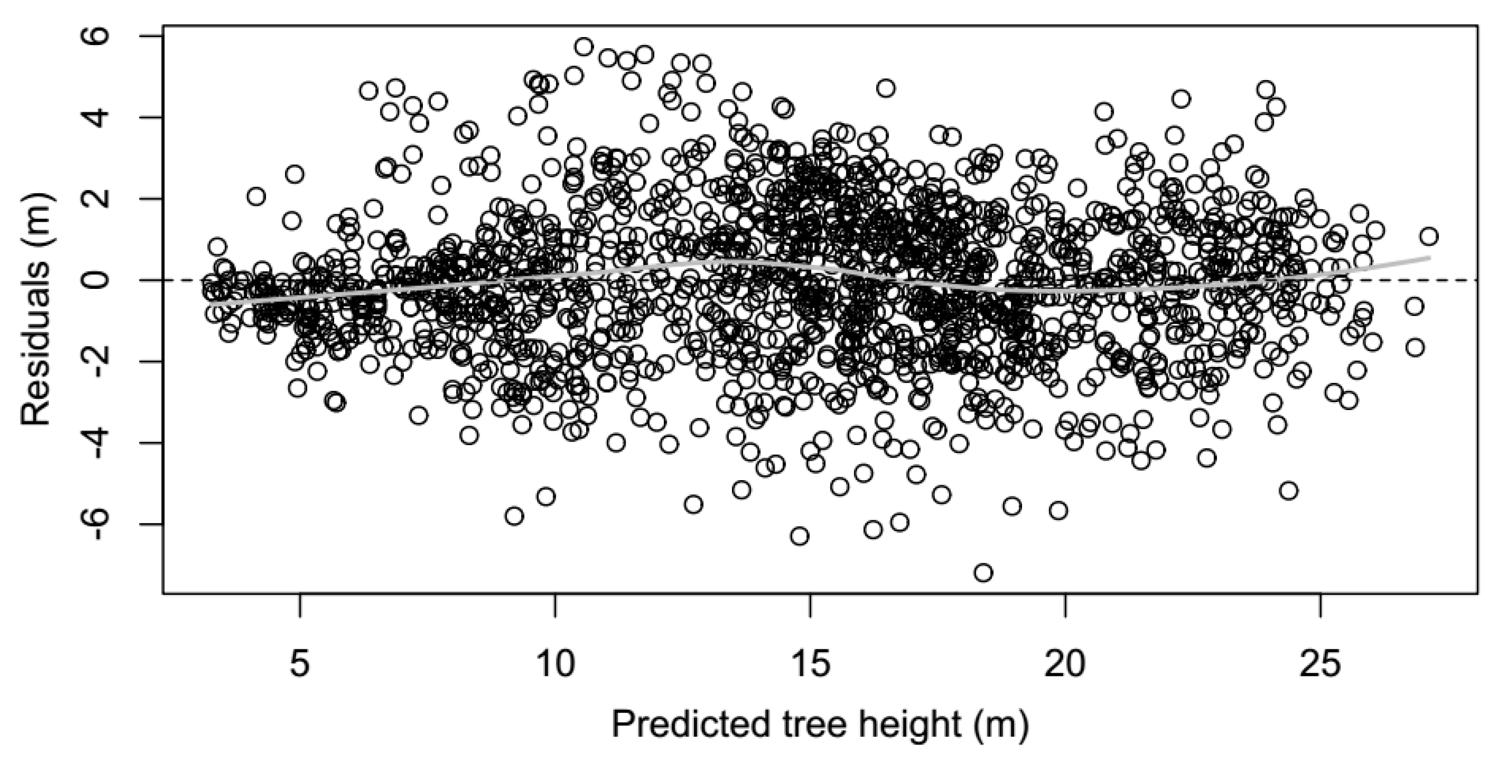
3.2. Base H-D Model Validation

The parameter estimates and fit statistics for base H-D models of the Chinese fir are listed in

Table 3. Details of 10-fold cross-validation for base models.

Fold	AIC	BIC	logLik	Training Group			Testing Group
				RMSE	MAE	R2	RMSE	MAE	R2
1	6881.5	6908.6	−3435.7	1.8636	1.449	0.901	1.8707	1.4747	0.8931
2	6888.2	6915.3	−3439.1	1.865	1.4545	0.9003	1.8555	1.4217	0.8999
3	6926.6	6953.8	−3458.3	1.8864	1.4703	0.8982	1.6479	1.296	0.9193
4	6863.7	6890.8	−3426.8	1.856	1.4494	0.9006	1.9349	1.4941	0.8974
5	6895.0	6922.1	−3442.5	1.8734	1.4595	0.8993	1.7779	1.389	0.9087
6	6833.8	6861.0	−3411.9	1.8374	1.4357	0.9027	2.0886	1.6167	0.8791
7	6885.5	6912.6	−3437.7	1.8658	1.4475	0.8997	1.8493	1.5116	0.9053
8	6869.7	6896.9	−3429.9	1.8571	1.4459	0.9014	1.9263	1.5266	0.8898
9	6853.3	6880.4	−3421.6	1.848	1.4419	0.9014	2.0025	1.5416	0.8908
10	6919.8	6946.9	−3454.9	1.8849	1.4723	0.8983	1.6660	1.2747	0.9180

Note: The coefficients (a, b, c and d) of models (not shown) are all significant (p-value < 0.001).

. All of the models that produced the H-D relationship performed well, with R² ranging from 0.8982 to 0.9027 in the training group, and with low RMSE and MAE ranging from 1.6479 to 2.0886 and 1.2747 to 1.6167, respectively, in the testing group. The fold-6th model had the lowest values of AIC, BIC, and the largest values of logLik; R² predicted the best results for training data. The coefficients of this model are a (5.6653), b (0.7755), c (0.0832), and d (1.3265). Hence, this model was further tested, and the residual plot (Figure 3) shows homoscedasticity, which confirms that other weights were unnecessary. Therefore, the base model is suitable for H-D relationship fitting.

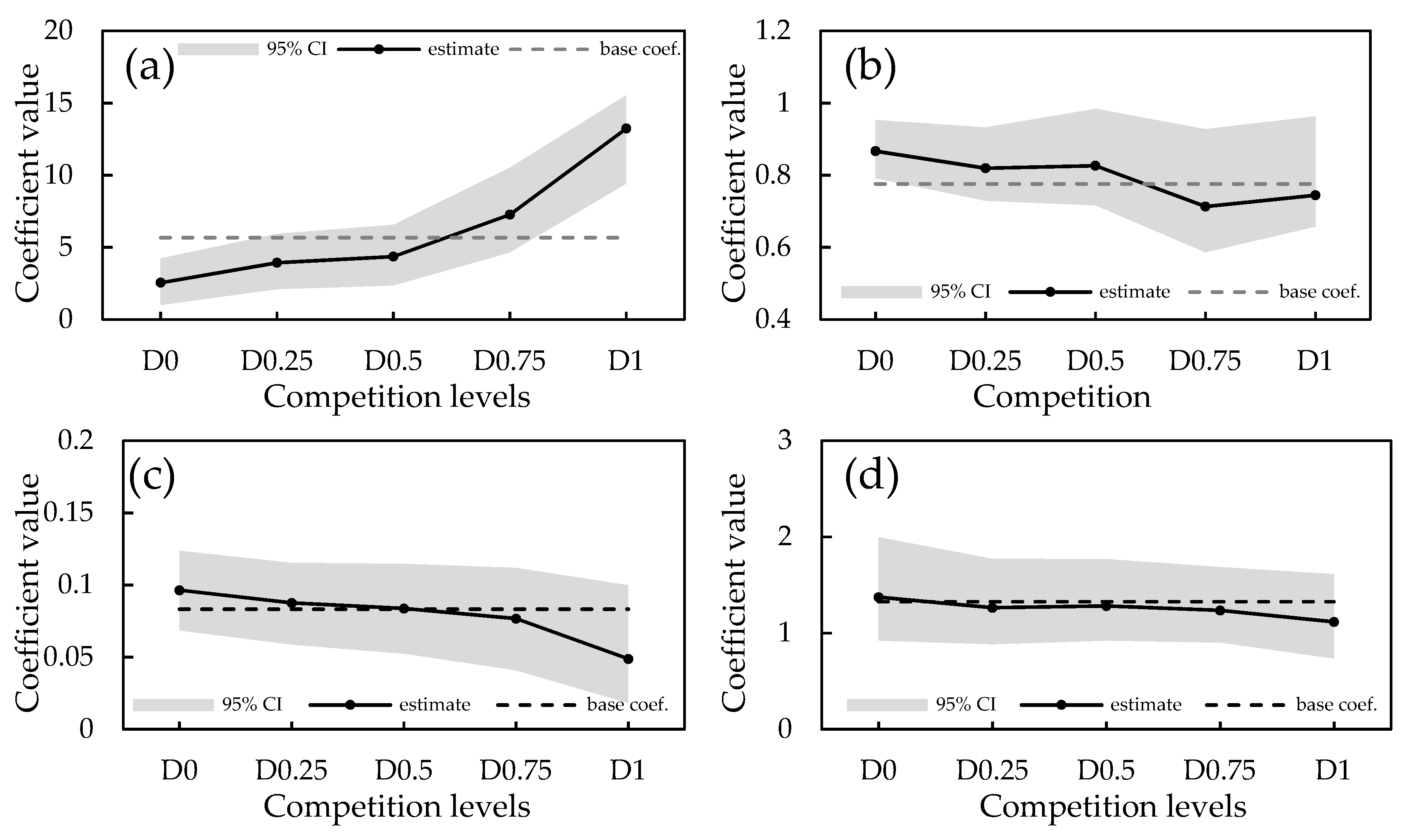
3.3. Mean Regression Models for Five Competition Levels

The parameters and summary statistics of H-D models for five competition levels are listed in

Table 4. The summary statistics of optimal H-D models for five competition levels from 10-fold cross-validation.

	D0	D0.25	D0.5	D0.75	D1
AIC	1463.3	1338.3	1271.8	1364.1	1326.2
BIC	1483.1	1357.5	1290.6	1383.0	1344.9
logLik	−726.7	−664.2	−630.9	−677.1	−658.1
RMSE (Training)	1.6135	1.6683	1.7817	1.9432	1.9677
MAE (Training)	1.2978	1.3250	1.3699	1.5277	1.5641
R2 (Training)	0.9256	0.9086	0.9069	0.8537	0.8440
RMSE (Testing)	2.0513	1.9273	2.3651	2.2568	2.4648
MAE (Testing)	1.5157	1.5042	1.8294	1.7752	1.8375
R2 (Testing)	0.8724	0.8844	0.7998	0.8334	0.7431

Note: Training and Testing in brackets indicate the training group and testing group of data for modeling and validation.

, and the different model coefficients with 95% confidence interval (CI) between the five competition levels are shown in Figure 4. Depending on the coefficient change trend of the models between each level, the difference among the competition levels could be observed by the change ratio of the coefficients. In the Weibull model we used, the coefficients before the natural logarithm “e” (including a and b) are directly proportional to the ratio of H-D and the maximum tree height. The coefficients c and d related to the rate at which the tree height reaches the maximum tree height with increasing DBH. For example, the model coefficients c and d of the D₁ are 36.46% and 9.69% smaller than D_0.75. Therefore, the difference of H-D relationship trend between each competition level can be judged by the rate of change of the model’s coefficients. However, the rates of change for the H-D relationships near the upper boundary of the conditional distribution of H-D relationships are still unclear [31], which shows that the conventional mean regression may be inappropriate or limited for estimating the H-D relationships with ungraded data for competition level.

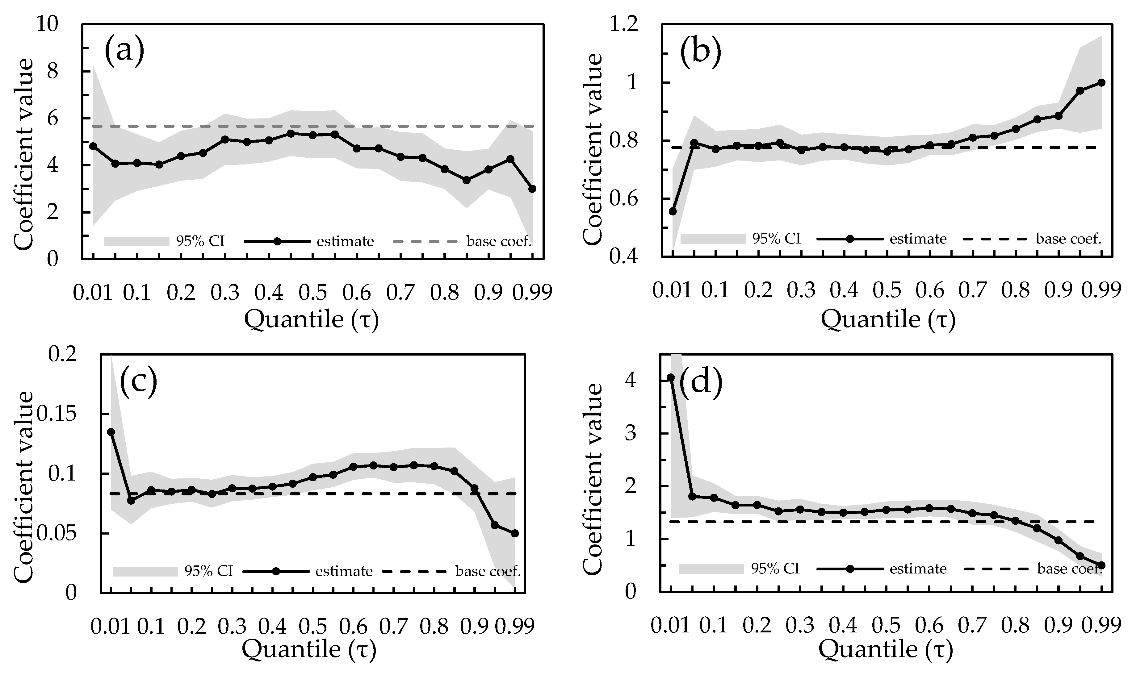
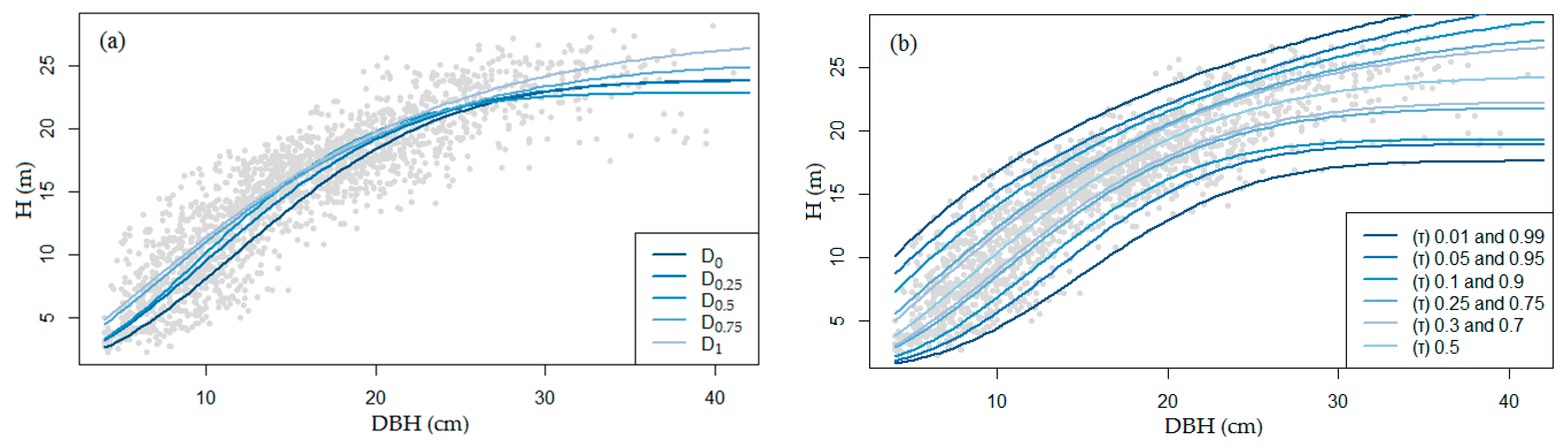
3.4. Quantile Regression Models

According to the results of the quantile process for all trees (Figure 5), the variation trends of the QR models in some specific quantiles were similar to the other competition model’s parameters (a, b, c and d). This means that the QR model may be used to predict the H-D relationship of trees at different competition levels. The median quantile (τ = 0.5) model and multiple quantiles like τ = 0.4 and τ = 0.6 were similar to the basic model, while other quantiles were also informative. The prediction of the QR model for τ = 0.01 and τ = 0.99 may indicate the upper and lower boundary of the conditional distribution of the H-D relationship. Trees in the 0.01 and 0.99 quantile have only 1% of trees showing their respective H-D relationship trend, so may commonly be considered as outliers or prediction errors in the modeling process.

3.5. Comparison of Modeling Approaches

In order to illustrate the behavior of the H-D model and to compare the application capabilities of the two methods in practice, the H-D curves (as a stand height curve) fitted by the two methods were plotted (Figure 6). The comparison results showed that the H-D relationships of the five different competition levels fitted by the mean regression (Figure 6a) might not be clearly distinguished. On the other hand, the quantile regression fitted the H-D curves of different shapes based on the different distribution characteristics of tree height increasing with DBH, which is flexible and more informative about the H-D relationships (e.g., combined with the H-D relationship distributions of the five competition levels, the dominant trees (D₀) were mostly distributed in the 0.01 to 0.25 quantile range; the medium trees (D_0.5) were mainly distributed in the 0.25 to 0.75 quantile range; the suppressed woods (D₁) were mostly distributed in the 0.75 to 0.99 quantile range). However, the limitations of quantile regression are also obvious: the fitted curve of the model follows the distribution of the observed data and the basic shapes dictated by the quantile regressions [5], thus preventing the curves from crossing one another (when the tree reached its maximum height; the maximum height of the Chinese firs in this study area is about 24 m).

4. Discussion

To clarify the relationship between the height and diameter in different competition conditions, the mean regression and QR models for the H-D relationship were developed based on the Weibull growth model, and compared in this study. With the same coefficients of the H-D models, the estimation of the QR covered most of the predicted observations from the five competition level mean regression models. To compare the variation of the model parameters, the parameters in the five competitive mean regression models were consistent with the parameters in the QR model on the quantile between 0.3 and 0.7, which shows that the average tree height of five competition levels varied between 5.78% and 17.65% (i.e., about 0.06 and 0.18 quantiles). This shows that it is feasible to predict the H-D relationship curves of different competition levels or describe the various types of growth patterns with specific quantile regression models [51,52]. In addition, we can deduce the current growth and competition of trees by referring to the conditional distribution of the H-D relationship in the QR model. If the tree does not reach the maximum tree height, the current H-D relationship can be used to estimate its respective competition level. The H-D relationship of the dominant tree is closer to the lower boundary of the H-D distribution [31], i.e., the low quantile (0.01–0.3), while the suppressed tree is closer to the upper boundary of the H-D distribution, i.e., the high quantile (0.7–0.99). This rule is consistent with the general situation of tree growth [27,37], while the mean regression model cannot effectively quantify this phenomenon under this distribution range [30].

For most H-D growth relationship research in the forestry and ecology fields, the conditional mean of dependent variables is most important for statistical modeling, but sometimes researchers are more interested in the outliers or extreme values of the dependent variable. The quantile regression results in the median quantile range are similar to the mean regression results [31,53], and this is also confirmed by the fitting results of model parameters in this study. However, based on the characteristics of the QR model, the conditional distribution of the dependent variable is fully described by quantile regression and is therefore of more interest to researchers. The curves of the QR model are often used to explore the abnormal growth in the study of growth charts [54,55]. On the one hand, the QR model provides a more detailed view of the growth trend (e.g., the H-D relationship in this study) of trees in describing the structural distribution and changes to the H-D relationship. On the other hand, the QR models predict the H-D relationship assuming that the predictor variables have a specific distribution in response to different conditions, in this case, the competition levels [31].

Although the QR model is reliable in some studies, there are two problems that have to be solved for its practical application. First, when the distribution of the dependent variable (i.e., tree height) is concentrated in the data, there was no significant difference between the QR models. The QR models in this study showed concentrated distribution of dependent variable from 0.4 to 0.6 quantiles, similar to the previous study of the tree height prediction [27]; as a result, these QR models did not differ significantly. However, when the standard deviation of the tree height was large, or the dispersion degree of the H-D relationship was obvious, as in this study, the QR models of different quantiles were significantly different. Therefore, for the QR model, the distribution of the data may be as important as the quantile selection. Second, the growth trends of trees in fact crossed each other, while the growth trend curves fitted by QR are not allowed to do so as the QR curves usually follow the distribution of the data and the guidance of the base shape [22,48]. Therefore, the QR model may be more suitable for research about classification by models (such as the site index model and growth dynamics model). In conclusion, the distribution of data and the base guiding curve are the main issues that should be considered for QR model fitting.

5. Conclusions

An accurate and complete description of the H-D relationship is key to forest monitoring and decision-making for sustaining and improving the understanding of ecological functions in plantation systems. In our study, the five relative competition levels of the Chinese fir were quantified by the dominance index. The difference in the DBH between the competition levels ranged from 11.33% to 23.31% with the increase in competitive pressure (D₀ to D₁ level), and the tree height ranged from 5.78% to 17.65%. To describe the various H-D relationship, the mean regression and the QR models of the H-D relationship were compared. The H-D relationships between each competition level were not markedly different for the fitted curves of mean regression. However, the regression curves based on different quantiles showed various trends that can clearly describe the H-D relationship among these competition levels. The average tree height between the five competition levels varied between 0.06 and 0.18 quantiles. The flexible and informative QR models showed some special curves of the H-D relationship in the 0.01 and 0.99 quantile, which might cover the particular H-D relationships under extreme conditions. However, the limitation of the QR models is obvious: the fitted curves are unable to cross one another because the curve of the model follows the distribution of observed data and the basic shapes dictated by the quantile regressions. Hence, the QR model requires further improvement in assessing the growth trajectory of the tree’s diameter or height to gain better results.

References

1. Fu, L.; Lei, X.; Sharma, R.P.; Li, H.; Zhu, G.; Hong, L.; You, L.; Duan, G.; Guo, H.; Lei, Y.; et al. Comparing height–age and height–diameter modelling approaches for estimating site productivity of natural uneven-aged forests. For. Int. J. For. Res. 2018, 91, 419–433. [Google Scholar] [CrossRef]
2. Trorey, L.G. A Mathematical Method for the Construction of Diameter Height Curves Based on Site. For. Chron. 1932, 8, 121–132. [Google Scholar] [CrossRef]
3. Stout, B.B.; Shumway, D.L. Site Quality Estimation Using Height and Diameter. Forest Sci. 1982, 28, 639–645. [Google Scholar]
4. Crecente-Campo, F.; Tomé, M.; Soares, P.; Diéguez-Aranda, U. A generalized nonlinear mixed-effects height–diameter model for Eucalyptus globulus L. in northwestern Spain. For. Ecol. Manag. 2010, 259, 943–952. [Google Scholar] [CrossRef] [Green Version]
5. Özçelik, R.; Cao, Q.V.; Trincado, G.; Göçer, N. Predicting tree height from tree diameter and dominant height using mixed-effects and quantile regression models for two species in Turkey. Forest Ecol. Manag. 2018, 419–420, 240–248. [Google Scholar] [CrossRef]
6. Kang, H.; Seely, B.; Wang, G.; Cai, Y.; Innes, J.; Zheng, D.; Chen, P.; Wang, T. Simulating the impact of climate change on the growth of Chinese fir plantations in Fujian province, China. Nz. J. For. Sci. 2017, 47, 20. [Google Scholar] [CrossRef]
7. Huang, S.; Wiens, D.P.; Yang, Y.; Meng, S.X.; Vanderschaaf, C.L. Assessing the impacts of species composition, top height and density on individual tree height prediction of quaking aspen in boreal mixedwoods. Forest Ecol. Manag. 2009, 258, 1235–1247. [Google Scholar] [CrossRef]
8. Arney, J.D. A modeling strategy for the growth projection of managed stands. Can. J. Forest Res. 1985, 15, 511–518. [Google Scholar] [CrossRef]
9. Parresol, B.R. Baldcypress height–diameter equations and their prediction confidence intervals. Can. J. Forest Res. 1992, 22, 1429–1434. [Google Scholar] [CrossRef]
10. Larsen, D.R.; Hann, D.W. Height-Diameter Equations for Seventeen Tree Species in Southwest Oregon; Oregon State University, College of Forestry, Forest Research Laboratory: Corvallis, OR, USA, 1987; Volume 49. [Google Scholar]
11. Vanclay, J.K. Tree diameter, height and stocking in even-aged forests. Ann. Forest Sci. 2009, 66, 702. [Google Scholar] [CrossRef] [Green Version]
12. Huang, S.; Price, D.J.; Titus, S. Development of ecoregion-based height–diameter models for white spruce in boreal forests. Forest Ecol. Manag. 2000, 129, 125–141. [Google Scholar] [CrossRef]
13. Lei, X.; Peng, C.; Wang, H.; Zhou, X. Individual height–diameter models for young black spruce (Picea mariana) and jack pine (Pinus banksiana) plantations in New Brunswick, Canada. For. Chron. 2009, 85, 43–56. [Google Scholar] [CrossRef] [Green Version]
14. Sánchez-González, M.; Cañellas, I.; Montero, G. Generalized height-diameter and crown diameter prediction models for cork oak forests in Spain. Investig. Agrar. Sist. Recur. For. 2007, 16. [Google Scholar] [CrossRef] [Green Version]
15. Newton, P.F.; Amponsah, I.G. Comparative evaluation of five height–diameter models developed for black spruce and jack pine stand-types in terms of goodness-of-fit, lack-of-fit and predictive ability. Forest Ecol. Manag. 2007, 247, 149–166. [Google Scholar] [CrossRef]
16. Schumacher, F.X.; Day, B.B. The Influence of Precipitation upon the Width of Annual Rings of Certain Timber Trees. Ecol. Monogr. 1939, 9, 387–429. [Google Scholar] [CrossRef]
17. Meyer, H.A. A Mathematical Expression for Height Curves. J. For. 1940, 38, 415–420. [Google Scholar] [CrossRef]
18. Huang, S.; Titus, S.J. An index of site productivity for uneven-aged or mixed-species stands. Can. J. Forest Res. 1993, 23, 558–562. [Google Scholar] [CrossRef]
19. Kearsley, E.; Moonen, P.C.J.; Hufkens, K.; Doetterl, S.; Lisingo, J.; Boyemba Bosela, F.; Boeckx, P.; Beeckman, H.; Verbeeck, H. Model performance of tree height-diameter relationships in the central Congo Basin. Ann. For. Sci. 2017, 74. [Google Scholar] [CrossRef] [Green Version]
20. Paulo, J.A.; Tomé, J.; Tomé, M. Nonlinear fixed and random generalized height–diameter models for Portuguese cork oak stands. Ann. For. Sci. 2011, 68, 295–309. [Google Scholar] [CrossRef] [Green Version]
21. Koenker, R.; Bassett, G. Regression Quantiles. Econometrica 1978, 46. [Google Scholar] [CrossRef]
22. Furno, M.; Vistocco, D. Quantile Regression: Estimation and Simulation; John Wiley & Sons: Hoboken, NJ, USA, 2018. [Google Scholar]
23. Kocherginsky, M.; He, X.; Mu, Y. Practical Confidence Intervals for Regression Quantiles. J. Comput. Graph. Stat. 2005, 14, 41–55. [Google Scholar] [CrossRef]
24. Mäkinen, A.; Kangas, A.; Kalliovirta, J.; Rasinmäki, J.; Välimäki, E. Comparison of treewise and standwise forest simulators by means of quantile regression. Forest Ecol. Manag. 2008, 255, 2709–2717. [Google Scholar] [CrossRef]
25. Ducey, M.J.; Knapp, R.A. A stand density index for complex mixed species forests in the northeastern United States. Forest Ecol. Manag. 2010, 260, 1613–1622. [Google Scholar] [CrossRef]
26. Mehtätalo, L.; Gregoire, T.G.; Burkhart, H.E. Comparing strategies for modeling tree diameter percentiles from remeasured plots. Environmetrics 2008, 19, 529–548. [Google Scholar] [CrossRef]
27. Bohora, S.B.; Cao, Q.V. Prediction of tree diameter growth using quantile regression and mixed-effects models. Forest Ecol. Manag. 2014, 319, 62–66. [Google Scholar] [CrossRef]
28. Cao, Q.V.; Wang, J. Calibrating fixed- and mixed-effects taper equations. Forest Ecol. Manag. 2011, 262, 671–673. [Google Scholar] [CrossRef]
29. Lim, K.S.; Treitz, P.M. Estimation of above ground forest biomass from airborne discrete return laser scanner data using canopy-based quantile estimators. Scand. J. Forest Res. 2006, 19, 558–570. [Google Scholar] [CrossRef] [Green Version]
30. Zang, H.; Lei, X.; Zeng, W. Height–diameter equations for larch plantations in northern and northeastern China: A comparison of the mixed-effects, quantile regression and generalized additive models. Forestry 2016, 89, 434–445. [Google Scholar] [CrossRef]
31. Cade, B.S.; Noon, B.R. A gentle introduction to quantile regression for ecologists. Front. Ecol. Environ. 2003, 1, 412–420. [Google Scholar] [CrossRef]
32. Lingxin Hao, D.Q.N. Quantile regression; SAGE Publications, Inc: Southend Oaks, CA, USA, 2007. [Google Scholar]
33. Shen, Y.; Wang, F.; Zhang, Y.; Zhu, Z.; Wang, X.; Amp, Z.A.; University, F.J.S.S.S. Economic Analysis of Chinese Fir Forest Carbon Sequestration Supply in South China. Sci. Silvae Sin. 2013, 49, 140–147. [Google Scholar] [CrossRef]
34. Liang, W.; Yang, Y.; Fan, D.; Guan, H.; Zhang, T.; Long, D.; Zhou, Y.; Bai, D. Analysis of spatial and temporal patterns of net primary production and their climate controls in China from 1982 to 2010. Agr. Forest Meteorol. 2015, 204, 22–36. [Google Scholar] [CrossRef]
35. Yunfei, D.; Yujun, S.; Yifu, W.; Xiaoyu, G. Generalized Height-diameter Model for Chinese Fir Based on BP Neural Network. J. Northeast For. Univ. 2014, 42, 154–165. [Google Scholar] [CrossRef]
36. Guangyi, M.; Yujun, S.; Saeed, S. Models for Predicting the Biomass of Cunninghamialanceolata Trees and Stands in Southeastern China. PLoS ONE 2017, 12, e0169747. [Google Scholar] [CrossRef] [Green Version]
37. Sumida, A.; Miyaura, T.; Torii, H. Relationships of tree height and diameter at breast height revisited: Analyses of stem growth using 20-year data of an even-aged Chamaecyparis obtusa stand. Tree Physiol. 2013, 33, 106–118. [Google Scholar] [CrossRef] [PubMed]
38. Li, Y.; Hui, G.; Zhao, Z.; Hu, Y.; Ye, S. Spatial structural characteristics of three hardwood species in Korean pine broad-leaved forest—Validating the bivariate distribution of structural parameters from the point of tree population. Forest Ecol. Manag. 2014, 314, 17–25. [Google Scholar] [CrossRef]
39. Fortin, M.J.; Dale, M.R.T. Spatial Analysis: A Guide for Ecologist; Cambridge University Press: New York, NY, USA, 2005. [Google Scholar]
40. Hui, G.; Wang, Y.; Zhang, G.; Zhao, Z.; Bai, C.; Liu, W. A novel approach for assessing the neighborhood competition in two different aged forests. Forest Ecol. Manag. 2018, 422, 49–58. [Google Scholar] [CrossRef]
41. Mori, A.S. Ecosystem management based on natural disturbances: Hierarchical context and non-equilibrium paradigm. J. Appl. Ecol. 2011, 48, 280–292. [Google Scholar] [CrossRef]
42. Chai, Z. Quantitative Evaluation and R Programming of Forest Spatial Structure Based on the Relationship of Neighborhood Trees: A Case Study of Typical Secondary Forests in the Midaltitude Zone of the Qinling Mountins, China; Northwest Agriculture and Forestry University: Shanxi, China, 2016. [Google Scholar]
43. Hui, G.Y.; Albert, M.; Gadow, K.V. Das Umgebungsmaß als Parameter zur Nachbildung von Bestandesstrukturen. Forstwiss. Cent. 1998, 117, 258–266. [Google Scholar] [CrossRef]
44. Hui, G. Studies on the application of stand spatial structure parameters based on the relationship of neighborhood trees. J. Beijing For. Univ. 2013, 35, 1–8. [Google Scholar]
45. Chai, Z. forestSAS:An R package for forest spatial structure analysis systems. Available online: https://github.com/Zongzheng/forestSAS (accessed on 19 December 2019).
46. Fang, Z.; Bailey, R.L. Height–diameter models for tropical forests on Hainan Island in southern China. Forest Ecol. Manag. 1998, 110, 315–327. [Google Scholar] [CrossRef]
47. Yang, R.C.; Kozak, A.; Smith, J.H.G. The potential of Weibull-type functions as flexible growth curves. Can. J. For. Res. 1978, 8, 424–431. [Google Scholar] [CrossRef]
48. Koenker, R. Quantile Regression; Cambridge University Press: Cambridge, UK, 2005. [Google Scholar]
49. Koenker, R.; Machado, J.A.F. Goodness of Fit and Related Inference Processes for Quantile Regression. J. Am. Stat. Assoc. 1999, 94. [Google Scholar] [CrossRef]
50. Fushiki, T. Estimation of prediction error by using K-fold cross-validation. Stat. Comput. 2011, 21, 137–146. [Google Scholar] [CrossRef]
51. Jun-Hui, Z.; Xin-Gang, K.; Hui-Dong, Z.; Yan, L. Relationships between coefficient of variation of diameter and height and competition index of main coniferous trees in Changbai Mountains. Chin. J. Appl. Ecol. 2009, 20, 1832–1837. [Google Scholar] [CrossRef]
52. Buechling, A.; Martin, P.H.; Canham, C.D.; Piper, F. Climate and competition effects on tree growth in Rocky Mountain forests. J. Ecol. 2017, 105, 1636–1647. [Google Scholar] [CrossRef] [Green Version]
53. Muggeo, V.M.R.; Sciandra, M.; Tomasello, A.; Calvo, S. Estimating growth charts via nonparametric quantile regression: A practical framework with application in ecology. Environ. Ecol. Stat. 2013, 20, 519–531. [Google Scholar] [CrossRef]
54. Wei, Y.; Pere, A.; Koenker, R.; He, X. Quantile regression methods for reference growth charts. Stat. Med. 2006, 25, 1369–1382. [Google Scholar] [CrossRef]
55. Wei, Y.; He, X. Conditional growth charts. Ann. Stat. 2006, 34, 2069–2097. [Google Scholar] [CrossRef] [Green Version]
Figure 1. The case of a reference tree i (black) and its neighboring trees (white) in each competition level. The circle size is proportional to diameter at breast height (DBH).
Forests 11 00183 g001
Figure 2. The plotting of H-D relationships for D0, D0.25, D0.5, D0.75 and D1 competition levels (ae, respectively). The white symbols are trees of Di level, and black symbols are trees of the other levels.
Forests 11 00183 g002
Figure 3. Residual plot of the fold-6th base models. The solid gray line is from loess regression.
Forests 11 00183 g003
Figure 4. The four coefficient values (a, b, c, d) changing with the competition levels (ad). The gray area is 95% confidence interval (CI). The black thin dotted line is the coefficient value of the base model.
Forests 11 00183 g004
Figure 5. The four coefficient values (a, b, c, d) changing with the quantiles (ad). The gray area is 95% confidence interval (CI). The dotted line is the coefficient value of the base model.
Forests 11 00183 g005
Figure 6. Graphs of observed values (gray dots) and fitted curves (blue gradient lines) generated by the H-D for five competition levels (a) and QR models (b) based on 11 quantile (0.01, 0.05, 0.1, 0.25, 0.3, 0.5, 0.7, 0.75, 0.9, 0.95 and 0.99 from bottom to top).
Forests 11 00183 g006