Abstract
In order to monitor the crack growth of the wood material better and reduce failure risks, this paper studied the attenuation characteristics of acoustic emission signals in wood through pencil lead breaking (PLB) tests, in the aim of estimating the true amplitude value of the acoustic emission source signal. The tensile test of the double cantilever beam (DCB) specimens was used to simulate the crack tip growth within wood material, monitoring acoustic activity and location of crack tips within wood material using acoustic emission technology and digital image correlation (DIC). Results showed that the attenuation degree of acoustic emission signals increased exponentially as the propagation distance increased, and the relationship between relative amplitude attenuation rate and the propagation distance of the acoustic emission signal was established by the regression method, which provides the input parameters for the establishment of the crack instability prediction model in the next step. Based on a thermodynamic approach, a theoretical model for predicting crack instability was established, and the model was verified by DCB tests. The model uses acoustic emission parameters as the basis for judging whether the crack is instable. It provides theoretical support for the application of acoustic emission technology in wood health monitoring.
1. Introduction
Under the environment of global warming and energy shortages, wood is widely used as a renewable material in civil engineering structures and other fields [1]. As a natural material, wood is prone to the presence of precracks. Therefore, the safety monitoring of wood during long-term use is very important. In this context, the acoustic emission method can provide an effective solution.
As a nondestructive testing method, acoustic emission technology (AET) is characterized by its integrity, passive detection, and high sensitivity. It has applications in damage localization [2,3,4], signal processing [5,6,7], and damage recognition [8,9,10]. In recent years, researchers have also carried out research on the application of acoustic emission technology in wood fractures. The literature published by Bucur et al. [11] proposed that acoustic emissions could be used as an analytical tool for monitoring the nucleation and growth of cracks, because the crack nucleation and growth causes sudden changes of energy within a material.
Subsequently, some scholars devoted themselves to the study and application of acoustic emission technology on the influence of moisture content changes in wood. Booker et al. [12] studied the relationship between strain energy and cumulative ring count during wood drying and found that the cumulative count was related to unrecoverable strain energy. The peak AE rate values and surface instantaneous strain are closely related. Schniewind et al. [13,14] revealed that mixed-mode acoustic emission signals might be used for pattern recognition analysis and that acoustic emission signals were affected by moisture and temperature. Kowalski et al. [15] monitored the birch wood samples during drying and found that three characteristic AE signals appeared when cracks occurred at different stages of drying. Jakiela et al. [16] found that there was a correlation between the energy and the fluctuation of relative humidity (RH) when the wood samples were placed in an environment where the humidity was changed to observe the AE phenomenon [17]. Similarly, Zhao et al. [18] used acoustic emissions for tracking the AE signals of the Song Dynasty shipwreck exposed to variations in relative humidity. The results showed that the accumulated ring counting was highly correlated with the daily fluctuation of RH, and according to the AE parameters, the optimal humidity suitable for the preservation of a shipwreck was determined.
In addition, acoustic emission has been used to monitor the fracture process of wood associated with external loads. Berg et al. [19] applied acoustic emission technology to research the fracture history of spruce. The results showed that there is a positive correlation between elastic modulus, compressive strength, and cumulative number of AE events. Reiterer et al. [20] studied the fracture process of two softwoods and three hardwoods in combination with acoustic emission activity and learned that the accumulated ring counting of hardwoods are less than that of softwoods, which is indicative that hardwoods formed fewer microcracks during the break process. Aicher et al. [21] monitored the tensile test of spruce perpendicular to the fiber direction. It was found that there was a significant correlation between AE events rates (number of acoustic emission events per unit time) and global strain, which can be used to realize the tracking of damage evolution for wood. Chen et al. [22] monitored the damage process of hardwood and softwood under static and fatigue torsional loading. Acoustic activity indicated that some microcracks appeared before visible cracks in the hardwood and softwood specimens, which is sufficient to prove that acoustic emission technology can be used to monitor and analyze the damage process of wood under torsional loading. Varner et al. [23] also applied acoustic emissions to track the process of the wood specimen static bending test and believed that strong acoustic emission signals are directly related to the final fracture of the specimen. Further, Diakhate et al. [24] performed a double cantilever tensile test on wood specimens monitored with acoustic emission technology in the aim of understanding the characteristics of crack tip growth. These results indicated that acoustic emission events with peak frequencies less than 100 kHz and amplitudes greater than 50 dB are related to the growth of crack tips, and when the wood material reaches the limit of the stored stain energy, the first acoustic emission event occurs. The release of this kind of stored stain energy leads to the crack tip growth.
Moreover, some scholars combined other methods with acoustic emission technology to research wood fracture behavior. Ando et al. [25] combined a scanning electron microscope with acoustic emission technology to analyze the fracture surface. These results showed that the number of AE events in old wood is higher than that in new wood at low load levels. Moreover, compared with the new wood, the accumulated time that the old wood generated small amplitudes at low load levels is longer. In 2014, Wu et al. [26] applied three-point bending tests to discuss the failure mechanism of microscopic structures. It is believed that AE signals are related to different types of damage; that is, cell-wall fractures are characterized by high amplitude, high energy, and long-term AE events; cell-wall damage and spallation, cell-wall buckling, and collapse are characterized by low amplitude, low energy, and short-term AE events. Diakhate et al. [27,28] performed tensile tests on the double cantilever beam (DCB) specimens. After performing a K-means++ cluster analysis on the acoustic emission data, it was found that the peak frequency and number of counts can identify AE events generated by the crack tip growth during the test.
As an optical test method, the digital image correlation (DIC) method has the characteristics of full-field measurement, high precision, noncontact nondestructive testing, etc. and has attracted the attention of many scholars. DIC, also known as the digital speckle correlation method (DSCM), was proposed by Yamaguchi [29] and Peters [30] in the early 1980s. This method uses the camera to collect the surface images before and after the deformation of the measured object and obtains the displacement of each point on the surface of the measured object by matching the position of the corresponding subregion in the reference image and the target image. DIC is widely used in the testing of mechanical properties of wood materials [31,32,33,34], and some scholars combined it with AET. Ritschel et al. [35] performed quasi-static tensile tests on three different wood materials by combining acoustic emissions and digital image correlations. The results clearly showed that different damage modes and damage accumulation modes cause macroscopic failures. The next year, they studied the evolution of the submacro damage of the specimens during the tensile tests by using DIC and AE technology and proved that AE energy can evaluate the intensity change of a defect source [36]. Lamy et al. [37] performed a tensile test of Douglas fir under uniaxial loading. The charge coupled device (CCD) camera was used to observe the crack tip propagation, and the acoustic emission signals were collected at the same time. The results showed that information about crack initiation and growth can be obtained by the event number and the cumulative events.
In the literatures presented above, a global method was studied to confirm the superiority of acoustic emission technology in the analysis of crack growth characteristics in wood. All kinds of test schemes were adopted and compared to highlight the prominent role of acoustic emission technology in the monitoring process. Although the above studies established the relationship between acoustic emissions and fractures, they did not quantify this relationship. Therefore, the target of this research was to establish a theoretical model that is used to judge the state of cracks (stability or instability) under loading, so that early warnings can be made in time.
This study presented a method for establishing a crack instability prediction model based on a thermodynamic approach and acoustic emission technique. Based on the specific form of the theoretical model, the following experiments are designed: First of all, pencil lead breaking tests were designed to understand the propagation characteristics of acoustic emission signals in Chinese fir (Cunninghamia lanceolata), which provides a basis for the amplitude estimation at the signal source. Secondly, in order for the convenience of study, DCB tests were designed to analyze the energy-related problems of Chinese fir in the process of failure. Finally, this paper showed the results that were used in the monitoring of crack growth within Chinese fir by using DCB specimens. Analysis of results were monitored by AET and DIC to help illustrate the accuracy of the crack instability prediction model.
2. Theorical Analysis
In the early 1920s, Griffith proposed a crack propagation condition [38]. Griffith’s energy-balance concept idea was to simulate a static crack as a reversible thermodynamic system. This system is an elastomer that bears the external load F(N). It contains a surface crack with a length of a(mm) and a surface area of S(mm2). Griffith figured out the configuration of the system with the lowest total free energy state. In this configuration, the crack is in an equilibrium state, which means that the crack is in a critical state of propagation.
The first step in dealing with this problem is to write an expression for the total energy U of the system. Considering the various energy terms that respond during the virtual propagation of cracks, generally speaking, the system energy related to crack formation can be divided into two parts: mechanical energy UM and surface energy US. Mechanical energy consists of two parts: UM = UE + UA, where UE is the strain energy stored in the elastic medium, UA is the potential energy provided by the external loading system, which can be expressed by the negative value of the work required to cause it, and displacement at the load point. Using US to represent the free energy consumed to form a new crack surface can be obtained [39]:
The first term in Equation (1) is favorable for crack growth, while the second term prevents crack growth. This is the concept of G’s energy balance [40,41], which can be described with the help of equilibrium conditions:
In this way, according to the principle of energy conversion, a criterion for predicting the fracture behavior of solids is obtained. If the value on the left side of Equation (2) is negative or positive, the crack will expand or heal with a small displacement near the equilibrium size. From Equation (2), it can be known that if the strain energy release rate (S = a ∗ B, B is the width of the test piece) is exactly equal to the energy rate required to form a new surface, the crack reaches a critical point. For the crack-containing body that reached the critical state, at this time, if there is a slight interference, the crack will propagate itself and become unstable. If the absorbed energy rate is greater than the strain energy release rate, the crack is stable; if the strain energy release rate is greater than the absorbed energy rate, the crack is unstable. So, there are [42]:
This paper assumed that the cumulative energy (UAE) of the acoustic emission is proportional to the energy (UM) released by the system during the damage process.
where h is the proportionality factor.
In addition, the relationship between the peak voltage (Vt) of the acoustic emission received signal and the energy (Et) received by the acoustic emission is as follows [43,44]:
where m is the proportionality factor.
The cumulative energy of the acoustic emission is a function of time. Let , so the following equation can be obtained:
Let C = m ∗ h and bring Formula (6) into Formula (4) to get:
Formula (7) established the relationship between the energy released during the fracture process and the acoustic emission parameters (amplitude). Among them, C is a quantity related to the material density, texture direction, dimensional parameters, and the like.
If a crack of length a is cut in the plate, part of the elastic strain energy is released, because the crack surface stress disappears. Then, the expression of the released energy is [38,45]:
where (for plane stress problems), (for plane strain problems), and B is the crack width.
Firstly, the partial derivative of the area S in Formula (7) can be obtained:
Similarly, the partial derivative of the area in Formula (8) gives:
The joint Formulas (7)–(10) can be obtained:
On the other hand, crack propagation forms a new surface, and the energy to be absorbed is:
where S is the surface area of the crack on one side, and is the surface energy required to form a unit surface area. Surface energy is defined as the energy required for each unit of the cracked area formed by the material, and its dimension is the same as the energy release rate. The material itself has the ability to resist crack growth, so cracks can only propagate if the tensile stress is large enough. This ability to resist crack growth can be measured by the surface energy.
Combining Formulas () and () gives:
When the crack is in a critical state of propagation, the acoustic emission signal generated at this time is also in a critical state. We defined as . Then, Formula () can be changed to:
The equation of the critical state of crack growth expressed by acoustic emission parameters is obtained by Formula (14). is the critical value for the crack propagation of wood when the crack length is a. If only a brittle fracture is considered, the plastic deformation in the crack end area can be ignored. In a quasi-static case, when the crack is propagated, all the energy released from the crack tip area is used to form a new crack, assuming the crack propagation at the crack tip is . According to the law of the conservation of energy, we can get:
which is
Griffith assumes that is a constant that is not related to either the external load or the crack geometry. If the value of the energy release rate (G) is greater than or equal to 2γ, a fracture will occur; if it is less than 2γ, a fracture will not occur. At this time, the G value only represents a tendency of whether the crack will propagate, and the crack tip does not really release energy. Combining (3), (), and () gives:
With Formula (), we can use the monitored by the acoustic emission to determine whether the crack is in a stable state.
3. Calibration Tests
In order to verify Formula (), it is necessary to calculate the values of C and , and find a method to calculate the . So, in this paper, the pencil lead breaking tests were used to understand the propagation characteristics of AE signals in Chinese fir and to find a method for calculating the . Then, the value of Chinese fir was determined by the tensile tests of double cantilever beam. Finally, the value of undetermined coefficient C was determined according to the calculated .
3.1. Pencil Lead Breaking Tests
Generally, the signal at the source of the damage propagates over a distance before being received by the AE sensor. The signal received by the AE sensor is an attenuated signal (Figure 1) and does not truly reflect the intensity of the signal at the source of the damage.
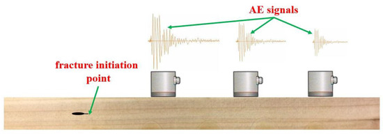
Figure 1.
Attenuation of acoustic emission signals during propagation.
Some literatures [17,46] have shown that, when the propagation distance becomes larger, the attenuation of the acoustic emission signal in the propagation process is a non-negligible influencing factor. However, this study needs to obtain the intensity of the AE signals at the sound source for verifying the accuracy of Formula ().
This paper chose Chinese fir with a moisture content of about 10% and density of 0.306 g/cm3, and the Chinese fir is processed into the 300 mm × 20 mm × 20 mm wooden beam test samples. A total of 5 samples were made, and the results were averaged. In order to avoid different sensitivities of the frequency response of the signals received by different sensors, this test used two sensors (No.53005 and No.53006, respectively) to alternate the pencil lead breaking tests, and the test scheme is shown in Figure 2.
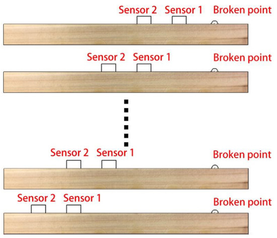
Figure 2.
Lead breaking test scheme.
As shown in Figure 2, the position of the broken point on the right is kept unchanged every time, and Sensors 1 and 2 are moved synchronously to the left with a step size of 25 mm. At the same time, in order to eliminate the influence of the pencil core quality and lead breaking angle on the accuracy of the results, the lead breaking times of each lead breaking test should not be less than 4 times. Then, select the AE signal with spectrum characteristics greater than 100 kHz as the effective signal [46].
An acoustic emission signal analyzer 8-channel system (from Beijing Softland Times Scientific & Technology Co. Ltd, Beijing, China) was used to gather the AE signals (see Figure 3). The AE signals were measured with SR-150 piezoelectric sensor in the 50–400 kHz frequency range. The acoustic signals were amplified with a gain of 40 dB. The acoustic signals were acquired with a sampling rate of 3 MHz by means of an acoustic emission analyzer. Thirty millivolts was selected as the threshold voltage to trigger the permanent storage of the AE signals [25].
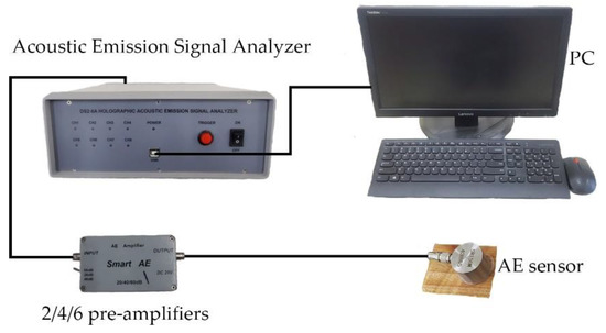
Figure 3.
A diagram to show the instrument connection for the acoustic emission.
3.2. Tensile Tests of Double Cantilever Beam
It can be known from Formula () that, if the acoustic emission parameters are to be used to judge the crack condition, the energy release rate () and undetermined coefficient (C) need to be known in advance. For the test method of the energy release rate () of a mode I fracture within the wood, a double cantilever beam sample is often used, which is calculated by measuring the flexibility. Triboulot et al. [47] used this method to calibrate the fracture toughness of wood with TL cracks, and compared with the finite element solution, the results were in good agreement. Therefore, the purpose of this test is to obtain the energy release rate () and undetermined coefficient (C) of the Chinese fir specimens by the double cantilever beam (DCB) test.
This paper selected apparently clean heartwood areas with straight textures to prepare the double cantilever beams (DCB). According to ASTM D3433-75 (1985), specimens in form of cuboids with dimensions of 200 (longitudinal) × 20 (tangential) × 20 (radial) mm3 were cut (Figure 4a).
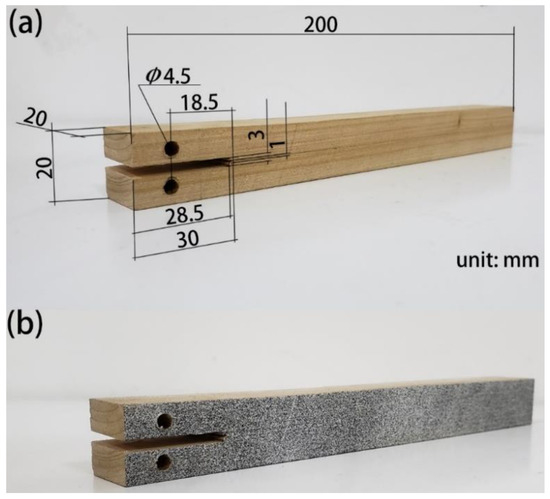
Figure 4.
(a) Double cantilever beam (DCB) in view of mode I. (b) Double cantilever beam (DCB) in view of mode I after painting the speckle.
In order to load the specimen, 4.5-mm-diameter holes were drilled into each sample above and below. According to Pleschberger’s literature [48], in order to focus the crack tip propagation on the cross-sectional area, a crack with a depth of 28.5 mm was processed by a 3-mm saw blade, and then, a razor blade was used to draw a depth of 30 mm.
Since the crack tip needed to be located during the mechanical test in the fracture analysis, the digital image correlation (DIC) method is adopted in this paper, which can provide highly accurate crack tip locations [49,50]. So, matte paint was used to paint speckles on the surface of the specimen (Figure 4b), which had been proved to be effective in Ritschel’s paper [36]. The position information of the crack tip was obtained by a CCD camera (Figure 5b).
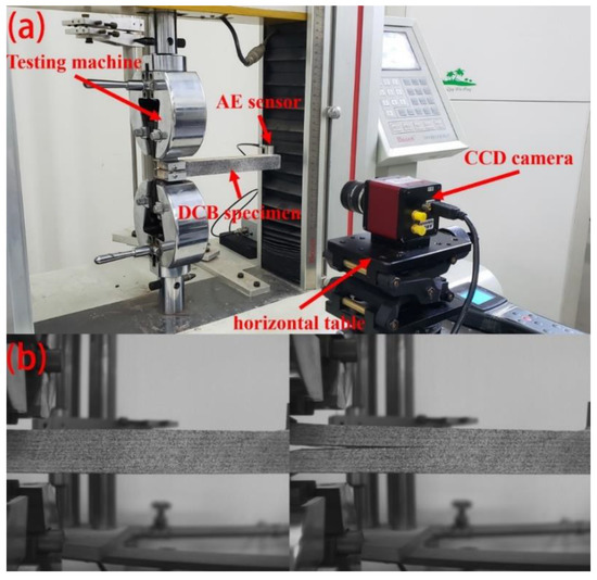
Figure 5.
(a) Test device schematic. (b) Crack growth tracking. CCD.
As shown in Figure 5a, the CCD camera was fixed on the test bench, and the distance was adjusted so that the lens was 500 mm from the test piece. During the test, the DIC system camera took images at a frequency of 2 Hz. As soon as the load dropped, the location of the crack tip was recorded as Li (i = 1,2,3…), and the crack propagation length was recorded as ai (i = 1,2,3…), as shown in Figure 6. An acoustic emission sensor was placed at the end of the specimen to record the acoustic emission signals generated during the crack propagation. Acoustic emission parameter settings were the same as Section 3.1.
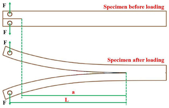
Figure 6.
The difference between a and L. F.P.S.: F is external load.
After clamping the specimen into the testing machine (Reger, Shenzhen, China), the test specification was configured with a 2-mm/min displacement velocity during real sampling time. When the mechanical testing machine begins to load, the acoustic emission instrument and the CCD camera also begin to acquire acoustic signals and images, respectively. Testing was interrupted, and the data was stored, if a sudden drop in force of 50% of the maximum load appeared. At the same time, the crack tip location was recorded as Li (i = 1,2,3…) and the AE activity. Then, it was loaded again based on the same rules, and the cycle continued until the specimen was completely broken.
4. Results and Discussion
4.1. Acoustic Emission Signal Attenuation Characteristics in Chinese Fir
As described in Section 3.1, the data is processed using the relative amplitude attenuation rate after the test is completed. The formula is as follows:
where is the amplitude value obtained by Sensor 1, and is the amplitude value obtained by Sensor 2. The data is processed to get a scatterplot, as shown below (Figure 7).
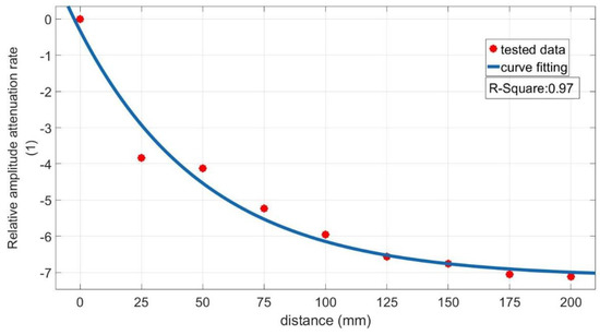
Figure 7.
Relationship between relative amplitude attenuation rate and the propagation distance.
The red dot in the figure is the relative amplitude attenuation rate obtained through the experiments. Observing Figure 7 shows that, as the propagation distance of the acoustic signal increases, the degree of attenuation also increases. It shows that the propagation distance has a great influence on the signal amplitude. This change trend is approximately in the form of an index, so the relationship between the propagation distance and the relative amplitude attenuation rate is obtained by fitting in this paper:
where is the distance from the sensor to the sound source, and is the relative amplitude attenuation rate from the sound source .
Knowing and , we can use Formula () to obtain the relative attenuation rate (which can be used as a compensation coefficient) when the distance x is between the sound source and the sensor. Then, according to Formula (), the amplitude of the AE signal at a distance of x millimeters from the jth sensor can be calculated, providing the calculation basis for determining the value at the sound source below.
4.2. Tensile Tests Analysis of Double Cantilever Beam
4.2.1. Determine the Energy Release Rate ()
As described in Section 3.2, the displacement load curves of several Chinese fir test pieces were obtained after the test was completed, as shown in Figure 8a.
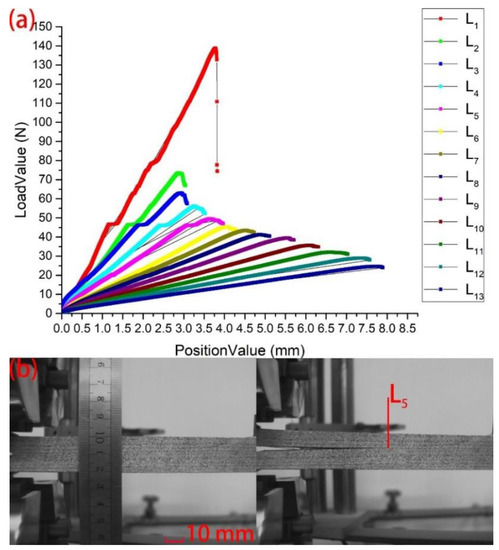
Figure 8.
(a) The displacement load curve of Chinese fir test specimens, where “PositionValue” refers to the displacement. (b) Image calibration and crack monitoring.
In Figure 8, as soon as the crack rapidly grew and the load dropped, the loading was stopped immediately, and the data were saved. At the same time, the location of the crack tip was marked by means of the DIC. Finally, we reset the test machine so that the load is zero. We repeated the above process until the specimens were broken completely. After the tests, according to the camera calibration and the length of the crack in the image (Figure 8b), we calculated the length of the crack () on the sample. From the displacement load curve, it can be seen that each curve basically maintains a straight state, so it can be explained that the fracture of Chinese fir in the longitudinal is approximately brittle. In addition, in the crack in the longitudinal direction of the test piece cracks, the crack growth basically belongs to the unsteady state, and the bearing capacity of the test piece decreases rapidly. According to Pleschberger’s research [51], the highest point of each curve represents the critical point of rapid crack growth, because the critical value Fcrit = Fmax can be determined. The slope of the straight line segment of each displacement load curve is inversely proportional to the crack length, and the inverse of the slope is the compliance of the specimen corresponding to the different crack length.
Table 1 shows the size of the Chinese fir specimen and the corresponding test values Fmax and flexibility C when the crack length extends to Li.

Table 1.
Dimensions and test data of the double cantilever beam (DCB (test piece (TL crack).
The flexibility corresponding to location of the crack tip of the same specimen can be obtained from Table 1. An exponential equation can be used to describe the relationship between the crack body and (as shown in Figure 9).
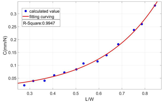
Figure 9.
Flexibility curve of the Chinese fir test piece.
Using the regression equation and Formula (), two undetermined coefficients can be obtained (q = 0.014; p = 4.044).
The crack propagation resistance (or fracture toughness) of a material can be calculated as follows:
where B = 20 mm, and W = 200 mm.
Figure 10 shows that a scatterplot of the relationship between the energy release rate () and different crack lengths (ai) obtained by using Formula (). The calculated by Formula () was averaged, and the final average value was regarded as the energy release rate of the fracture mode I within the Chinese fir. The ordinate value of the red line in the figure is the result of averaging all data, which is = 121.34 J/m2.
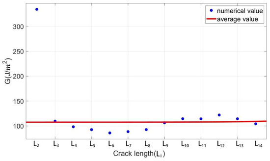
Figure 10.
Relationship between the energy release rate () and Li in the Chinese fir DCB specimen.
4.2.2. Determine the Undetermined Coefficient (C)
The was calculated in this paper, and a method to calculate the amplitude of the sound source signal by the signal received by the sensor was obtained. Then, based on is the sum of the squares of , so as to obtain . Next, the value of the undetermined coefficient C in Formula () is determined in this paper.
As described in Section 3.2, the AE sensor received the signals at each crack growth. Therefore, Formulas (6), (), and () can be sued to calculate the value when the crack growth length is ai, as shown in Figure 11.
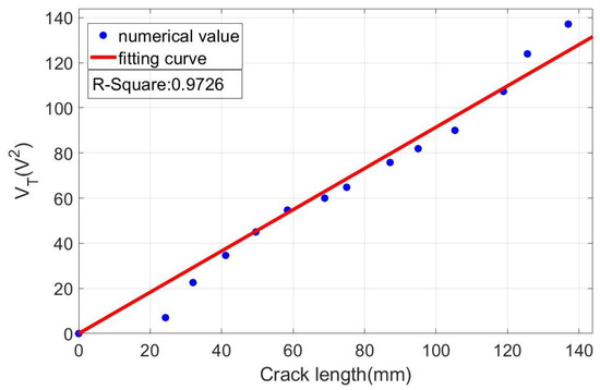
Figure 11.
Relationship between the crack propagation length and voltage ().
As shown in Figure 10, after compensating for the attenuation of the acoustic emission signal during propagation, the crack propagation length and VT approximately show a linear relationship. At the same time, it can also be proven that the form of Formula () is consistent with the actual test situation. Therefore, after transforming Formula (), we get:
It can be known from the above formula and Figure 11 that there is a linear relationship between the and crack length a, so using above formula to fit the scattered points can be obtained:
where B = 20 mm, and 0.12134 N/mm. So, the calculation result is = 2.637. Therefore, the crack instability prediction model can be obtained by substituting the known parameters into Formula ().
4.3. Validation of Formulas and Analysis
4.3.1. Validation of Formulas
In order to verify the rationality and effectiveness of the mode established, the (denoted as ) calculated by the model was compared with the the (denoted as ) calculated from test data under the same crack length. The test materials and method were the same as described in Section 3.2. Four samples were used in this experiment, and the results were averaged. The crack length ai was calculated by the DIC method. was calculated according to Formula (). According to the amplitude of the signal received by AE sensor, Formulas (6), (), and () were substituted to calculate the when the crack growth length was ai. Comparing the and , the results are shown in Figure 12.
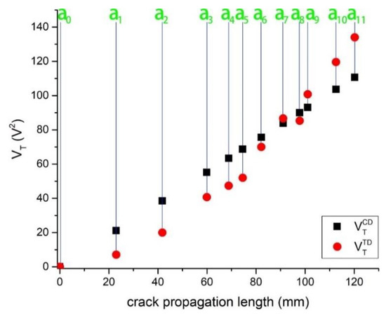
Figure 12.
Relationship between the velocity calculated by the model () and the velocity calculated by the test data (). The correlation coefficient was 0.96.
As shown in Figure 12, the black box represents the value of the calculated by the model when the crack growth length is ai, denoted as . The red circle represents the value of the calculated by the test data received by the AE sensor when the crack growth length is ai, denoted as . As can be seen from Figure 12, the model results have a high degree of agreement with the experimental value of the , and its correlation coefficient is 0.96, which is highly correlated. Therefore, the accuracy of the model was proved.
4.3.2. Optimization of AE sensor Layout Scheme
Further, after comparing the two sets of data, it was found that the was lower than the at the early stage of crack propagation. According to Section 4.1, at the early stage of crack propagation, the AE sensor was far from the crack tip (Figure 13a); that is, far from the signal source. In the propagation process, some low-amplitude and high-frequency signals were not received by the AE sensor due to attenuation. This can explain why the was lower than the at the beginning of the crack propagation.
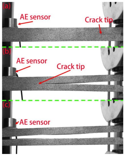
Figure 13.
Distance between the AE sensor and crack tip.
Similarly, the was higher than the at the later stage of crack propagation. This is because the AE sensor was relatively close to the crack tip (Figure 13b) and could receive more low-amplitude, high-frequency signals. Moreover, in the later stage of crack propagation, after the end of each crack propagation, there were still redundant vibrations in the specimen (Figure 13c), and these signals were also received by the AE sensor. So, in the later stage of the experiment, the was higher than the .
Combined with the analysis of Figure 12, it can be seen that the crack growth length is in the range of a6 to a9, and the is the closest to the . In this range, the AE sensor can receive as many weak signals as possible, while avoiding the unwanted vibrations caused by the crack growth. Therefore, based on the distance from a6–a9 to the AE sensor, the monitoring distance of the AE sensor should be controlled at about 50 mm for the cantilever beam specimen.
4.3.3. Importance of the Early Warnings of Crack Growth
In addition, this paper compared the change amount () for each crack growth. As shown in Figure 14, ai represent the crack growth length, and is the difference between the two adjacent growth lengths; that is, the change amount of a single crack.
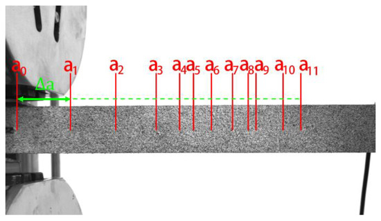
Figure 14.
Distance between the .
Based on the analysis of Figure 12 and Figure 14, it can be seen that, in the early stage of the test, the is relatively large, while, in the later stage of the test, the is significantly reduced. From a global perspective, the change amount () of each crack growth showed a trend of decreasing during the test.
According to the analysis of Figure 14, the maximum load Fmax that forced the crack to grow at the early stage of the test was also significantly higher than that at the later stage of the test. From the point of view of energy, it means that the external load has done more work on the specimen, compared with the later stage of the test. For Chinese fir, the energy required for crack propagation per unit area is fixed; that is, is constant. According to the law of the conservation of energy, the work done by the external load is used for crack growth. This also explains why the change amount of each crack propagation is larger in the early stage of the test than in the later stage of the test. This phenomenon also illustrates the importance of early warnings of crack growths in the field of wood health monitoring and the necessity of the work in this paper.
4.3.4. Method of Using Crack Instability Prediction Model
The purpose of this section is to explain the specific usage of the model. The test material and the sample dimensions are the same as described in Section 3.2. A random length of crack was premade on the DCB sample by the loading of the test machine (Figure 15a). When the material is unchanged, and C are known quantities. Based on Formula (16), the acceptable damage area “S” (S = aB) should be determined according to the actual situation. The setting of the area requires a comprehensive consideration of factors such as the size of the test piece, the distance between the loading point and the crack tip, and the individual’s tolerance for damage. Based on experience, set the maximum acceptable damage area to 200 mm2. Here, 200mm2 refers to the sum of all the microdamage areas distributed in the damage area. According to Formula (16), calculate the VT value and use it as the threshold value (denoted as ). The test was interrupted and the data was stored if there was a sudden load drop or crack growth (Figure 15b).
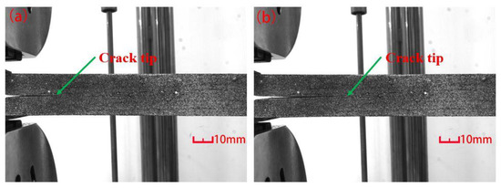
Figure 15.
(a) DCB specimen before the formal test. (b) DCB specimen after the test.
It can be seen from the distribution diagram (Figure 16) of the acoustic emission amplitude that, in the early stage of the test, the specimen is in the elastic stage, and there is barely an acoustic emission signal. In the middle stage of the test, the acoustic emission signals began to appear, at which time, new microcracks began to appear in the wood. As the load continued to increase, the number of acoustic emissions gradually increased, new microcracks were continuously generated inside the material, and then, the microcracks converged to form macrocracks. Eventually, it led to the destruction of the sample.
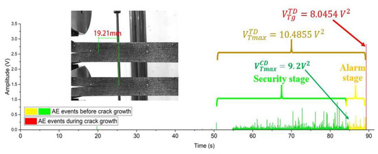
Figure 16.
Acoustic emission amplitude-time distribution.
As shown in Figure 16, the green and yellow rectangles are the amplitude distribution of the DCB sample before the crack growth. The red rectangle is the amplitude distribution during the crack growth, where is the VT value during the crack growth. According to Formula (16), the values of and can be obtained (Figure 16). It can be seen from Figure 16 that the stage before reaching the threshold value is the safety stage. Although there are increasing micro damages at this time, it does not pose a threat to the sample. When VT = , the model will send an early warning signal, and the specimen will enter the alarm stage. If the load is stopped immediately, the crack will not grow. However, the specimen is already in a state of severe damage at this time. If the threshold is set lower, the specimen can be better protected. Therefore, by setting the threshold value, the crack instability prediction model can provide early warnings of impending damage and can avoid personal injury and property damage. On the other hand, the crack instability prediction model can be used to realize real-time understanding of wood damage through the observation of acoustic emission parameters. Conversely, the model has some limitations. First of all, you need to have some experience in setting the threshold. Secondly, the sensors layout should be reasonable, which requires the location of the crack tip to be known. If the crack tip is inside the material, the current solution is to arrange the sensor matrix. The main problem to be solved next in this work is the determination of the internal damage source of the wood.
5. Conclusions
In this paper, the propagation characteristics of acoustic emission signals within Chinese fir and the energy conversion of a mode I fracture within Chinese fir were studied. At the same time, the acoustic emission technology and digital image correlation method were used for monitoring, and the AE parameters was used to reflect whether the crack was stable. The specific research conclusions are as follows:
- The attenuation characteristics of the acoustic emission signals in Chinese fir were obtained through a lead breaking test; that is, the attenuation degree of the acoustic emission signals increased exponentially as the propagation distance increased. The relationship between the relative amplitude attenuation rate and the propagation distance of the acoustic emission signal was established by the regression method. When the position of the sound source was known, the actual strength of the signal at the sound source could be estimated through the compensation coefficient (relative amplitude attenuation rate).
- Under uniaxial stress, the acoustic emission parameters obtained in the test showed different characteristics in each stage of the test. Among them, in the early stage of the test, the was higher than the . On the contrary, in the later stage, the was lower than the . Thus, for the cantilever beam specimen, the optimal location of the AE sensor should be about 50 mm away from the crack tip. Moreover, the length of the crack growth in the early stage was longer than that in the later stage, so it was particularly important to monitor the crack growth in the early stage.
- Combining the thermodynamic approach with acoustic emission technology, a crack instability prediction model was derived. The accuracy of this model was verified by using the tensile test of the double cantilever beam specimens. The model realized that the state information of crack stability can be obtained by monitoring the acoustic mission parameter (). The established mode and relationship form were simple, and the relevant parameters were easy to obtain. After verification, the model had highly accuracy, which proved the rationality and validity of the model established. In the future, this study may consider conducting research on more complicated damage forms.
Author Contributions
D.Z., J.Z., and Q.Z. conceived this study, and Q.Z. conducted the experiments. Q.Z. and J.Z. implemented and analyzed the experimental results. Q.Z. and D.Z. wrote the manuscript. All authors have read and agreed to the published version of the manuscript.
Funding
This research was funded by the Beijing Natural Science Foundation, grant number 2182045.
Acknowledgments
We are grateful to Jianzhong Zhang from Beijing Forestry University, Beijing, China for his help with the laboratory analysis work.
Conflicts of Interest
The authors declare no conflict of interest.
References
- Elias, P.; Boucher, D. Planting for the Future. How Demand for Wood Products Could Be Friendly to Tropical Forests. Available online: https://www.ucsusa.org/resources/planting-future (accessed on 13 April 2020).
- Sen, N.; Kundu, T. A new wave front shape-based approach for acoustic source localization in an anisotropic plate without knowing its material properties. Ultrasonics 2018, 87, 20–32. [Google Scholar] [CrossRef]
- Yin, S.X.; Cui, Z.W.; Kundu, T. Acoustic source localization in anisotropic plates with “Z” shaped sensor clusters. Ultrasonics 2018, 84, 34–37. [Google Scholar] [CrossRef]
- Zhao, X.M.; Jiao, L.L.; Zhao, J.; Zhao, D. Acoustic emission attenuation and source location on the bending failure of the rectangular mortise-tenon joint for wood structures. J. Beijing For. Univ. 2017, 39, 107–111. [Google Scholar] [CrossRef]
- Ye, G.Y.; Xu, K.J.; Wu, W.K. Multivariable modeling of valve inner leakage acoustic emission signal based on Gaussian process. Mech. Syst. Signal Process. 2020, 140, 106675. [Google Scholar] [CrossRef]
- Liu, C.; Wu, X.; Mao, J.L.; Liu, X.Q. Acoustic emission signal processing for rolling bearing running state assessment using compressive sensing. Mech. Syst. Signal Process. 2017, 91, 395–406. [Google Scholar] [CrossRef]
- Butterfield, J.D.; Krynkin, A.; Collins, R.P.; Beck, S.B.M. Experimental investigation into vibro-acoustic emission signal processing techniques to quantify leak flow rate in plastic water distribution pipes. Appl. Acoust. 2017, 119, 146–155. [Google Scholar] [CrossRef]
- Wisner, B.; Mazur, K.; Perumal, V.; Baxevanakis, K.P.; An, L.; Feng, G.; Kontsos, A. Acoustic emission signal processing framework to identify fracture in aluminum alloys. Eng. Fract. Mech. 2019, 210, 367–380. [Google Scholar] [CrossRef]
- Xu, J.; Wang, W.X.; Han, Q.H.; Liu, X. Damage pattern recognition and damage evolution analysis of unidirectional CFRP tendons under tensile loading using acoustic emission technology. Compos. Struct. 2020, 238, 11928. [Google Scholar] [CrossRef]
- Kharrat, M.; Placet, V.; Ramasso, E.; Boubakar, M.L. Influence of damage accumulation under fatigue loading on the AE-based helth assessment of omposite materials: Wave distortion and AE-features evolution as a function o damage level. Compos. Part A Appl. Sci. Manuf. 2018, 109, 615–627. [Google Scholar] [CrossRef]
- Bucur, V. Acoustics of Wood; CRC Press: Boca Raton, NY, USA, 1995; p. 221. Available online: http://www.doc88.com/p-0478327166760.html (accessed on 2 November 2019).
- Booker, J.D.; Doe, P.E. Acoustic emission related to strain energy during drying o eucalyptus regnans boards. Wood Sci. Technol. 1995, 29, 145–156. [Google Scholar] [CrossRef]
- Schniewing, A.P.; Quarles, S.L.; Lee, S.H. Wood fracture, acoustic emission, and the drying process Part 1. Acoustic emission associated with fracture. Wood Sci. Technol. 1996, 30, 273–281. [Google Scholar] [CrossRef]
- Lee, S.H.; Qurales, S.L.; Schniewind, A.P. Wood fracture, acoustic emission, and the drying process Part 2. Acoustic emission pattern recognition analysis. Wood Sci. Technol. 1996, 30, 283–292. [Google Scholar] [CrossRef]
- Kowalski, S.J.; Molinski, W.; Musielak, G. The identification of fracture in dried wood based on theoretical modelling and acoustic emission. Wood Sci. Technol. 2004, 38, 35–52. [Google Scholar] [CrossRef]
- Jakiela, S.; Bratasz, L.; Kozlowski, R. Acoustic emission for tracing the evolution of damage in wooden objects. Stud. Conserv. 2007, 52, 101–109. Available online: https://www.jstor.org/stable/20619490 (accessed on 1 November 2019).
- Jakiela, S.; Kozlowski, B.R. Acoustic emission for tracing fracture intensity in lime wood due to climatic variations. Wood Sci. Technol. 2008, 42, 269–279. [Google Scholar] [CrossRef]
- Zhao, Q.; Zhao, D.; Zhao, J.; Fei, L.H. The Song Dynasty Shipwreck Monitoring and Analysis Using Acoustic Emission Technique. Forests 2019, 10, 767. [Google Scholar] [CrossRef]
- Berg, J.E.; Gradin, P.A. Effect fo temperature on fracture of spruce in compression, investigated by use of acoustic emission monitoring. J. Pulp Pap. Sci. 2000, 26, 294–299. [Google Scholar] [CrossRef]
- Reiterer, A.; Stanzl-Tschegg, S.E.; Tschegg, E.K. Mode I fracture and acoustic emission of softwood and hardwood. Wood Sci. Technol. 2000, 34, 417–430. [Google Scholar] [CrossRef]
- Aicher, S.; Hofflin, L.; Dill-Langer, G. Damage evolution and acoustic emission of wood at tension perpendicular to fiber. Holz als Roh und Werkstoff. 2001, 59, 104–116. [Google Scholar] [CrossRef]
- Chen, Z.; Gabbitas, B.; Hunt, D. Monitoring the fracture of wood in torsion using acoustic emission. J. Mater. Sci. 2006, 41, 3645–3655. [Google Scholar] [CrossRef]
- Varner, D.; Cerny, M.; Fajman, M. Possible sources of acoustic emission during static bending test of wood specimen. Acta Univ. Agric. Mendel. Brun. 2012, 60, 199–206. [Google Scholar] [CrossRef]
- Diakhate, M.; Bastidas-Aeteage, E.; Pitti, R.M.; Schoefs, F. Cluster analysis of acoustic emission activity within wood material: Towards a real-time monitoring of crack tip propagation. Eng. Fract. Mech. 2017, 180, 254–267. [Google Scholar] [CrossRef]
- Ando, K.; Hirashima, Y.; Sugihara, M.; Hirao, S.; Sasaki, Y. Microscopic processes of shearing fracture of old wood, examined using the acoustic emission technique. Jpn Wood Res. Soc. 2006, 52, 483–489. [Google Scholar] [CrossRef]
- Wu, Y.; Shao, Z.P.; Wang, F.; Tian, G.L. Acoustic emission characteristics and felicity effect of wood fracture perpendicular to the grain. J. Trop. For. Sci. 2014, 26, 522–531. [Google Scholar] [CrossRef]
- Diakhate, M.; Angellier, N.; Pitte, M.R.; Dubois, F. On the crack tip propagation monitoring within wood material: Cluster analysis of acoustic emission data compared with numerical modelling. Constr. Build. Mater. 2017, 156, 911–920. [Google Scholar] [CrossRef]
- Diakhate, M.; Bastidas-Arteaga, E.; Pitti, R.M.; Schoefs, F. Probabilistic improvement of crack propagation monitoring by using acoustic emission. In Fracture, Fatigue, Failure and Damage Evolution; Springer: Cham, Germany, 2017; Volume 8, pp. 111–118. [Google Scholar] [CrossRef]
- Yamaguchi, I. A Laser-specker strain gauge. J. Phys. E Sci. Instrum. 1981, 14, 1270–1273. [Google Scholar] [CrossRef]
- Peters, W.H.; Ranson, W.F. Digital imaging techniques in experimental stress analysis. Opt. Eng. 1982, 21, 427–431. [Google Scholar] [CrossRef]
- Jeong, G.Y.; Hindman, D.P. Orthotropic properties of loblolly pine (Pinus taeda) strands. J. Mater. Sci. 2010, 45, 5820–5830. [Google Scholar] [CrossRef]
- Ozyhar, T.; Hering, S.; Niemz, P. Moisture-dependent orthotropic tension-compression asymmetry of wood. Holzforschung 2013, 67, 395–404. [Google Scholar] [CrossRef]
- Milch, J.; Brabec, M.; Sebera, V.; Tippner, J. Verification of the elastic material characteristics of Norway spruce and European beech in the field of shear behaviour by means of digital image correlation (DIC) for finite element analysis (FEA). Holzforschung 2017, 71, 405–414. [Google Scholar] [CrossRef]
- Jiang, J.L.; Bachtiar, E.V.; Lu, J.X. Moisture-dependent orthotropic elasticity and strength properties of Chinese fir wood. Eur. J. Wood Wood Prod. 2017, 75, 927–938. [Google Scholar] [CrossRef]
- Ritschel, F.; Brunner, A.J.; Niemz, P. Nondestructive evaluation of damage accumulation in tensile test specimens made from solid wood and layered wood materials. Compos. Struct. 2013, 95, 44–52. [Google Scholar] [CrossRef]
- Ritschel, F.; Zhou, Y.; Brunner, A.J.; Fillbrandt, T.; Niemz, P. Acoustic emission analysis of industrial plywood materials exposed to destructive tensile load. Wood Sci. Technol. 2014, 48, 611–631. [Google Scholar] [CrossRef]
- Lamy, F.; Takarli, M.; Angellier, N.; Doubois, F.; Pop, O. Acoustic emission technique for fracture analysis in wood materials. Int. J. Fract. 2015, 192, 57–70. [Google Scholar] [CrossRef]
- Griffith, A.A. The phenomenon of rupture and flow in solid. Philos. Trans. R. Soc. Lond. Ser. A 1920, 221, 163–198. [Google Scholar]
- Engelder, T.; Fischer, M.P. Loading configurations and driving mechanisms for joints based on the Griffith energy-balance concept. Tectonophysics 1996, 256, 253–277. [Google Scholar] [CrossRef]
- Larsen, H.J.; Gustafsson, P.J. The fracture energy of wood in tension perpendicular to the grain. In Proceedings of the 23rd Meeting of W018, Lisbon, Portugal, 1 September 1990; pp. 1–6. [Google Scholar]
- Stanzl-Tschegg, S.E.; Tschegg, E.K.; Teischinger, A. Fracture energy of spruce wood after different drying procedures. Wood Fiber Sci. 1994, 26, 467–478. [Google Scholar] [CrossRef]
- Wang, Z.Q.; Chen, S.H. Advanced Fracture Mechanics; Science Press: Beijing, China, 2019; ISBN 9787030230355. [Google Scholar]
- Shen, G.T.; Geng, R.S.; Liu, S.F. Parameter analysis of acoustic emission signals. Non-Destr. Test. 2002, 24, 72–77. [Google Scholar] [CrossRef]
- Ji, H.G.; Jia, L.H.; Li, Z.D. Study on the AE-model of concrete damage. Acta Acust. 1996, 21, 601–608. [Google Scholar] [CrossRef]
- Fan, T.Y. Fracture Theory; Science Press: Beijing, China, 2003; ISBN 7-03-0100994-5. [Google Scholar]
- Xu, J.; Li, Y.; Tian, A.X.; Qu, J.M. Experimental research on size effect of acoustic emission location accuracy. Chin. J. Rock Mech. Eng. 2016, 35, 2826–2835. [Google Scholar]
- Triboulot, P.; Jodin, P.; Pluvinage, G. Validity of fracture mechanics concept applied to wood by finit element calculation. Wood Sci. Technol. 1984, 18, 448–455. [Google Scholar] [CrossRef]
- Feng, H.X.; Yi, W.J. Propagation characteristics of acoustic emission wave in reinforced concrete. Results Phys. 2017, 7, 3815–3819. [Google Scholar] [CrossRef]
- Rethore, J.; Roux, S.; Hild, F. An extended and integrated digital image correlation technique applied to the analysis of fracture samples. Eur. J. Comput. Mech. 2009, 18, 285–306. [Google Scholar] [CrossRef]
- Pop, O.; Meite, M.; Dubois, F.; Absi, J. Identification algorithm for fracture parameters by combining DIC and FEM approaches. Int. J. Fract. 2011, 170, 101–114. [Google Scholar] [CrossRef]
- Pleschberger, H.; Hansmann, C.; Muller, U.; Teischinger, A. Fracture energy approach for the identification of changes in the wood caused by the drying processes. Wood Sci. Technol. 2013, 47, 1323–1334. [Google Scholar] [CrossRef]


© 2020 by the authors. Licensee MDPI, Basel, Switzerland. This article is an open access article distributed under the terms and conditions of the Creative Commons Attribution (CC BY) license (http://creativecommons.org/licenses/by/4.0/).