Assessing Post-Harvest Regeneration in Northern Hardwood and Mixedwood Stands: Evolution of Species Composition and Dominance within 15-Year-Old Group Selection and Patch Cutting

Abstract

Multi-cohort forest management in northern hardwood stands may well be the best way to successfully regenerate tree species of intermediate shade tolerance, such as yellow birch (Betula alleghaniensis Britt.). The creation of large enough gaps in the canopy favors increased light availability within the opening, while soil scarification provides suitable germination seedbeds. Evidence of these methods’ success nonetheless remains mostly the purview of experimental studies rather than operational tests. In Quebec, Canada, the multi-cohort methods promoted include group selection cutting and patch cutting. The present study tested their implementation at an operational scale and over a large territory in both hardwood-dominated and mixedwood stands. We assessed their efficacy in promoting natural regeneration of commercial hardwood trees, notably yellow birch and sugar maple (Acer saccharum Marsh.). We conducted regeneration surveys at 2, 5, 10, and 15 years after harvest. Overall, group selection and patch cuttings were successful in regenerating the target species. Yellow birch, for instance, showed a mean stocking around 60% and a mean sapling density around 3400 stems ha⁻¹ after 15 years. We compared several variables for measuring regeneration in early years, and found that the relative abundance, the stocking based on one stem per sampling unit, and the mean maximum height were good predictors of the relative presence of yellow birch and sugar maple in 15-year-old canopy openings. Using smaller sampling units (6.25 m² rather than 25 m²) and waiting until year 5 may be more useful for making such predictions. In addition, there was an important turnover in vertical dominance in these openings. Non-commercial woody competitors were frequently dominant in early years but were often replaced by commercial hardwoods, notably yellow birch. We propose certain thresholds for assessing the success of post-harvest regeneration and for evaluating the need for a cleaning treatment.

1. Introduction

Different variations of multi-cohort forest management that build on the concept of gap dynamics [1] have been increasingly considered as the most adequate way of naturally regenerating the temperate hardwood forest because they emulate natural disturbances [2], even though these methods have not been universally adopted [3]. Indeed, the main natural disturbances driving the succession dynamics of these forests are windthrows [4,5] and other tree-falls [6], e.g., related to individual tree deaths, which produce gaps in the canopy of small [7,8] to intermediate size and severity [9,10]. These disturbances still remain limited in comparison with the more severe disturbances such as fires and insect outbreaks that are common across the boreal biome. As such, large-scale clearcuts can rarely be used to emulate natural disturbances in order to favor natural regeneration of temperate hardwood stands [11].

Yet, the hardwood forest harbors a relatively high diversity of tree species, with distinct ecological niches and, notably, varying requirements for light—and a varying tolerance of shade [12,13]. As a result, species composition of a stand vary across the different stages of succession, and the regeneration patterns that are unique to each species composition require distinct silvicultural approaches [14]. For instance, late-successional, shade-tolerant species such as sugar maple (Acer saccharum Marsh.) and American beech (Fagus grandifolia Ehrh.) generally thrive under single-tree selection systems, because their germination and seedling development do not require much light reaching the ground of the understory [7,11,15,16], at least in comparison with less tolerant species. Species of intermediate shade tolerance, however, such as yellow birch (Betula alleghaniensis Britt.), northern red oak (Quercus rubra L.), or white pine (Pinus strobus L.), have been shown to need larger openings in the canopy to favor more light transmission to the forest floor [17,18,19]. Failing that, recruitment of these species remains quite low and they are eventually displaced from the stand [20,21,22]. Hence, other partial harvest methods have been developed centered on the creation of gaps of varying sizes in the canopy, including, but not limited to, group selection cutting [22,23], patch cutting [1], and more recently irregular shelterwood [24].

Evaluating the success of gap-based silvicultural systems in regenerating mid-tolerant tree species that are favored by neither clearcuts nor single-tree selection requires using measurements that will adequately predict the future stand composition. Management guidelines often define what proportions of a forest stand must be comprised of desirable tree species [25,26]. This requires a certain spatial homogeneity in seed dispersal, a good distribution of adequate germination microsites across the stand, and relatively high survival of established seedlings. Forest managers have long struggled to find adequate measurements to assess the success of post-harvest regeneration, be it natural or via plantation [27,28]. One widespread method nowadays is that of the ‘stocking’, also known as stocked quadrat method, which is the proportion of sampling units within a given area having at least one individual of the desired species [29]. In vegetation ecology, this concept is referred to as the ‘frequency’ of occurrence [30,31]. Thresholds for stocking may vary, for example values ranging from 40% [32] to 70% [28] or 80% [33] have been acknowledged as ‘fully stocked’, i.e., regenerated well enough that, based on expected stem density (trees ha⁻¹), a dense mature stand will eventually develop to replace the one that was harvested. Where forest management relies on natural regeneration to restock a forested area after harvest, the stocking is a measure of successful dispersion and germination of seeds, of adequate spatial distribution of seedlings, and finally of the early survival of seedlings.

Stem density is another measurement regularly employed to assess regeneration, especially in experimental studies. It can be the absolute number of stems per hectare, either of all species or of only one target species, or the relative proportion of a given species among all stems (then more akin to relative abundance). It may provide a more complete image of current stand conditions, although it is likely more time- and resource-consuming to compile in the field compared with stocking. In their silvicultural guide, Leak et al. [34] proposed stocking objectives for post-harvest, even-aged, northern hardwood stands. They advocated assessing dominant, free-to-grow stems from desirable species in plots 4–5.7 m² in size, and they defined ‘recommended stocking’ as 60% and ‘minimum stocking’ as 40%. Using their stocking diagram, these values correspond to densities around 1000 stems ha⁻¹ for minimum stocking (C line) and around 1500 stems ha⁻¹ for recommended stocking (B line) in order to eventually obtain full stocking at a mean diameter at breast height (DBH; measured at 1.3 m above the ground) of 10 cm (4 inches).

Although the post-harvest assessment of regeneration has been a staple of forestry operations for at least the last century, there are still few reliable methods to actually predict stand composition based on early assessments [29,35,36,37]. What these surveys aim at doing, theoretically, is informing forest managers whether the future presence of desirable tree species can be assured by natural regeneration, or whether other means must be taken (e.g., soil scarification, control of competitive vegetation, planting). Halpin et al. [38] simulated long-term development of northern hardwood stands after single-tree and group selection cutting, and reported that although intermediate shade-tolerant species such as yellow birch were more abundant in group-selection openings, there was still much variation, thus suggesting that the success of these harvesting methods in promoting regeneration was not automatic. Therefore, there is still a need to assess empirically and at an operational scale the efficacy of multi-cohort forest management in attaining its objective of naturally regenerating target species.

In Quebec, group selection and patch cuttings have been recommended as a way to naturally regenerate mid-tolerant and intolerant species in hardwood stands and mixedwood stands since the end of the 1990s [26]. This idea was based on experiments realized in hardwoods stands of the northeastern United States [39,40,41]. The main objective was to promote the natural regeneration of birches (yellow and paper birch (Betula papyrifera Marsh.)) in yellow birch-conifer and sugar maple-yellow birch forest types. Quebec’s management guidelines [26] suggested either harvested groups of 500 to 1500 m² or harvested patches of 1–2 ha in size, respectively covering 10% or 20% of the stand area at each cutting cycle. It was additionally suggested to partially harvest the forest matrix between groups and patches to improve stand quality and favor stand productivity. For both methods, it was also proposed to apply soil scarification within groups and patches in order to expose the mineral horizon or mix the organic and mineral horizons, thus creating adequate microsites for birch regeneration [42,43,44,45,46]. Since the introduction of these guidelines, short-term experimental results (5–6 years) have been published about group selection and patch cuttings with intentional or passive soil scarification in Quebec [9,47,48,49,50] that confirmed the effectiveness of these treatments’ combination to regenerate yellow birch, although they were applied only experimentally and at one or two sites per study.

The main objective of the present study was to evaluate the effectiveness of two multi-cohort treatments (group selection and patch cutting) applied operationally across the province of Quebec, Canada, at a large scale (Figure 1), at a great number of sites (n = 71), and at four successive points in time over a 15-year period. Specific objectives were two-fold: (1) to evaluate the success of post-harvest regeneration within group selection cutting and patch cutting; and (2) to assess the feasibility of predicting future species composition and dominance within regenerated openings based on measurements made in the early years after harvest.

2. Materials and Methods

2.1. Description of Study Sites

Study sites were established during the years 2000 through 2005 along an East-West gradient across the south of the province of Quebec, Canada (approximately between 47°57′ and 45°28′ N, and between 78°58′ and 70°11′ W), within hardwood (sugar maple-yellow birch) and mixedwood (balsam fir-yellow birch) forest stands (Figure 1). Altitude varies from 227 to 850 m above sea level (a.s.l.), with a mean = 414 m a.s.l. and standard deviation (SD) = 124. Mean annual temperature and precipitations are in the ranges of 0.7–4.1 °C and 912–1306 mm, respectively, for the reference period 1981–2010 [51]. Tree species composing the forest stands prior to harvest were mainly sugar maple and yellow birch for hardwood stands, or balsam fir (Abies balsamea (L.) Mill.), yellow birch, northern white cedar (Thuja occidentalis L.), and spruces (Picea glauca (Moench) Voss. or P. rubens Sarg.) for mixedwood stands. Main companion species were American beech, red maple (Acer rubrum L.), paper birch, trembling aspen (Populus tremuloides Michx.), American larch (Larix laricina [Du Roi] K. Koch), and eastern hemlock (Tsuga canadensis (L.) Carr.). The most common competing trees and shrubs encountered in the regeneration surveys included pin cherry (Prunus pensylvanica L.), striped maple (Acer pensylvanicum L.), mountain maple (Acer spicatum Lam.), beaked hazel (Corylus cornuta Marsh.), bush honeysuckle (Diervilla lonicera Mill.), hobblebush (Viburnum lantanoides Michx.), red elderberry (Sambucus pubens Michx.), wild raspberry (Rubus idaeus L.), and willows (Salix spp.).

For the purpose of this study, we selected 32 canopy openings established according to patch methods (where a rectangular area ranging from 1 to 2 ha is clear-cut; yet some patches in the present study were slightly smaller or larger, resulting in a realized range of 0.8–2.6 ha) and 117 openings created according to group selection practices (circular area of 500–1500 m²; Webster and Lorimer, 2002, 2005). Realized sizes of canopy openings averaged ≈1000 m² (SD = 300) for groups and 1.5 ha (SD = 0.6) for patches. Groups were spatially arranged in 39 clusters of three group openings each. Environmental conditions (e.g., topography, aspect, position on the slope, soil type, and drainage) were mostly homogeneous among openings of a same cluster, hence each cluster was treated as one replicate for the purpose of the present analyses. Canopy openings were established in locations where several mature seed trees of yellow birch would be present in the border of the opening. Within the canopy openings created by both group selection and patch cutting, all stems with a DBH ≥ 10 cm were cut and pulled out of the area. Distance between group openings was at least 30 m, while patches were separated by at least 50 m. There was also a 30-m minimum distance between a group or patch and any forest road. Forested areas around or between groups and patches were harvested according to single-tree selection methods. All selected canopy openings were part of a larger number of operationally harvested areas, and as such our selection was aimed at assessing long-term impacts of actual silvicultural operations across publicly owned forests in Quebec. Due to this aim, establishment of study sites was reliant on the rhythm of forestry operations; hence the 71 canopy openings (patches or group clusters) were added over the course of 6 years (2000–2005) at a relatively steady rate (mean number of new openings per year = 12, SD = 6).

Following harvest, soil scarification was undertaken in order to produce favorable germination seedbeds for yellow birch. The objective of scarification was to lightly disturb the upper organic layer (L and F horizons) and expose the upper mineral soil (B horizon), or to superficially mix the upper organic and mineral layers. Different types of machinery were used depending on their availability per region: (1) scarification using a skidder equipped with a rake blade, (2) scarification using a skidder with a standard blade, or (3) scarification by an excavator with a standard bucket. With the first two methods, the whole area of a canopy opening was treated. For the third method, scarification was rather done on multiple small spots across the opening, with each scarified spot ranging in size from 6 to 10 m² with a minimal width of 2 m corresponding to the bucket width [26]. It thus locally exposed the mineral soil and controlled the competing vegetation. The aim was that each scarified spot should present at least one 1-m² germination microsite. It was planned so as to obtain at least 150 scarified spots ha⁻¹ in group openings and 300 spots ha⁻¹ in patches. Among group-selection openings, soil scarification method n°2 was the most used, while method n°3 was the most common among patches. In a previous publication about these sites, Beaudet et al. [52] assessed the efficacy of scarification in creating suitable microsites. That assessment was conducted in year 0 (i.e., the same year as the harvest and scarification) in the same plots used in the present study (see next section). Overall, soil scarification was very successful in preparing germination seedbeds, with 70%, 40%, and 55% exposed mineral soil and disturbed litter for the three aforementioned scarification treatments, respectively. Since good seed crops usually occur at about 2- to 3-year intervals for yellow birch [43] and scarification was performed any year from 2000 to 2005, then some openings were sampled following a variety of seed crops for which we do not have a precise documentation.

2.2. Sampling Design

In each group or patch, a number of permanent, square-shaped, 5 × 5 m (25 m²) sampling plots were established. In the case of groups, a first plot was placed in the middle of the opening, followed by two more plots in each cardinal direction, thus forming a cross and totaling up to nine plots in a group opening. A distance of 7–10 m was kept between centers of neighboring plots (to optimize spatial coverage), hence some smaller group openings had fewer sampling plots (mean number of sampling plots per group = 7, SD = 2). In patches, sampling plots were positioned according to a 20 × 20 m grid overlay, with a 5-m buffer from the patch’s edges (mean number of sampling plots per patch = 32, SD = 10). Each plot was further divided into four quadrats of equal size (2.5 × 2.5 m, 6.25 m²).

Regeneration surveys were carried out in all quadrats of all sampling plots at fixed time steps, i.e., 2, 5, 10, and 15 years after initial harvest (but on varying calendar years because of different starting dates, as mentioned before). The first three surveys have sampled all 71 clusters; however, the fourth and last survey has only been conducted in 49 clusters so far because the rest have not yet reached 15 years of age. Statistical analyses had concordant sample sizes.

Surveys compiled abundance (number of stems) and height (maximum) of all tree- and shrub-like woody species (total of 44 species across all sites, see

Table 1. Tree and shrub species reported in the regeneration surveys across the study sites, as well as the species pools used in the analyses. Some species do not appear in this table because they were too rare.

Species or Species Pool	Common Name	Scientific Name
SM	Sugar maple	Acer saccharum
YB	Yellow birch	Betula alleghaniensis
PB	Paper birch	Betula papyrifera
INTOL, shade-intolerant, deciduous, commercial tree species	White ash	Fraxinus americana
	Black ash	Fraxinus nigra
	Bigtooth aspen	Populus grandidentata
	Trembling aspen	Populus tremuloides
	Red oak	Quercus rubra
	American basswood	Tillia americana
TOL, shade-tolerant, deciduous, commercial tree species	Red maple	Acer rubrum
	American beech	Fagus grandifolia
	American hop-hornbeam	Ostrya virginiana
CONIF, commercial coniferous tree species	Balsam fir	Abies balsamea
	American larch	Larix laricina
	White spruce	Picea glauca
	Black spruce	Picea mariana
	Red spruce	Picea rubens
	Red pine	Pinus resinosa
	White pine	Pinus strobus
	Northern white cedar	Thuja occidentalis
	Eastern hemlock	Tsuga canadensis
NCOM-tree, non-commercial woody species that can reach tree size	Striped maple	Acer pensylvanicum
	Mountain maple	Acer spicatum
	Pin cherry	Prunus pensylvanica
NCOM-shrub, non-commercial woody species that remain shrub-sized or small trees	Speckled alder	Alnus rugosa
	Serviceberry	Amelanchier canadensis
	Beaked hazel	Corylus cornuta
	Choke cherry	Prunus virginiana
	Staghorn sumac	Rhus typhina
	Willow	Salix spp.
	Black elderberry	Sambucus canadensis
	Red elderberry	Sambucus pubens
	American mountain-ash	Sorbus americana
	Canadian yew	Taxus canadensis

). Abundance was compiled distinctly for six ontogenetic stages: small seedlings (< 1 m-tall), large seedlings (≥ 1 m-tall), and saplings (four classes denominated according to their median DBH: 2, 4, 6, and 8 cm, respectively ranging from 1.1. to 3.0 cm, from 3.1 to 5.0 cm, and so forth). However, abundance for the small seedlings (< 1 m) was counted only up to 11 stems per quadrat, with additional stems being ignored. Moreover, the year-15 survey did not measure seedlings under 1 m in height, because the canopy was closing and these small seedlings had become marginal, as well as being unlikely to reach the canopy. Height was measured separately for two categories: seedlings and saplings. Maximum height corresponded to the height of the highest individual per species and per category.

Topographic, edaphic, and other environmental factors were compiled for individual canopy openings [53]. Slope was measured in the field with a clinometer, while altitude was computed from contour lines. Soil drainage was field-assessed visually by taking into account the slope, the position on the slope, as well as the soil type, depth, water content, and rockiness. Type of stand was defined in the field as ‘hardwood’ or ‘mixedwood’ when conifers comprised less than 25% or between 25% and 44% of the basal area, respectively.

2.3. Regeneration Indices

We computed several indices (see

Table 2. List of the 16 regeneration indices used in the present study, and their literary sources, when applicable.

Acronym	Full Name	Units	Source
BA	Basal area of the target species	m2 ha−1
BArel	Basal area of the target species Relative to the total basal area of all species combined	%
Stock-x	Stocking based on the presence of at least x stem of the target species, with x being equal to 1, 3, 5 or 10.	%	Beaudet et al., 2014 [52]
Stock-x, ≥1m	Stocking based on the presence of at least x stem of the target species, with x being equal to 1, 3, 5 or 10, and only considering stems ≥ 1 m in height	%	Beaudet et al., 2014 [52]
Stock-tallest	Stocking based on the target species being the tallest individual	%	Leak, 2007 [37]
Hmax	Maximum height, i.e., tallest individual of the target species	cm
Hmaxrel	Maximum height of the target species relative to the maximum height of the tallest other species	%
SIV	Species index value	Unitless, range = 0–1	Bohn and Nyland, 2003 [58]
StD	Stem density of the target species	Stems ha−1	Leak et al., 1987 [34]
%(species)	relative abundance, i.e., abundance of the target species relative to the total abundance of all species combined	%

) in order to assess regeneration success and to compare data from early vs. later surveys. Year-15 data played the role of the ‘future stand composition’, while both the year-2 and year-5 data were used as the ‘predictor composition’. The latter were chosen because that is when foresters expect, in case of unsuccessful or insufficient post-harvest regeneration, to be able to react in time with more intensive silvicultural interventions (e.g., competition control, further soil scarification, planting or seeding).

All indices were computed at the level of both sampling unit sizes (6.25 and 25 m²). In addition, distinct indices were calculated for all commercially exploited tree species, either individually or for several species combined in a pool based on a common trait (Table 1). Namely, indices were computed for yellow birch (YB), sugar maple (SM), paper birch (PB), the shade-intolerant, commercial, hardwood species pool (INTOL), the shade-tolerant, commercial, hardwood species pool (TOL), and the commercial coniferous species pool (CONIF). For certain specific analyses, we also created a pool comprising the three arborescent albeit non-commercial species that are the strongest competitors for the hardwoods (NCOM-tree, i.e., Acer pensylvanicum, A. spicatum, and Prunus pensylvanica), and one pool for the other non-commercial woody species that only attain shorter heights or remain shrub-like (NCOM-shrub, among others Corylus cornuta, Rubus idaeus, Sambucus pubens, and Viburnum lantanoides), thus posing less of a serious threat to commercial trees in the long term. Indeed, it has been shown that the latter have usually overtopped the smaller, shrub-like competitors by year 10 or 15 [32,54,55].

The stocking was included in the studied indices because it is so prevalent in forestry [33,35,56,57]. We computed it based on the presence of at least a certain number of individuals per sampling unit, either 1, 3, 5, or 10 individuals. These numbers were chosen based on previous analyses of the 5-year dataset from the same study sites [52], which tested stocking computations with a minimum number of individuals per sampling unit of 1, 5, 10, 15, 20, 25, or 30 individuals. It was shown that the largest drop in stocking value occurred between one and five individuals. Moreover, the advantage of the stocking method is its ease and speed of use in the field, but choosing numbers that are too high would mean that most if not all stems would have to be counted in a quadrat, which would be counter-productive. No distinction based on tree size or developmental stage was made in the case of stocking computations, thus all seedlings and saplings were considered. Nonetheless, it must be noted that small seedlings were not tallied in year 15, thus the stocking in that year included only seedlings ≥ 1 m in height and saplings.

We also selected additional indices based on a literature review (Table 2). These indices had to be computable with measurements available in our surveys, namely stem abundance, stem height, and species. DBH was not measured extensively in our openings (except for the rare trees > 9 cm in DBH that for some reason had not been cut during harvest), being mostly a way to categorize saplings, and as a result was only of limited usefulness.

We also used an index devised by Bohn and Nyland [58], the Species Index Value (SIV; Equation (1)), which compares the height × abundance (H × N) of a target species relative to the H × N of all woody species in a given sampling unit (Table 2).

$$SIV=\frac{{\sum }^{ }\left[H\times N\right]\mathrm{species}}{{\sum }^{ }\left[H\times N\right]\mathrm{sampling} \mathrm{unit}}$$

(1)

As abundance of small seedlings (< 1 m in height) was capped at 11 in these surveys, and because their impact on light interception was deemed marginal, they were excluded from SIV computations. In the case of saplings, because a single value of maximum height had been noted for all saplings in a quadrat (instead of one value per DBH class), further data manipulation was needed. Therefore, we filtered the data so as to keep only the sapling with the largest DBH per quadrat (hypothesizing that this individual would have been the one to provide the value for maximum height), then calculated mean values for maximum height per DBH class and per species (Table S1), and used these means for SIV computations. A linear regression built between mean maximum height and DBH for all species combined (n = 90) yielded a decent relationship (R-squared (R²) = 0.57, p < 0.0001).

A further index was built according to Leak’s [37] idea that the single dominant individual in a sampling plot would be the best predictor of future composition; hence, we added a stocking based on a target species being the tallest individual in the quadrat (rather than based on the simple presence of the species). This index was an indication of how often a species was vertically dominant in its vicinity. Being taller than its neighbors can be useful for developing seedlings and saplings in order to reach the canopy and access the light resource, although this is possibly less of an issue for species that are mid-tolerant or tolerant to shade.

In addition to the previous indices, we also added simpler indices based on stem density, relative abundance, as well as absolute (only the target species) and relative (to other species) values of maximum height and basal area. Maximum heights measured per 6.25-m² quadrat (with quadrats where the species was absent being given a height of 0 m) were averaged across the opening and finally averaged at the cluster level. It was thus rather a ‘mean of maximum heights’, but for the ease of reading will thereafter be referred to simply as ‘maximum height’. Stem density, which was calculated from the observed abundance of stems, excluded small seedlings (< 1 m) because of how their abundance was measured (as mentioned above for SIV). For basal area, large seedlings ≥ 1m in height were assumed to have a DBH of 0.5 cm, and saplings were assigned the mid-value of their respective DBH category (2 cm DBH for the 2-cm class, 4 cm DBH for the 4-cm class, and so forth). A given species’ relative abundance or relative basal area (expressed as percentages) compared that species’ absolute value to the sum of all species present in the sampling unit. Leak [37] similarly used a ‘percent basal area’, but which only comprised trees of DBH > 11.4 cm. For height, stem density, SIV, and basal area, values of 0 where given to sampling units where the species was absent.

2.4. Measuring Regeneration Success

Regarding measurable targets of regeneration success, Quebec’s management guidelines [26] advocate conducting a first survey 2–4 years after harvest, and a second one at 10–15 years, both based on 25-m² survey plots. In these surveys, the birches (yellow and paper—the main target species for such cuts in these guidelines) should present a stocking of at least 35% in groups and at least 60% in patches. Given the size of the suggested survey plots, this would correspond, respectively, to 140 and 240 well-distributed stems per hectare. With smaller, 6.25-m² quadrats, these stocking values would be 9% and 15%, respectively. In addition, the Quebec guidelines recommend that during the first post-harvest survey all commercial species combined should present a stocking of at least 80% (or 20% if using 6.25-m² quadrats). For the second survey, the guidelines specify that these stems should be free-to-grow small trees (seedlings, saplings, poles). Later, immediately after precommercial thinning (conducted when trees have attained heights between 5 and 7 m), the stocking for commercial species should be at least 60% and birches should amount between 250 and 500 future crop trees ha⁻¹. In comparison, using the stocking diagram of Leak et al. [34], a density of commercial species around 1000 stems ha⁻¹ would be judged as minimally successful (‘minimum stocking’, C line from Leak et al. [34]) and a density around 1500 stems ha⁻¹ as wholly successful (‘recommended stocking’, B line) in order to eventually obtain full stocking at a mean DBH of 10 cm (4 inches).

2.5. Statistical Analyses

In order to first assess the overall success of post-harvest regeneration across our study sites, we conducted analyses on the stocking based on one stem per sampling unit (Stock-1) and on stem density (StD, number of stems ha⁻¹). In the case of Stock-1 we focused solely on year-15 data (since early-year Stock-1 had already been analyzed by Beaudet et al. [52]), whereas data from all years were used for StD to evaluate its progression over time. Values per cluster were used for both Stock-1 and StD. The stocking in year 15 was the response variable in a linear mixed model using the species pool (Table 1), the type of canopy opening (group, patch), the type of stand (hardwood, mixedwood), and their interactions as fixed effects, and cluster as a random effect (to account for the different species within a cluster). Stem density was analyzed through a linear mixed model following a square-root transformation in order to meet expectations of normality and homoscedasticity of residuals. Fixed effects included the species pool, the type of canopy opening, the type of stand, the post-harvest year (2, 5, 10, and 15, as a continuous variable), the developmental stage (seedlings (≥ 1 m), saplings (all DBH combined)), and the interaction of each variable with post-harvest year (for the focus on changes of StD over time), while cluster was added as a random effect.

Then, regarding the various regeneration indices described in the previous section, the objective was to identify which index should be used in the first few years after harvest in order to predict future forest composition or, more appropriately in terms of forestry objectives, to predict the future dominant species. At the same time, we were also interested in finding which index would best represent said future composition. All indices were computed at the three time periods of interest (2, 5, and 15 years post-harvest), except basal area, which we limited to the 15-year data because we hypothesized it would be less useful at 2 and 5 years after harvest when many individuals barely reach 1.3 m in height. We compared the regeneration data from early years (2 and 5) to those of year 15 in a three-step procedure: (1) with correlations, to make a broad assessment of relationships between all indices, followed by (2) simple linear models using only the best-correlated indices identified in step 1, and finally (3) using a model selection approach that involved several environmental variables (defined in the next section).

Pearson correlations were conducted on all indices (k = 16, see Table 2) computed individually for each cluster (n = 49). A Bonferroni correction was applied to the resulting probability levels in order to account for multiple comparisons and to reduce chances of Type I errors [59]. As such, the significance threshold (α) used for the correlations was set at α = 0.05 and adjusted as follows:

$${\alpha }_{adj}=\frac{\alpha }{\left(2k\times \left(k-1\right)\right)/2}=\frac{0.05}{\left(32\times \left(16-1\right)\right)/2}=0.0002$$

(2)

The k values in Equation (2) reflect the fact that we were only interested in the correlations between years 2 and 15, and between years 5 and 15.

Linear regression models were constructed using indices calculated from year-15 data as the response variable and year-2 data as an explanatory variable. A certain number of categorical variables were added sequentially to build increasingly complex models: type of opening, type of stand, type of machinery used for soil scarification (skidder blade, skidder + rake, excavator), and their interactions. Model fit was assessed using the adjusted R² [60].

In order to assess the frequency at which vertical dominance in the early years after harvest was maintained over time, we performed a contingency analysis that compared the dominant (i.e., with the tallest individual) species or species pool in year 2 or year 5 versus that in year 15. Exceptionally for this analysis of dominance, paper birch was pooled with the other shade-intolerant species. To establish which species was dominant, we identified the tallest individual in each sampling unit. Firstly, a chi-square test was performed on the raw contingency data in order to verify whether they were distributed according to the null hypothesis (i.e., all cells of the contingency table showing equal values). Secondly, a binary variable was created to represent the maintenance (1) or not (0) of dominance from year 2 (or year 5) to year 15. This variable was then introduced as the response in a logistic regression, i.e., a generalized linear mixed model with a binomial distribution, fit by pseudolikelihood [61] with degrees of freedom approximated after Satterthwaite [62]. A first model used only the intercept as an explanatory variable, and a subsequent model included additional explanatory variables, namely the type of opening, the machinery used for soil scarification, the type of stand, and the interactions between those. Cluster was added as a random effect for models at the 25-m²-plot level, while plot was also included in 6.25-m²-quadrat-level models (plot nested into cluster).

A model selection approach was taken in order to identify best-fitting and most parsimonious linear regression models constructed using indices calculated from year-15 data as the response variable and various combinations of explanatory variables, including regeneration indices (both year-2 and year-5 indices as separate models) as well as edaphic, topographical, and environmental factors. These factors included the following: type of opening (group, patch), type of machinery used for soil scarification, type of forest stand, soil drainage (field-assessed as a continuous variable from very rapid (1) to very slow (5)), slope (mean = 7.3 %, SD = 5), number of seed trees around the opening (mean = 35, SD = 31), and altitude (mean = 410 m a.s.l., SD = 116). Models were compared based on their AICc [63], adjusted R², and p-values. Our model selection approach included the six best-correlated regeneration indices from year-2 and year-5 data in multiple linear regressions with year-15 relative basal area as the response variable. The full model was run first, followed by a sequence of reduced models in which we removed one variable at a time (the one with the largest p-value) until obtaining a model with only variables of p-values < 0.05.

All analyses were undertaken separately for the two sampling unit sizes (6.25 and 25 m²). Means per cluster (n = 49) were used for correlations and linear regressions (simple, multiple, and mixed), whereas logistic regressions focused on individual sampling units (n = 1243 in 25-m² plots or n = 4778 in 6.25-m² quadrats). All statistical analyses were conducted on R 3.6.0 (R Core Team, 2019); correlations used the rcorr function from the Hmisc package (v4.3-0; [64]) while logistic regressions were conducted using the glmer function from the lm4 package [65].

3. Results

3.1. Regeneration Success

3.1.1. Stocking

Canopy openings created through group selection and patch cutting always succeeded in at least minimally bringing back commercial tree species after 15 years, since there was no cluster with a Stock-1 of zero when looking at all commercial species, both hardwoods and conifers, combined (minimum Stock-1 = 30%; Figure 2g). Nevertheless, the extent of post-harvest regeneration success showed large variability within individual species or species pools (Figure 2, Table S2). Indeed, Stock-1 ranged from 0% to 100%, and the frequency distribution curves of Stock-1 values displayed no obvious patterns (Figure 2). Yet, it was observed that SM and YB displayed no cluster with Stock-1 values below 10% and 15%, respectively (Figure 2a,b), whereas PB, INTOL, TOL, and CONIF presented no cluster with Stock-1 values above 70%, 55%, 85%, and 70%, respectively (Figure 2c–f).

Multiple linear regression models with type of opening, type of stand, and their interaction as explanatory variables for the variance of Stock-1 showed that the type of opening had a significant effect on Stock-1 for PB and CONIF (Table S3). Indeed, patches presented a significantly higher mean Stock-1 compared with groups for PB (groups: mean = 17.4%, SD = 6.2; patches: mean = 31.9%, SD = 4.7; F = 5.47; p = 0.024) and CONIF (groups: mean = 17.4%, SD = 6.2; patches: mean = 31.9%, SD = 4.7; F = 5.47; p = 0.024). The type of stand, in turn, had a significant effect for two species and one species pool, with SM showing a higher Stock-1 in hardwood stands (hardwood: mean = 39.1%, SD = 4.5; mixedwood: mean = 16.9, SD = 6.7; F = 10.9; p = 0.0018), PB presenting a higher Stock-1 in mixedwood stands (hardwood: mean = 16.4%, SD = 4.1; mixedwood: mean = 32.6, SD = 6.1; F = 7.06; p = 0.011), and CONIF having a higher Stock-1 in mixedwood stands (hardwood: mean = 14.0%, SD = 3.5; mixedwood: mean = 35.8, SD = 5.2; F = 17.7; p = 0.00012). For YB, it was further observed that the stocking based on that species being the tallest (Stock-tallest, Figure 3b) or the second tallest (Figure 3c) individual in the sampling unit was on average lower than with Stock-1 (Figure 3a). Additionally, the particular case of YB being the second tallest individual in a sampling unit behind a taller, non-commercial competitor (NCOM-tree) did not happen very often (Figure 3d). Even combining the latter with Stock-tallest still produced lower values than the basic Stock-1 (Figure 3e).

3.1.2. Seedling and Sapling Density

Stem density (StD) of large seedlings (≥ 1 m in height) and saplings (all DBH classes combined) evolved non-linearly over time for most species (Figure 4). For commercial trees (both hardwoods and conifers combined, although the latter were only a minor portion of commercial trees), StD of seedlings increased between year 2 and year 5, and then decreased onward, whereas StD of commercial saplings increased mostly after year 5 but continually to year 15. As a result, mean year-15 densities for commercial seedlings and saplings were, respectively, around 6000 and 7500 stems ha⁻¹ (Figure 4i, Table S1). Peak values of StD of YB seedlings were attained in year 10 (≈6000 stems ha⁻¹) and in year 15 for YB saplings (≈3000 stems ha⁻¹; Figure 4b). In addition, StD of YB seedlings decreased by ≈50% between year 10 and year 15. Seedling density of SM increased until year 5, then plateaued until year 10 before decreasing slightly, reaching values ≈1000 ha⁻¹ in year 15 (Figure 4a). SM sapling density increased continuously over time but remained low compared to some other species, attaining in year 15 values similar to those of seedlings. Conifers seedlings and saplings had very similar (and very linear) temporal trends for StD, although actual values remained low (<1000 stems ha⁻¹; Figure 4f). Non-commercial species exhibited distinct StD trends depending on their size at maturity. On the one hand, the larger, arborescent species (NCOM-tree, Figure 4g) had the highest seedling StD of all species in year 2 (≈5000 stems ha⁻¹), but it only decreased over time. NCOM-tree saplings showed the highest StD of all species in year 10 (≈4500 stems ha⁻¹), which 5 years later had decreased by about 30% to become the second highest sapling StD after YB. On the other hand, StD of the smaller NCOM-shrub increased between year 2 and year 5 but plateaued after that, never reaching much higher than 3000 seedlings ha⁻¹ and 1000 saplings ha⁻¹ (Figure 4h).

A generalized linear mixed model conducted on StD values per 25-m² plot for all species, with type of opening, type of stand, developmental stage, post-harvest year, and their interactions as explanatory variables highlighted significant effects of all variables except the type of opening and the interactions involving it (Table S4). All years considered, mixed stands presented a significantly lower StD than hardwood stands (F = 7.95, p = 0.0049; means per cluster for all species combined = 20,000 and 19,300, SD = 1100 and 1000, respectively, for hardwood and mixedwood). However, there was a significant and positive interaction between post-harvest year and stand type (F = 5.20, p = 0.023), indicating a faster increase of StD over time in mixedwoods. As a matter of fact, StD of all species combined per cluster was lower in mixedwood stands than in hardwood stands in years 2 and 5 (mean StD for hardwood: 8620 and 25,200 stems ha⁻¹, in those two years, respectively; mixedwood: 8140 and 19,800 stems ha⁻¹), but the trend was reversed in years 10 and 15 (hardwood: 27,000 and 18,400 stems ha⁻¹; mixed: 27,300 and 23,900 stems ha⁻¹). Absolute differences in StD between stand types remained small, though.

Overall, values for YB were at least twofold those of any other commercial species. In addition, the density of YB was almost half the density of commercial species in year 15 for any developmental stage (Figure 5). The 49 hardwood and mixedwood clusters studied here have reached Leak et al.’s [34] recommended stocking of 1500 stems ha⁻¹ in commercial tree species 15 years after harvest (Figure 5a). Even when considering saplings only, all clusters had densities above the recommended stocking, except one cluster that was below recommended but still above minimum stocking of 1000 stems ha⁻¹ (Figure 5b). In the case of YB alone, almost all (47 out of 49) clusters had YB densities above 1000 stems ≥ 1 m in height ha⁻¹ (Figure 5a). Densities of YB saplings were often satisfactory as well: 31 clusters (out of 49, i.e., 63%) had densities above 1500 saplings ha⁻¹ and 35 (71%) above 1000 ha⁻¹ (Figure 5b). On average, the recommended stocking threshold based on density was met for YB when a Stock-1 of at least 60% was observed (Figure 3a) or a Stock-tallest of at least 30% (Figure 3b). Overall, greater stem densities were related to higher stocking values (Figure 3), although the relationship between StD and stocking was not completely linear and presented much variability around the mean (Figure S7). Another way to evaluate regeneration success is through relative abundance, which was assessed for YB and SM (hereafter abbreviated %YB and %SM, respectively). In the case of YB, relative abundance in year 15 was never above ≈70 % and was below 25% in about half of the clusters (median = 24%, mean = 29%, SD = 18; Figure 6). It was lower for SM, with the highest value at 60% and a mean of 11% (SD = 15, median = 5%; Figure 7).

3.2. Correlations

Pearson correlations computed between various indices of post-harvest regeneration revealed some significant relationships between the regeneration measured in year 2 (and year 5) and that measured in year 15 (Table S5). In general, the strength of correlations was stronger for the indices computed at the level of the quadrat (6.25 m²) than for the indices computed at the larger, 25-m²-plot level (e.g., coefficients of ≈0.7 compared with ≈0.5, respectively, data not shown)—even though in both cases the values were averaged per cluster. Consequently, we decided to pursue the analyses only with the 6.25 m² quadrats, and all results discussed hereafter were produced accordingly unless otherwise noted.

Another common result across all species was that year-5 indices presented a greater number of significant correlations with year-15 indices, and with stronger coefficients, compared with year-2 indices (Table S5). Regarding the year-15 indices, four of them stood out by being more often and more strongly (r = 0.5 to 0.9) correlated to indices from early years, for a greater number of species: maximum height (Hmax; actually cluster-level mean of maximum height per quadrat, see Section 2), Stock-1, relative basal area (BA_rel), and relative abundance (%YB or %SM). These four were therefore selected as our main response variables in trying to predict future stand composition. Indeed, BA_rel and %YB(SM) are further presented here as part of the model selection approach, while Hmax and Stock-1 can be found in supplementary materials (Tables S6 and S7). As for early-year indices that would be chosen for the role of explanatory variables, the six best candidates were: Hmax, Stock-1, the stocking based on one stem at least 1 m in height (Stock-1≥1m), the stocking based on the tallest stem (Stock-tallest), stem density (StD), and %YB(SM). Early-year SIV was also well correlated to the above-mentioned year-15 indices, but visual examination of relationships showed that it behaved similarly to stem density (at least for year-5 data, Figures S1–S6), so it was decided to drop it.

The different species presented diverse results for correlations between regeneration indices. In short, SM had the largest number of significant correlations with the highest coefficients, followed by TOL, then INTOL and CONIF. YB had very few year-2 indices that correlated significantly to the year-15 ones (only Hmax and Stock-1), but almost all its year-5 indices except Stock-tallest were well correlated to year-15 indices (Table S5).

3.3. Two-Way Relationships

Using the indices that yielded the best correlations above, as well as indices that have seen wide usage in forestry or that had good repute in the literature, we constructed simple linear regressions on cluster-level data (n = 49) to more precisely assess the relationships between these selected indices (Table S6). This also allowed us to evaluate the shape of the data spread for these two-way relationships; the most relevant ones are shown here in Figure 6 and Figure 7, while others are found in Figures S1–S6.

Specifically, Stock-1 performed relatively well in predicting year-15 %YB, but better when it was computed from year-5 than from year-2 data (Figure 6a,b). Stock-tallest, on the other hand, was a very poor predictor of year-15%YB, especially in year 2 (Figure 6c,d). Among year-2 indices, Hmax was the best predictor; it was also very strong in year 5, although sometimes surpassed by %YB. Both of these indices exhibited high R² and well-distributed data points (Figure 6e,f,h). In the case of SM, all relationships between early- and late-year indices were stronger and more linear than they were for YB, although Hmax in both years and %SM in year 5 (Figure 7e,f,h) were again better predictors than Stock-1 and Stock-tallest (Figure 7a–d).

3.4. Model Selection

Our model selection approach included the six best-correlated (according to preliminary analyses, see previous section) regeneration indices from year-2 and year-5 data in multiple linear regressions with either year-15 relative basal area or year-15 relative abundance as the response variable. Models were built separately for year-2 and year-5 explanatory variables, to better isolate the influence of the timing of the regeneration survey. Categorical variables for edaphic, topographic, and biotic conditions were also included, but they turned out not or only weakly significant in the multiple regressions (Table S7), especially when combined with regeneration indices (Table S8), and therefore will not be further treated here.

Results are presented for two main commercial species, yellow birch (YB,

Table 3. Results of the model selection approach for yellow birch. Response variables were chosen from year-15 regeneration indices that represented relative presence of a species within a canopy opening. Explanatory variables comprised six regeneration indices (see Table 2), in year 2 and year 5 after harvest, selected according to preliminary correlations and to hypotheses based on forest dynamics. Stocking was computed on all seedlings and saplings, while stem density (StD) was computed on seedlings ≥ 1 m in height and saplings. Hmax, maximum height of target species per sampling unit, averaged per opening and then per cluster. %, relative abundance. An ‘x’ indicates that a variable was included in a given model. Asterisks symbolize the level of significance in multiple linear regressions: (*), < 0.1; * < 0.05; ** < 0.001; *** < 0.0001.

Species	Year	Response Variable	Model	AICc	R2	p-Value	Explanatory Variables
							Stocking			Hmax	StD	%
							1 Stem	1 Stem, ≥1 m	Tallest
Yellow birch	2	Relative basal area in year 15	1	387.7	0.550	<0.0001	x	x	x	x ***	x	x
			2	385.8	0.560	<0.0001	x	x	x	x ***		x
			3	384.0	0.568	<0.0001		x	x	x ***		x
			4	382.5	0.573	<0.0001		x (*)		x ***		x
			5	381.7	0.572	<0.0001		x		x ***
			6	382.3	0.558	<0.0001				x ***
		Relative abundance in year 15	1	382.6	0.638	<0.0001	x	x	x	x ***	x	x
			2	380.6	0.647	<0.0001	x	x	x	x ***	x
			3	378.7	0.654	<0.0001	x	x		x ***	x
			4	377.7	0.655	<0.0001	x	x		x ***
			5	377.1	0.653	<0.0001		x *		x ***
	5	Relative basal area in year 15	1	347.1	0.804	<0.0001	x	x	x	x	x	x **
			2	345.1	0.808	<0.0001	x		x	x	x	x ***
			3	344.1	0.809	<0.0001	x *		x		x	x ***
			4	343.0	0.810	<0.0001	x *		x			x ***
			5	342.3	0.809	<0.0001	x *					x ***
		Relative abundance in year 15	1	334.8	0.864	<0.0001	x	x	x	x	x	x ***
			2	332.8	0.866	<0.0001	x		x	x	x	x ***
			3	331.4	0.868	<0.0001	x *		x		x	x ***
			4	330.2	0.869	<0.0001	x *		x			x ***
			5	329.8	0.868	<0.0001	x *					x ***

) and sugar maple (SM,

Table 4. Results of the model selection approach for sugar maple. Response variables were chosen from year-15 regeneration indices that represented relative presence of a species within a canopy opening. Explanatory variables comprised six regeneration indices (see Table 2), in year 2 and year 5 after harvest, selected according to preliminary correlations and to hypotheses based on forest dynamics. Previous tests had shown environmental variables as not, or barely, significant; hence their exclusion from these models. Stocking was computed on all seedlings and saplings, while stem density (StD) was computed on seedlings ≥ 1 m in height and saplings. Hmax, maximum height of target species per sampling unit, averaged per opening and then per cluster. %, relative abundance. An ‘x’ indicates that a variable was included in a given model. Asterisks symbolize the level of significance in multiple linear regressions: (*), < 0.1; * < 0.05; ** < 0.001; *** < 0.0001.

Species	Year	Response Variable	Model	AIC	R2	p-Value	Explanatory Variables
							Stocking			Hmax	StD	%
							1 Stem	1 Stem, ≥1 m	Tallest
Sugar maple	2	Relative basal area in year 15	1	333.0	0.727	<0.0001	x	x	x	x *	x	x
			2	331.0	0.734	<0.0001	x	x	x (*)	x *	x
			3	329.1	0.739	<0.0001	x		x *	x **	x
			4	327.4	0.743	<0.0001			x *	x ***	x
			5	325.7	0.747	<0.0001			x *	x ***
		Relative abundance in year 15	1	352.1	0.700	<0.0001	x	x	x	x	x	x
			2	350.2	0.706	<0.0001	x	x	x	x		x
			3	348.2	0.713	<0.0001	x		x	x **		x
			4	346.5	0.717	<0.0001	x		x	x **
			5	345.2	0.720	<0.0001			x	x ***
			6	345.0	0.715	<0.0001				x ***
	5	Relative basal area in year 15	1	246.9	0.953	<0.0001	x	x	x	x	x (*)	x ***
			2	244.9	0.954	<0.0001	x	x		x	x (*)	x ***
			3	243.0	0.955	<0.0001	x			x	x (*)	x ***
			4	242.6	0.955	<0.0001				x	x *	x ***
			5	241.2	0.955	<0.0001					x *	x ***
		Relative abundance in year 15	1	271.2	0.943	<0.0001	x	x	x *	x	x	x ***
			2	269.2	0.944	<0.0001	x	x	x **		x (*)	x ***
			3	267.9	0.944	<0.0001		x *	x **		x	x ***
			4	268.4	0.943	<0.0001		x ***	x **			x ***

). Our criteria for identifying the best model were, in order: parsimony (lowest AICc), explanatory variables significant at p < 0.05, and variance explanation (highest adjusted R²). When a model showed a lower AICc alongside non-significant variables, we rather gave priority to the model with only significant variables.

In the case of BA_rel of YB in year 15 explained by year-2 data, the best model was model n°6 (Table 3, Equation (3)), which included Hmax as the only explanatory variable. For %YB in year 15 compared with year-2 indices, model n°5 was the best, with Stock-1≥1m and Hmax as explanatory variables (Equation (4)). In equations hereafter, ε represents the residual error based on standard assumptions of linear regression.

$${\mathrm{BA}}_{\mathrm{rel}-\mathrm{year}15}\mathrm{YB}=0.488\times {\mathrm{Hmax}}_{\mathrm{year}2}+2.70+\mathsf{\epsilon }$$

(3)

$${\%\mathrm{YB}}_{\mathrm{year}15}=-1.54\times \mathrm{Stock}\text{-}1\ge {1\mathrm{m}}_{\mathrm{year}2}+0.593\times {\mathrm{Hmax}}_{\mathrm{year}2}+1.78+\mathsf{\epsilon }$$

(4)

For models with indices measured from year-5 data, the explanatory variables Stock-1 and %YB composed the best models for both BA_rel of YB (Equation (5)) and %YB (Equation (6)) in year 15.

$${\mathrm{BA}}_{\mathrm{rel}-\mathrm{year}15}\mathrm{YB}=0.00154\times \mathrm{Stock}\text{-}{1}_{\mathrm{year}5}+0.756\times {\%\mathrm{YB}}_{\mathrm{year}5}-0.0182+\mathsf{\epsilon }$$

(5)

$${\%\mathrm{YB}}_{\mathrm{year}15}=0.196\times \mathrm{Stock}\text{-}{1}_{\mathrm{year}5}+0.799\times {\%\mathrm{YB}}_{\mathrm{year}5}-3.77+\mathsf{\epsilon }$$

(6)

Regarding SM, year-2 indices that explained BA_rel in year 15 best when combined in model n° 5 were Hmax and Stock-tallest (Equation (7)). For %SM in year 15 in relation to year-2 indices, the best model was n°6 with Hmax as the sole explanatory variable (Equation (8)).

$${\mathrm{BA}}_{\mathrm{rel}-\mathrm{year}15}\mathrm{SM}=0.230\times {\mathrm{Hmax}}_{\mathrm{year}2}+0.284\times {\mathrm{Stock}\text{-}\mathrm{tallest}}_{\mathrm{year}2}-1.23+\mathsf{\epsilon }$$

(7)

$${\%\mathrm{SM}}_{\mathrm{year}15}=0.394\times {\mathrm{Hmax}}_{\mathrm{year}2}-0.522+\mathsf{\epsilon }$$

(8)

In turn, regeneration indices computed from year-5 data explained year-15 BA_rel of SM best in model n°5 comprising StD and %SM in year 5 (Equation (9)). Meanwhile, %SM in year 15 was best predicted using Stock-1≥1m, Stock-tallest, and %SM in year 5 (Equation (10)). Note that in the latter equation Stock-tallest had a negative estimate.

$${\mathrm{BA}}_{\mathrm{rel}-\mathrm{year}15}\mathrm{SM}=0.00120\times {\mathrm{StD}}_{\mathrm{year}5}+0.879\times {\%\mathrm{SM}}_{\mathrm{year}5}+0.317+\mathsf{\epsilon }$$

(9)

$${\%\mathrm{SM}}_{\mathrm{year}15}=0.219\times \mathrm{Stock}\text{-}1\ge {1\mathrm{m}}_{\mathrm{year}5}-0.424\times \mathrm{Stock}-{\mathrm{tallest}}_{\mathrm{year}5}+1.27\times {\%\mathrm{SM}}_{\mathrm{year}5}+0.411+\mathsf{\epsilon }$$

(10)

3.5. Contingency Analysis of Vertical Dominance

Logistic regressions were conducted on the contingency data (

Table 5. Logistic regressions conducted on a binary response variable comparing the dominant species in year 2 with the dominant species in year 15 (1 = same dominant species; 0 = different dominant). Values from individual 6.25-m² quadrats were used, with a consequent random effects structure (see Section 2 for details). DF, degrees of freedom.

Response Variable	Explanatory Variable	DF, Numerator	DF, Denominator	F-Value	p-Value
Dominance	None (intercept)	1	39.36	93.5	<0.0001
Dominance	Type of opening	1	39.36	0.84	0.3655
	Soil scarification	2	39.61	1.87	0.1678
	Opening × scarification	2	39.61	1.38	0.2625

) in an attempt to assess whether the dominant species observed in year 2 (or year 5) was still dominant in year 15. The ‘maintenance of dominance’ binary variable (dominance maintained [1] vs. not maintained [0]), derived from the contingency table to verify the predictive capacity of year-2 surveys with regards to year-15 stand composition, diverged significantly from the null hypothesis when run in a straightforward logistic mixed model with only the intercept as a fixed effect (Table 5). This means that the number of sampling units for which dominance was not maintained was significantly higher than those for which it was maintained. A more complex model introduced additional fixed effects representing the type of opening and the machinery used for soil scarification, but they were not significant (Table 5). The chi-square test, in turn, confirmed that the evolution of dominance diverged significantly from the null hypothesis (i.e., equal values in all cells of the contingency table), both when comparing year-2 to year-15 data (Χ² = 464.45, df = 36, p < 0.0001) or year-5 to year-15 (Χ² = 848.26, df = 36, p < 0.0001). The mosaic plot highlights the outcome for each species or species pool (Figure 8), while the contingency table presents the raw data (Table S9).

Overall, this analysis highlighted that early dominance within 6.25-m² quadrats did not necessarily carry over to later years (

Table 6. Proportion of quadrats dominated by a given species, per year. Values are derived from data presented in Table 5. See Table 1 for species’ acronyms.

Species	Proportion (%)
	Year 2	Year 5	Year 15
SM	9.0	5.4	6.7
YB	17.4	13.6	28.2
INTOL	13.1	12.4	14.4
TOL	11.6	9.4	12.9
CONIF	4.6	4.6	6.2
NCOM-tree	40.8	47.4	26.4
NCOM-shrub	3.5	7.1	5.3

). If comparing year-2 to year-15 data, dominance was maintained in 39.6% of the 6.25-m² plots (cf. top-left to lower-right diagonal in Figure 8 and in Table S9). There was an approximately ±5% difference between groups and patches (respectively, 43.6% and 36.3%; data not shown). In other words, the odds were around 60% that what was observed as the dominant (tallest) species two years after harvest was replaced by another species by year 15. Higher values were obtained with the year-5 to year-15 comparison: 49.8% overall, 53.1% and 47.3% in groups and patches, respectively.

More specifically, the contingency analysis shows that ≈40% of sampling units in year 2 were dominated by only three NCOM-tree species, which even rose to 47% in year 5 (Table 6). The two main commercial species, SM and YB, were, respectively, dominant in only 9% and 17% of quadrats in year 2 (dropping to 5% and 14% in year 5). Nevertheless, by year 15, the portrait of dominance had switched greatly: the three non-commercial tree species now towered above only 26% of quadrats (Table 6). They had often (49% of cases when comparing year 2 to year 15, 44% with year 5 to year 15; Figure 8, Table S9) been replaced by YB (year 2 to year 15: 29%; year 5 to year 15: 24%) or other hardwood trees (INTOL and TOL combined, both years: ≈20%). The rise of YB to prominence was the sharpest, doubling the number of quadrats where it was dominant between years 5 and 15 (14% to 28%, Table 6). In the mosaic plot, standardized residuals showed high values (blues boxes) in the case of quadrats that had been dominated by YB in year 2 or 5 and were still dominated by that species in year 15 (Figure 8). This means that the maintenance of dominance of that species was larger than expected under a null model (i.e. if all species had equal chances of dominating). In addition, the mosaic plot highlights that a large proportion of quadrats dominated by YB in year 15 (as shown by the height of the boxes) had been dominated by NCOM-tree in years 2 and 5. Yet, the boxes are white-colored to represent small residuals, meaning that the numbers in those cells did not differ significantly from the null model (possibly because quadrats dominated by NCOM-tree were overall abundant in years 2 and 5). The contingency table with the raw data (Table S9) may also be useful in understanding the mosaic plot.

4. Discussion

4.1. Regeneration Success after 15 Years

This study was first designed to evaluate the success of post-harvest regeneration within canopy openings of two different sizes, created in an operational context over a large territory (Figure 1) through either group selection cutting or patch cutting, both followed by soil scarification. Most openings had a stocking for commercial species above 40% after 15 years, based on 6.25 m² quadrats, in both opening types and in all three soil scarification methods (Figure 2g). This is easily above the 20% stocking threshold required by the Quebec management guidelines [26]. 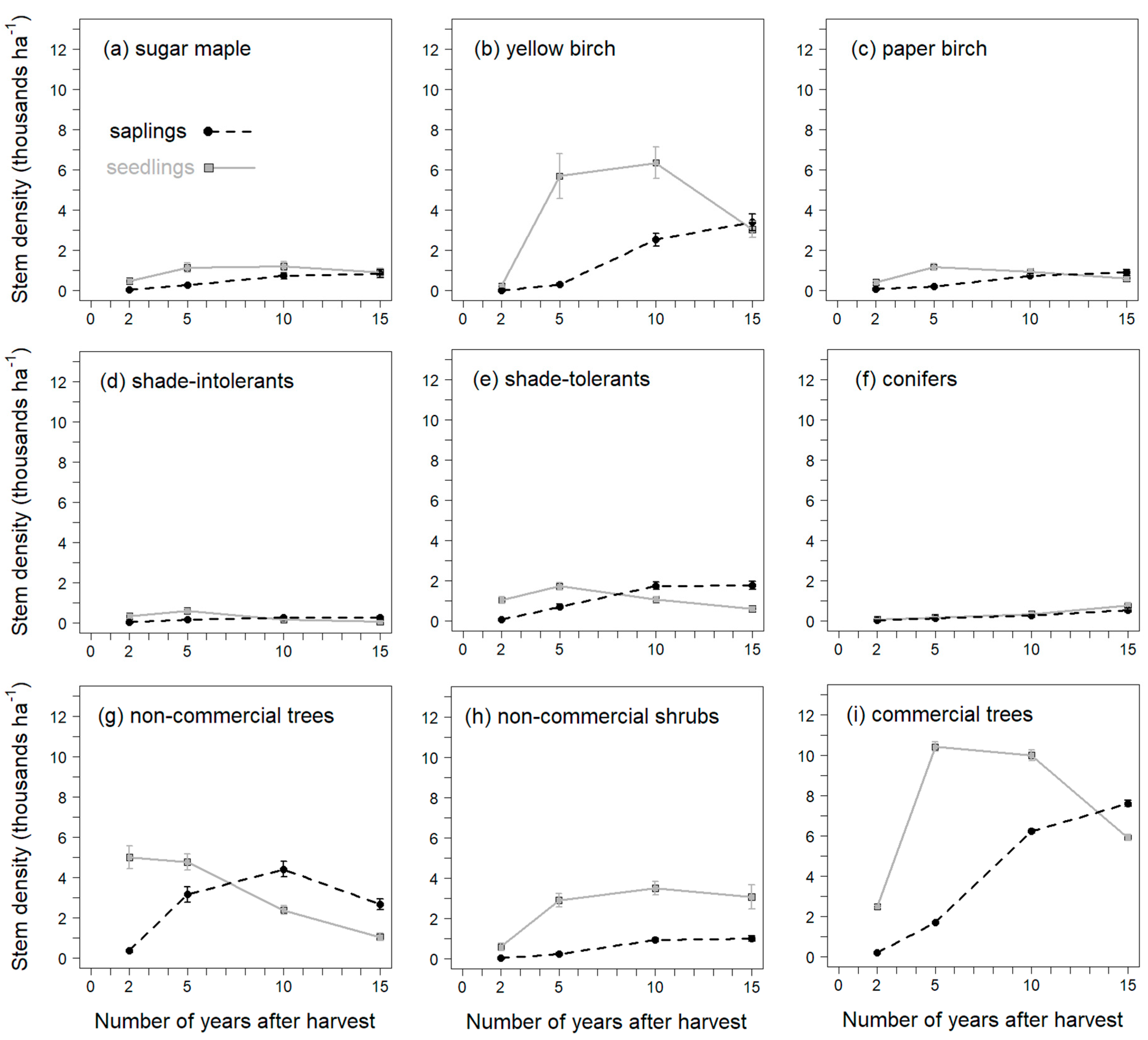A stocking of 40% obtained with sampling units of that size would mean that there is at least one commercial species located in 640 out of the 1600 possible sampling units per hectare (10,000 m² ÷ 6.25 m² = 1600), thus resulting in a tree density of at least 640 stems properly spaced per hectare. In addition, every cluster had a density of commercial species of at least 2500 stems ≥ 1 m in height ha⁻¹, well above the recommended stocking of 1500 stems ha⁻¹ from Leak et al. [34] (Figure 5a). When considering saplings only, all clusters had densities above the minimum stocking of 1000 stems ha⁻¹ (Figure 5b). As suggested by Elenitsky et al. 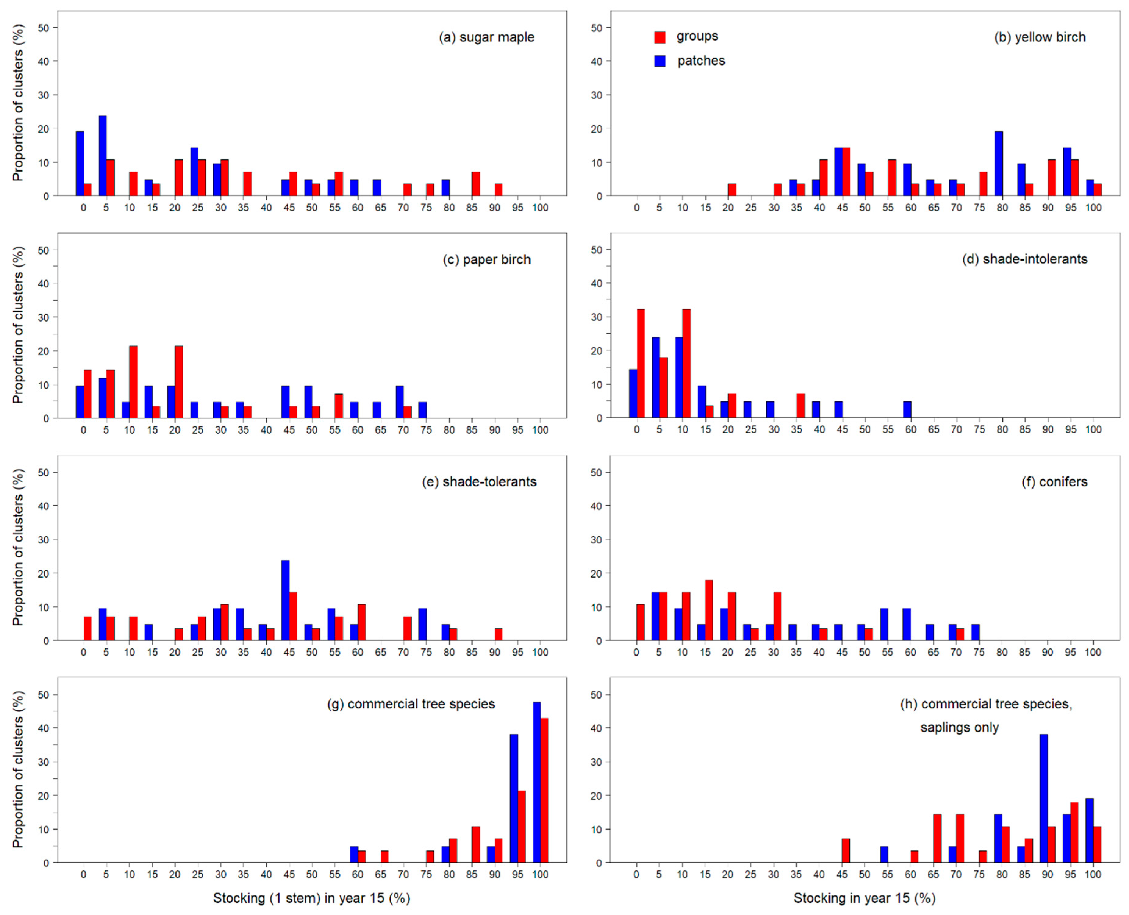[66], if we assume that (i) mortality is low as trees grow from saplings to 10-cm DBH, (ii) that saplings have transcended both deer browsing and shrub competition, and (iii) that a certain amount of seedlings ≥ 1 m in height will recruit into saplings in the near future, it would thus be sufficient to expect an eventual crown closure. Yellow birch, the main target species for natural regeneration and the most abundant commercial species in the current study, was present in all canopy openings, but with a highly variable distribution (mean Stock-1 = 62.5%, SD = 23, range = 15–100%, Figure 2b), as was also the case for sugar maple and the other commercial species pools (Figure 2a,c–f). Nevertheless, Stock-1 values for YB in all clusters were above the required thresholds from the Quebec management guidelines [26]. Additionally, mean densities of YB were always above the threshold of 1500 stems ha⁻¹ recommended by Leak et al. [34] for a successful regeneration (Figure 5a).

The fact that these canopy openings showed satisfyingly high mean densities, but sometimes had lower stocking of commercial species, especially saplings, indicate that those trees are abundant but not always so well distributed within openings. As a matter of fact, this has been observed elsewhere: in 9-year-old canopy openings created through group selection cutting, Poznanovic et al. [23] documented the spatial aggregation of YB, which they ascribed to spatial heterogeneity of suitable microsites. Six years later at these same sites, thus 15 years after harvest, Knapp et al. [67] observed that over half of the canopy openings they studied, ranging in size from 267 to 1192 m², harbored 10- to 310-m² portions of their area where regeneration, regardless of species, was no taller than 1.4 m. In comparison, they reported that 86% of saplings (all species combined) showed heights between 0.5 and 5 m. Hence, they concluded that their openings exhibited ‘spatially uneven patterns of regeneration, with areas of persistent and dense shrubs’ [67]. We observed this type of heterogeneity on the field in some of our canopy openings, often associated with a somewhat poorly drain soil, a very stony soil or intense cervid browsing, but these three hypotheses remain to be tested.

In our study, canopy openings created through harvest were of two very different sizes classes (1000 m² for groups vs. 15,000 m² for patches, on average). Yet, YB regeneration did not differ between the two size classes. Previous authors have similarly observed no effect of gap sizes on the regeneration success of YB [21,47,48,50,68] despite establishing experimental gradients of gap sizes varying in surface area from 260 to 1600 m², and especially in studies with favorable microsites to YB germination covering on average 50% of the area [21,47,48,68]—a scarification result similar to that at our sites, see Beaudet et al. [52]. Other studies nonetheless reported effects of gap size on YB regeneration success, although they used a gradient that reached down to very small sizes (<300 m²) and were located in stands where shade-tolerant species such as sugar maple and American beech were abundant [21,67,68,69,70] which was not often the case in this study. In addition, Bolton and D’Amato [21] as well as Shields et al. [68] acknowledged that the minimal soil disturbance that occurred in their gaps was not sufficient to create suitable germination microsites for YB. Incidentally, such factors (small gaps, abundance of shade-tolerants, and no soil scarification) are often reunited in studies where YB regeneration was the least successful, with relative stem densities of 5% or less [67,69,70].

The stem densities of yellow birch reached in our study are comparable to those of Shabaga et al. [71] in the neighboring Canadian province of Ontario. They reported after 10 years mean YB densities of 7000 stems ha⁻¹ for the ‘large regeneration’, which in their case comprised all individuals > 50 cm in height. Yet they observed large variation between ‘systematic gaps’ (≈5000 stems ha⁻¹) and ‘traditional gaps’ (≈14,000 stems ha⁻¹). By traditional gaps, they meant gaps placed where favorable microsites as well as mature seed trees could be found, in opposition to systematic gaps that would be located along a fixed grid. In the present study, canopy openings were systematically positioned within a stand, although there were always several seed trees present around an opening. In year 10, we observed mean YB densities of 8865 stems ha⁻¹ (6350 seedlings ≥ 1 m in height plus 2515 saplings; Figure 4b). Given the difference in how developmental stages were grouped between Shabaga et al.’s [71] study and ours, we consider our numbers to be quite on par with theirs.

However, much higher densities than the mean of the present study were reported by Bédard and DeBlois [47] and Gauthier et al. [48] in experimental canopy openings ranging from 15 to 35 m in diameter in Quebec. Gauthier et al. [48] reported over 12,000 large (≥ 1 m in height) YB seedlings ha⁻¹ 5 years after a harvest that occurred in 2005 (in comparison to 5680 YB seedlings ha⁻¹ in our study), while for SM in the same height class they observed densities > 20,000 ha⁻¹ (1130 ha⁻¹ in our study). Bédard and DeBlois [47] observed stem densities of YB ≥ 1 m ranging from ≈13,000 large seedlings ha⁻¹ in fenced deer-exclusion openings to ≈2000 ha⁻¹ in non-fenced openings 5 years after a harvest that took place in 2000. Although the mean YB density in year 5 across all our studied openings is lower than in the two aforementioned studies, we did observe such high YB densities in a few cases (data not shown). Soil scarification in these two experimental studies was synchronized with a good seed year, while our study covered all the years from 2000 to 2005. The lack of synchronization with a good seed year has been shown to potentially limit the efficacy of scarification to regenerate YB in an experimental study [72]. Nonetheless, we did not observe any obvious annual variation in YB regeneration in our study that could be explained by differences in seed years (data not shown). As a matter of fact, the receptivity of soil microsites to YB regeneration can reach up to 3 years [73]. Regarding relative abundance, both Gauthier et al. [48] and Bédard and DeBlois [47] reported values of 21% for YB in year 5. In comparison, our study sites presented in year 5 a mean %YB of 16% (SD = 13, range = 0.2 to 76%) for stems ≥ 1 m in height, which increased by year 15 to 27% (SD = 17, range = 4 to 73%).

The first regeneration survey, conducted in the second year after soil scarification, presented a situation where the non-commercial trees and shrubs dominated stem density (Figure 4). These are either shade-intolerant, pioneer species that develop rapidly after the disturbance created by harvesting operations, or alternatively are pre-established shade-tolerants able to take advantage of the new opening and enhanced light availability [74,75]. Given that these first surveys are aimed in part at identifying potential regeneration failures requiring immediate actions to address and correct the issue, the outlook may be gloomy when target species are few within a regrowth of weeds. Nyland et al. [75] indeed warned that a strong early occupation of regenerating sites by pin cherry (Prunus pensylvanica) could become problematic. They defined the threshold as three individuals over 1 m in height per 4 m² (their actual numbers were three pin cherry over 3 ft per milacre). This would correspond to 7500 stems ha⁻¹. At our study sites, mean densities of NCOM-tree reached 7900 stems ha⁻¹ in year 5 (Figure 4g) and quickly decreased afterwards. However, that species pool was not composed only of pin cherry but also of two other species, mountain maple and striped maple. These three species, respectively, represented on average 28%, 50%, and 22% of the NCOM-tree density (data not shown). Overall, given successional dynamics of tree species in temperate hardwood forests, combined to the short life expectancy of several pioneers, desirable hardwoods eventually overgrow their competitors unless dominance by non-commercial trees is very strong [32]. Previous authors have similarly reported that early presence of short-lived competitors such as Rubus spp. did not have lasting impact on YB development [71,76,77].

The slight decrease in vertical dominance of SM, YB, INTOL, and TOL between year-2 and year-5, concurrent with the increase in dominance of NCOM-tree and NCOM-shrub, likely reflects the growth dynamics of the latter species (Table 6). The fact that dominance by SM and TOL did not increase greatly between year 2 and year 15 might be due to them being established prior to harvest, as well as not being able to profit from the canopy opening as much as YB did. Indeed, in that regard, YB was the most successful of the hardwood species, becoming increasingly dominant as the years passed, to the point that by year 15 it was the most frequently dominant species (Table 6). Quite contrasting results were reported by Poznanovic et al. [70]: between years-2 and -9 after group selection harvest, YB went from being present in 14% of sampling units down to 12%. This meant that a certain number of subplots occupied by that species in year 2 had none in year 9. Therefore, in their case, the issue was not whether YB was dominant, but whether it was present, since it represented at best 5.5% of total sapling density, rather dominated by sugar maple [70]. Later studies at these sites suggested that soil scarification would have been needed to better promote mid-tolerant and intolerant hardwoods [67].

Height or developmental stage attained by a target species at a certain age may also prove a valuable parameter in assessing whether post-harvest regeneration was successful. For instance, some experimental studies have reported heights for successfully regenerated YB within canopy openings: between 2.45 and 7.0 m in year 10 [69], or mostly below 4.5 m in year 9 [70], or between 6.0 and 10.5 m in year 15 after harvest [78]. In the present study, the highest mean-per-cluster maximum height for YB in year 15 was 8.10 m, with a mean of 3.23 m across all clusters (SD = 1.74; Figure S3). In that regard, our study would not be among the most successful. As a matter of fact, YB was not very often the tallest individual within a quadrat (Figure 3b), even though dominance increased noticeably over time (Table 6). Indeed, hardwood seedlings dominated by competitors in early years may turn out to become dominant at a later point in stand development. For example, Marquis [40] had observed that some sites harvested using patch cutting in order to promote birches (yellow + paper) were overcrowded with pin cherry 3 years after harvest. However, returning at the same sites 47 years later, Leak [79] reported that birches composed 60% of the dominant trees in these patches.

4.2. Predicting Future Stand Composition

Although predicting the future stand composition remains challenging, our study showed that the later abundance of target species within post-harvest regenerating canopy openings can be approximated using some early basic inventory metrics. The better performance of the 6.25 m² quadrat over the 25 m² plot indicated that smaller plots, such as the more common 4 m² plots (or milacre), are better. In addition, the generally higher coefficients of correlation obtained with observations in year 5, instead of year 2, advocate waiting until year 5 to evaluate the regeneration success.

We first investigated whether the presence of a species in a dominant position in a quadrat in year 2 or 5 was a good indicator of the species that will dominate the quadrat in year 15. In the best case, 83% of the quadrats dominated by a non-commercial tree in year 15 were already dominated by this species pool in year 5. At the opposite, only 33% of the quadrats dominated by either YB or a conifer in year 15 were already in this situation in year 5. Yet, when a non-commercial tree dominated in year 5, there was only a 46% chance for it to still be dominant in year 15, whereas a quadrat dominated by a YB in year 5 would still be dominated by that species in year 15 in 69% of cases. Consequently, this analysis of dominance led us to a certain number of observations: (1) early dominance within a quadrat is not necessarily representative of later dominance within the same quadrat; (2) early surveys (year 2) do not help much in predicting which species will occupy the top of the future canopy within the quadrat; (3) however, the fact that target species are overgrown by competitors in early years does not preclude them becoming more prominent over time; (4) the non-commercial tree species that are highly abundant after a harvest and rapidly occupy the upper layer of the developing canopy, thus competing strongly against commercial hardwoods, see their dominant presence receding over time.

Northern hardwoods being mid- to late-successional species, it is normal to see a delay in their accession to canopy dominance, as previously showed by McClure et al. [80] in 44- to 48-year-old canopy openings. Yet, these authors observed that all canopy trees had established no later than 4 years after opening creation, although the exact moment of establishment varied per species. Indeed, they stated that 75% of canopy sugar maples had been advance regeneration whereas 79% of canopy yellow birches had germinated only after opening creation. Hence, early years may be crucial for regenerating openings, since future canopy trees need to at least be present even though they are not yet dominant. For instance, in a study assessing regeneration after strip cutting in Massachusetts, USA, Allison et al. (2003) observed that pin cherry (Prunus pensylvanica) had been the most abundant species to regenerate immediately after harvest. However, four decades later, it had almost disappeared, being replaced by, in decreasing order of abundance: red maple, paper birch, sugar maple, and black birch (Betula lenta, a mid-tolerant species like yellow birch [12]). This shows that a harvested site dominated in early years by non-commercial, competing woody species may nonetheless mostly comprise desirable species in later years. Our data suggest a similar phenomenon over a 15-year time period. Adequate silvicultural interventions, such as scarifying the soil, may accelerate the post-harvest succession.

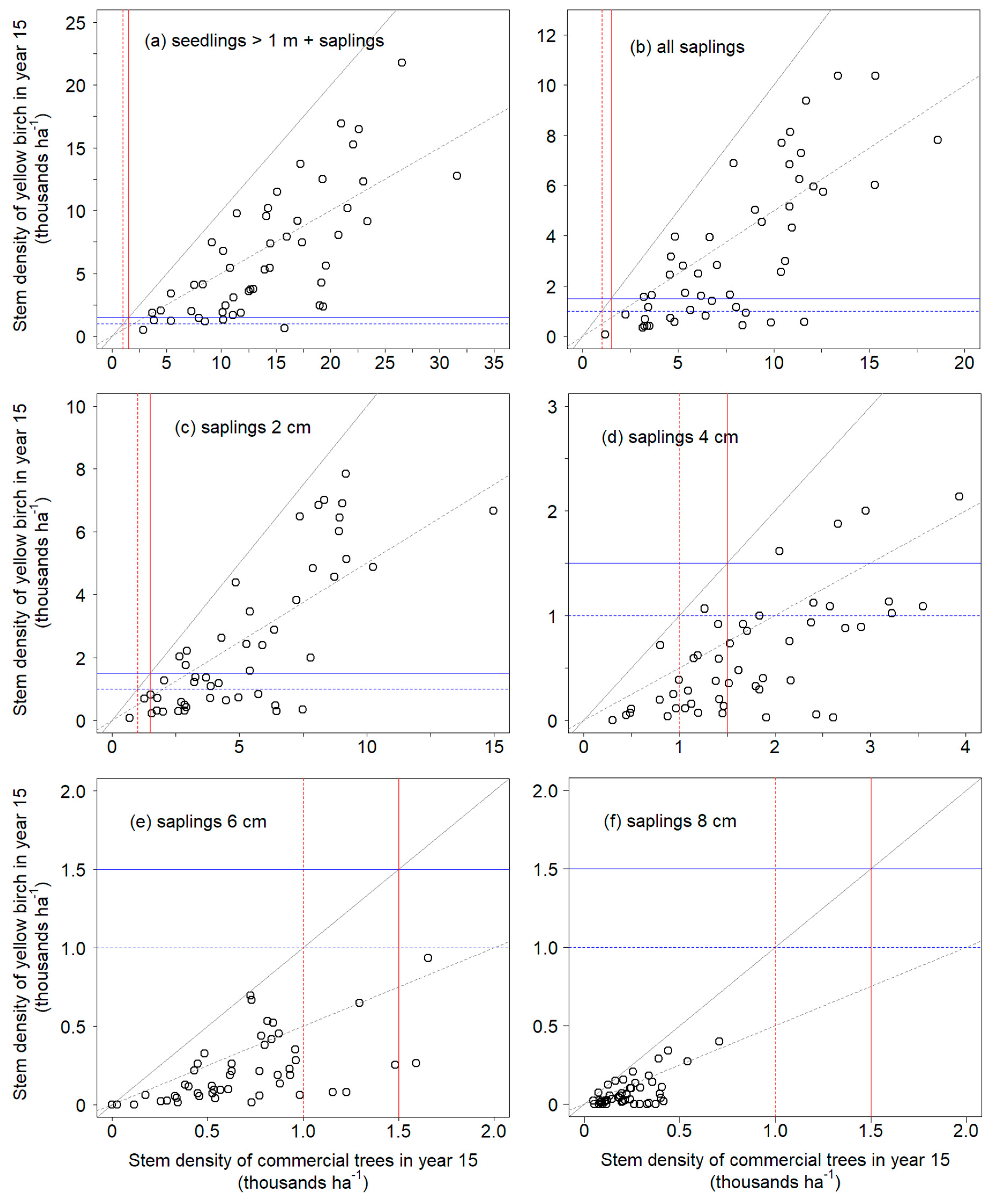
We identified some pertinent variables that could be measured in surveys conducted 5 years after the last treatment, either harvest or soil scarification, to better predict the composition relative abundance or relative basal area) in year 15. However, we did not delve into comparing how much time in the field must be dedicated to measuring each of these variables vs. their respective predictive power. The exact sets of variables differed slightly depending on the species under scrutiny, but %YB (or %SM) and Stock-1 in year 5 were always useful, except for Stock-1 in explaining %SM (Table 3 and Table 4). These variables indicate that abundant YB regeneration in year 15 can be obtained when it is well distributed within the opening and at a relatively high density among the stems at least 1 m in height. For example, if we would have created these openings with the aim of obtaining at least 50% of YB among all commercial species in year 15, it would have required the combination of a YB stocking between 20% and 100% with a relative abundance ranging from 35% to 80% (Equations (5) and (6)). More specifically, Equations (5) and (6) inform us that when Stock-1 ranges from 20% to 100% in year 5 (i.e., the value range observed at our sites for YB in that year), %YB in that same year must range from 50% to 35%, respectively, for the aforementioned Stock-1 values, in order to obtain 50% YB in BA or abundance in year 15. Only 16% of our clusters had a %YB in year 5 greater than 35% (with the highest value being 80%), and they concurrently had a Stock-1 between 71% and 100%. Obtaining a %YB above 50% in year 15 would thus require proportionally higher %YB in year 5, but could be achieved from a wide range of Stock-1 values. It demonstrates how %YB in stems ≥ 1 m in height was the most important indicator of future YB abundance. In the case of SM, the variables %SM, StD, Stock-1≥1m, and Stock-tallest in year 5 were identified as interesting predictors (Equations (9) and (10)). The models were more complex than for YB, but %SM of stems ≥ 1 m in height in year 5 was again the most important variable explaining variations in year 15 abundance. SM was less abundant within our canopy openings compared with YB, peaking at %SM values of 40% in year 5 and 60% in year 15 (Figure 7). Consequently, regeneration objectives would need to be adjusted: for instance, a %SM above 20% in year 15 would require year 5 variables in the order of 50% for Stock-1≥1m, 40% for Stock-tallest, and 20% for %SM.

In a paper comparing early post-harvest regeneration to stand composition ≈50 years later, Leak [37] reported that later relative basal area of pole-sized SM was best predicted by early relative number of SM saplings. This same measurement based on seedlings was not an accurate predictor of relative basal area of poles, because seedlings were so abundant in early years that they greatly overestimated later presence of SM poles. For YB, Leak [37] concluded that relative basal area after 50 years was most related to the early-year stocking based on the dominant (i.e., tallest) stem. In our study, we observed on the contrary that year-15 YB proportional presence was not related to Stock-tallest measured in year 2 or 5, but that this measure was appropriate for SM. These differences might be due to the differing types of harvest (Leak’s single-tree selection and diameter-limit cuttings vs. our group selection and patch cuttings) and the respective sizes of the resulting canopy openings.

5. Conclusions

Overall, our study showed that multi-cohort forest management that creates large or very large gaps in the canopy (respectively, group selection and patch cutting) can be generally successful in regenerating yellow birch, sugar maple, and other commercial tree species (Figure 5). However, the spatial distribution of the desired regeneration was not always homogeneous within openings, as revealed by some low coefficients of distribution (Figure 2). Densities of commercial stems at least 1 m in height were generally satisfying according to Leak et al.’s [34] recommendations. Even if considering yellow birch alone, a majority of clusters would have been deemed well stocked. However, if we were to limit the assessment to saplings, a number of clusters would have been understocked (Figure 5b–f).

In addition, our results indicated that the relative abundance of yellow birch was not very high, only 29% on average and never above ≈70% (Figure 6), even though these openings had been created for the purpose of regenerating this species in great numbers. Consequently, a cleaning treatment meant to eliminate trees of species that are not primary targets, undertaken not past the sapling stage [81], would be required in the future within most of these openings in order to increase the proportion of yellow birch. The non-commercial tree species that are highly abundant after a harvest may prove detrimental to early hardwood regeneration [74,75]. However, our results showed that they see their dominant presence receding over time, even though they remained important competitors (Table 6). Moreover, when non-commercial trees dominated a quadrat, the codominant was not often a YB (Figure 3d). Rather, when YB was the codominant, another commercial species often occupied the upper canopy (Figure 3b–e). This may suggest that the benefits of a cleaning could be lower than expected if it was aimed only at removing the non-commercial species without first assessing the situation on a per opening basis. Commercial species of secondary priority may thus need to be targeted as well during an eventual cleaning treatment in order to increase the relative presence and the dominance of YB within openings.

To verify the need for a cleaning treatment or to predict the future stand composition, regeneration surveys could be conducted 5 years after harvest using small sampling plots (6.25 m² in this study). The relative abundance (seedlings at least 1 m in height and saplings) in year 5 was the most important indicator of the relative abundance or basal area of either yellow birch or sugar maple in year 15, followed by the basic stocking (presence of one stem) in year 5 and, for sugar maple, some variants of it (one stem ≥ 1 m or the tallest stem). These should be decently good at predicting the relative presence of target species in the years to come. A cleaning treatment meant at increasing the relative abundance of the desired species could then be promising, especially when appropriately targeted at the most competing species and at the openings where desired hardwoods have a chance of becoming dominant afterwards.

References

1. Coates, K.D.; Burton, P.J. A gap-based approach for development of silvicultural systems to address ecosystem management objectives. For. Ecol. Manag. 1997, 99, 337–354. [Google Scholar] [CrossRef]
2. Hupperts, S.F.; Dickinson, Y.L.; Webster, C.R.; Kern, C.C. Promoting structural and species diversity in Great Lakes northern hardwoods: A conceptual model and its application. For. Int. J. For. Res. 2018, 92, 16–25. [Google Scholar] [CrossRef]
3. Puettmann, K.J.; Wilson, S.M.; Baker, S.C.; Donoso, P.J.; Drössler, L.; Amente, G.; Harvey, B.D.; Knoke, T.; Lu, Y.; Nocentini, S.; et al. Silvicultural alternatives to conventional even-aged forest management—What limits global adoption? For. Ecosyst. 2015, 2, 8. [Google Scholar] [CrossRef] [Green Version]
4. Mitchell, S.J. Wind as a natural disturbance agent in forests: A synthesis. For. Int. J. For. Res. 2012, 86, 147–157. [Google Scholar] [CrossRef] [Green Version]
5. Peterson, C.J.; Krueger, L.M.; Royo, A.A.; Stark, S.; Carson, W.P. Disturbance size and severity covary in small and mid-size wind disturbances in Pennsylvania northern hardwoods forests. For. Ecol. Manag. 2013, 302, 273–279. [Google Scholar] [CrossRef]
6. Runkle, J.R.; Yetter, T.C. Treefalls revisited: Gap dynamics in the southern appalachians. Ecology 1987, 68, 417–424. [Google Scholar] [CrossRef]
7. Canham, C.D. Growth and canopy architecture of shade-tolerant trees: Response to canopy gaps. Ecology 1988, 69, 786–795. [Google Scholar] [CrossRef]
8. Woods, K.D. Intermediate disturbance in a late-successional hemlock-northern hardwood forest. J. Ecol. 2004, 92, 464–476. [Google Scholar] [CrossRef]
9. Gasser, D.; Messier, C.; Beaudet, M.; Lechowicz, M.J. Sugar maple and yellow birch regeneration in response to canopy opening, liming and vegetation control in a temperate deciduous forest of Quebec. For. Ecol. Manag. 2010, 259, 2006–2014. [Google Scholar] [CrossRef] [Green Version]
10. Hanson, J.J.; Lorimer, C.G. Forest structure and light regimes following moderate wind storms: Implications for multi-cohort management. Ecol. Appl. 2007, 17, 1325–1340. [Google Scholar] [CrossRef]
11. Bannon, K.; Delagrange, S.; Bélanger, N.; Messier, C. American beech and sugar maple sapling relative abundance and growth are not modified by light availability following partial and total canopy disturbances. Can. J. For. Res. 2015, 45, 632–638. [Google Scholar] [CrossRef]
12. Burns, R.M.; Honkala, B.H. Silvics of North America: 2 Hardwoods; Department of Agriculture, Forest Service: Washington, DC, USA, 1990; Volume 2, p. 877. [Google Scholar]
13. Jones, T.A.; Domke, G.M.; Thomas, S.C. Canopy tree growth responses following selection harvest in seven species varying in shade tolerance. Can. J. For. Res. 2009, 39, 430–440. [Google Scholar] [CrossRef]
14. McClure, J.W.; Lee, T.D. Small-scale disturbance in a northern hardwoods forest: Effects on tree species abundance and distribution. Can. J. For. Res. 1993, 23, 1347–1360. [Google Scholar] [CrossRef]
15. Godman, R.M.; Yawney, H.W.; Tubbs, C.H. Acer Saccharum Marsh Sugar Maple. In Silvics of North America, 654th ed.; Burns, R.M., Honkala, B.H., Eds.; Department of Agriculture, Forest Service: Washington, DC, USA, 1990; Volume 2, pp. 78–91. [Google Scholar]
16. Nolet, P.; Delagrange, S.; Bouffard, D.; Doyon, F.; Forget, E. The successional status of sugar maple (Acer saccharum), revisited. Ann. For. Sci. 2008, 65, 1–10. [Google Scholar] [CrossRef] [Green Version]
17. Raymond, P.; Royo, A.A.; Prévost, M.; Dumais, D. Assessing the single-tree and small group selection cutting system as intermediate disturbance to promote regeneration and diversity in temperate mixedwood stands. For. Ecol. Manag. 2018, 430, 21–32. [Google Scholar] [CrossRef]
18. Reuling, L.F.; D’Amato, A.W.; Palik, B.J.; Martin, K.J.; Fassnacht, D.S.A. Initial tree regeneration response to natural-disturbance-based silviculture in second-growth northern hardwood forests. Can. J. For. Res. 2019, 49, 628–639. [Google Scholar] [CrossRef]
19. Webster, C.R.; Lorimer, C.G. Single-tree versus group selection in hemlock-hardwood forests: Are smaller openings less productive? Can. J. For. Res. 2002, 32, 591–604. [Google Scholar] [CrossRef]
20. Angers, V.A.; Messier, C.; Beaudet, M.; Leduc, A. Comparing composition and structure in old-growth and harvested (selection and diameter-limit cuts) northern hardwood stands in Quebec. For. Ecol. Manag. 2005, 217, 275–293. [Google Scholar] [CrossRef] [Green Version]
21. Bolton, N.W.; D’Amato, A.W. Regeneration responses to gap size and coarse woody debris within natural disturbance-based silvicultural systems in northeastern Minnesota, USA. For. Ecol. Manag. 2011, 262, 1215–1222. [Google Scholar] [CrossRef]
22. Webster, C.R.; Jensen, N.R. A shift in the gap dynamics of Betula alleghaniensis in response to single-tree selection. Can. J. For. Res. 2007, 37, 682–689. [Google Scholar] [CrossRef]
23. Poznanovic, S.K.; Poznanovic, A.J.; Webster, C.R.; Bump, J.K. Spatial patterning of underrepresented tree species in canopy gaps 9years after group selection cutting. For. Ecol. Manag. 2014, 331, 1–11. [Google Scholar] [CrossRef]
24. Raymond, P.; Bédard, S.; Roy, V.; Larouche, C.; Tremblay, S. The Irregular Shelterwood System: Review, Classification, and Potential Application to Forests Affected by Partial Disturbances. J. For. 2009, 107, 405–413. [Google Scholar]
25. Buda, N.J.; White, R.G. Forest Regeneration Standards in Ontario: A Historical Perspective; Ontario Ministry of Natural Resources, Northwest Science & Information: Thunder Bay, ON, Canada, 2007; pp. 1–24. [Google Scholar]
26. MRNFP. Manuel D’aménagement Forestier; Direction de la Planification et des Communications, Ministère des Ressources Naturelles, de la Faune et des Parcs, Gouvernement du Québec: Québec, QC, Canada, 2003; p. 245.
27. Brand, D.G.; Leckie, D.G.; Cloney, E.E. Forest regeneration surveys: Design, data collection, and analysis. For. Chron. 1991, 67, 649–657. [Google Scholar] [CrossRef] [Green Version]
28. Stein, W.I. Regeneration Surveys and Evaluation. In Reforestation Practices in Southwestern Oregon and Northern California; Hobbs, S.D., Ed.; Forest Research Laboratory, Oregon State University: Corvallis, OR, USA, 1992; Available online: https://ir.library.oregonstate.edu/downloads/3r074v462 (accessed on 7 July 2020).
29. Yang, Y.; Huang, S.; Dick Dempster, W.R. Percent stocking models for four major Alberta tree species. For. Int. J. For. Res. 2008, 81, 599–615. [Google Scholar] [CrossRef] [Green Version]
30. Bonham, C.D. Measurements for Terrestrial Vegetation, 2nd ed.; John Wiley & Sons, Ltd.: Hoboken, NJ, USA, 2013; p. 246. [Google Scholar] [CrossRef]
31. Raunkiær, C.C. The Life Forms of Plants and Statistical Plant Geography; Oxford University Press: Oxford, UK, 1934; p. 632. [Google Scholar]
32. Leak, W.B. Effects of Weed Species on Northern Hardwood Regeneration in New Hampshire. North. J. Appl. For. 1988, 5, 235–237. [Google Scholar] [CrossRef]
33. Hosie, R.C. Forest Regeneration in Ontario Based on a Review of Surveys Conducted in the Province during the Period 1918–1951; University of Toronto Press: Toronto, ON, Canada, 1953. [Google Scholar]
34. Leak, W.B.S.; Dale, S.; DeBald, P.S. Silvicultural Guide for Northern Harwood Types in the Northeast (Revised); Departement of Agriculture, Forest Service, Northeastern Forest Experimental Station: Broomall, PA, USA, 1987; p. 36.
35. Farnden, C. An analysis framework for linking regeneration standards to desired future forest conditions. For. Chron. 2009, 85, 285–292. [Google Scholar] [CrossRef] [Green Version]
36. Farnden, C. Observations on relationships between regeneration stocking and yield. For. Ecol. Manag. 2010, 260, 1507–1515. [Google Scholar] [CrossRef]
37. Leak, W.B. Accuracy of Regeneration Surveys in New England Northern Hardwoods. North. J. Appl. For. 2007, 24, 227–229. [Google Scholar] [CrossRef]
38. Halpin, C.R.; Lorimer, C.G.; Hanson, J.J.; Palik, B.J. Predicted long-term effects of group selection on species composition and stand structure in northern hardwood forests. For. Ecol. Manag. 2017, 400, 677–691. [Google Scholar] [CrossRef]
39. Leak, W.B.; Filip, S.M. Thirty-eight years of group selection in New England northern hardwoods. J. For. 1977, 75, 641–643. [Google Scholar]
40. Marquis, D.A. Regeneration of Birch and Associated Hardwoods after Patch Cutting; RP-NE-032; Department of Agriculture, Forest Service, Northeastern Forest Experiment Station: Upper Darby, PA, USA, 1965; p. 13.
41. Miller, G.W.; Wood, P.B.; Nichols, J.V. Two-Age Silviculture: An Innovative tool for Enhancing Species Diversity and Vertical Structure in Appalachian Hardwoods. In Forest Health through Silviculture: Proceedings of the 1995 National Silviculture Workshop; US Department of Agriculture, Forest Service, Rocky Mountain Forest and Range Experiment Station: Fort Collins, CO, USA, 1995. [Google Scholar]
42. Elie, J.-G.; Ruel, J.-C.; Lussier, J.-M. Effect of Browsing, Seedbed, and Competition on the Development of Yellow Birch Seedlings in High-Graded Stands. North. J. Appl. For. 2009, 26, 99–105. [Google Scholar] [CrossRef] [Green Version]
43. Erdmann, G.G. Betula alleghaniensis Britton Yellow Birch. In Silvics of North America, 654th ed.; Burns, R.M., Honkala, B.H., Eds.; U.S. Department of Agriculture, Forest Service: Washington, DC, USA, 1990; Volume 2. [Google Scholar]
44. Hatcher, R.J. Yellow birch regeneration on scarified seedbeds under small canopy openings. For. Chron. 1966, 42, 350–358. [Google Scholar] [CrossRef] [Green Version]
45. Linteau, A. Factors affecting germination and early survival of yellow birch (Betula lutea Michx) in Quebec. For. Chron. 1948, 24, 27–86. [Google Scholar] [CrossRef] [Green Version]
46. Marquis, D.A. Germination and Growth of Paper Birch and Yellow Birch in Simulated Strip Cuttings; U.S. Department of Agriculture, Forest Service, Northeastern Forest Experiment Station: Upper Darby, PA, USA, 1966; p. 19.
47. Bédard, S.; DeBlois, J. Effets de trouées sylvicoles sur l’établissement de la régénération d’une érablière à bouleau jaune après cinq ans. Forestière; Direction de la Recherche Forestière, Ed.; Ministère Ressources Naturelles: Quebec, QC, Canada, 2010; p. 28.
48. Gauthier, M.-M.; Lambert, M.-C.; Bédard, S. Effects of Harvest Gap Size, Soil Scarification, and Vegetation Control on Regeneration Dynamics in Sugar Maple-Yellow Birch Stands. For. Sci. 2016, 62, 237–246. [Google Scholar] [CrossRef] [Green Version]
49. Lorenzetti, F.; Delagrange, S.; Bouffard, D.; Nolet, P. Establishment, survivorship, and growth of yellow birch seedlings after site preparation treatments in large gaps. For. Ecol. Manag. 2008, 254, 350–361. [Google Scholar] [CrossRef]
50. Prévost, M.; Raymond, P.; Lussier, J.-M. Regeneration dynamics after patch cutting and scarification in yellow birch—Conifer stands. Can. J. For. Res. 2010, 40, 357–369. [Google Scholar] [CrossRef]
51. Régnière, J.; Saint-Amant, R. BioSIM 9: User’s Manual, Natural Resources Canada; C.F.S., Laurentian Forestry Centre: Québec, QC, Canada, 2008; pp. 1–68.
52. Beaudet, M.; Bédard, S.; Lambert, M.-C.; Hamel, J. Effets Réels Quinquennaux des Coupes de Jardinage par Trouées et des Coupes de Jardinage Avec Régénération par Parquets Pratiquées de 2000 à 2005 en Forêt Feuillue et Mixte; Gouvernement du Québec, Ministère des Ressources Naturelles, Direction de la Recherche Forestière: Québec, QC, Canada, 2014; p. 41.
53. Saucier, J.-P.; Berger, J.-P.; D’Avignon, H.; Racine, P. Le point d’observation écologique; Ministère des Ressources Naturelles, Directions des Stocks Forestiers, Service des Inventaires Forestiers: Québec, QC, Canada, 1994; p. 116.
54. Bashant, A.L.; Nyland, R.D.; Engelman, H.M.; Bohn, K.K.; Verostek, J.M.; Donoso, P.J.; Nissen, R.L., Jr. The Role of Interfering Plants in Regenerating Hardwood Stands of Northeastern North America; Maine Agricultural and Forest Experiment Station, The University of Maine: Orono, ME, USA, 2005; p. 66. [Google Scholar]
55. Donoso, P.J.; Nyland, R.D. Interference to Hardwood Regeneration in Northeastern North America: The Effects of Raspberries (Rubus spp.) Following Clearcutting and Shelterwood Methods. North. J. Appl. Forest. 2006, 23, 288–296. [Google Scholar] [CrossRef] [Green Version]
56. Haig, I.T. The Stocked-Quadrat Method of Sampling Reproduction Stands. J. For. 1931, 29, 747–749. [Google Scholar] [CrossRef]
57. Lowdermilk, W.C. A Method for Rapid Surveys of Vegetation. J. For. 1927, 25, 181–185. [Google Scholar] [CrossRef]
58. Bohn, K.K.; Nyland, R.D. Forecasting development of understory American beech after partial cutting in uneven-aged northern hardwood stands. For. Ecol. Manag. 2003, 180, 453–461. [Google Scholar] [CrossRef]
59. Bretz, F.; Posch, M.; Glimm, E.; Klinglmueller, F.; Maurer, W.; Rohmeyer, K. Graphical approaches for multiple comparison procedures using weighted Bonferroni, Simes, or parametric tests. Biom. J. 2011, 53, 894–913. [Google Scholar] [CrossRef] [PubMed] [Green Version]
60. Faraway, J.J. Extending the Linear Model with R: Generalized Linear, Mixed Effects and Nonparametric Regression Models; Chapman & Hall/CRC: Boca Raton, FL, USA, 2006; p. 331. [Google Scholar]
61. Strauss, D. The Many Faces of Logistic Regression. Am. Stat. 1992, 46, 321–327. [Google Scholar] [CrossRef]
62. Satterthwaite, F.E. An Approximate Distribution of Estimates of Variance Components. Biom. Bull. 1946, 2, 110–114. [Google Scholar] [CrossRef]
63. Burnham, K.P.; Anderson, D.R. Model Selection and Multimodel Inference: A Practical Information-Theoretic Approach, 2nd ed.; Springer: New York, NY, USA, 2002; p. 488. [Google Scholar]
64. Harrell, F.E., Jr. Package ‘Hmisc’, Version 4.3-0; CRAN: Toronto, ON, Canada, 2019; p. 424. [Google Scholar]
65. Bates, D.; Mächler, M.; Bolker, B.; Walker, S. Fitting Linear Mixed-Effects Models Using lme4. J. Stat. Softw. 2015, 67, 1–48. [Google Scholar] [CrossRef]
66. Elenitsky, L.M.; Walters, M.B.; Farinosi, E.J. Tree Regeneration Structure Following Beech Bark Disease-Motivated Harvests: Factors Associated with Patterns and Management Implications. Forests 2020, 11, 80. [Google Scholar] [CrossRef] [Green Version]
67. Knapp, S.P.; Webster, C.R.; Kern, C.C. Can group selection with legacy retention change compositional trajectories in conventionally managed hardwoods? For. Ecol. Manag. 2019, 448, 174–186. [Google Scholar] [CrossRef]
68. Shields, J.M.; Webster, C.R.; Nagel, L.M. Factors influencing tree species diversity and Betula alleghaniensis establishment in silvicultural openings. For. Int. J. For. Res. 2007, 80, 293–307. [Google Scholar] [CrossRef] [Green Version]
69. Kelty, M.J.; Nyland, R.D. Regenerating Adirondack Northern Hardwoods By Shelterwood Cutting and Control of Deer Density. J. For. 1981, 79, 22–26. [Google Scholar] [CrossRef]
70. Poznanovic, S.K.; Webster, C.R.; Bump, J.K. Maintaining mid-tolerant tree species with uneven-aged forest management: 9-year results from a novel group-selection experiment. For. Int. J. For. Res. 2013, 86, 555–567. [Google Scholar] [CrossRef] [Green Version]
71. Shabaga, J.A.; Jones, T.A.; Elliott, K.A. Group-selection silviculture conditionally enhances recruitment of yellow birch in a shade-tolerant hardwood forest. For. Ecol. Manag. 2019, 444, 244–255. [Google Scholar] [CrossRef]
72. Raymond, P.; Prévost, M.; Roy, V. Silvicultural options for rehabilitating high-graded mixedwood stands in northeastern North America. For. Ecol. Manag. 2020, 466, 118137. [Google Scholar] [CrossRef]
73. Gastaldello, P.; Ruel, J.-C.; Lussier, J.-M. Remise en production des bétulaies jaunes résineuses dégradées: Étude du succès d’installation de la régénération. For. Chron. 2007, 83, 742–753. [Google Scholar] [CrossRef] [Green Version]
74. Nyland, R.D.; Bashant, A.L.; Bohn, K.K.; Verostek, J.M. Interference to Hardwood Regeneration in Northeastern North America: Ecological Characteristics of American Beech, Striped Maple, and Hobblebush. North. J. Appl. For. 2006, 23, 53–61. [Google Scholar] [CrossRef] [Green Version]
75. Nyland, R.D.; Bashant, A.L.; Heitzman, E.F.; Verostek, J.M. Interference to Hardwood Regeneration in Northeastern North America: Pin Cherry and Its Effects. North. J. Appl. For. 2007, 24, 52–60. [Google Scholar] [CrossRef] [Green Version]
76. Kern, C.C.; Reich, P.B.; Montgomery, R.A.; Strong, T.F. Do deer and shrubs override canopy gap size effects on growth and survival of yellow birch, northern red oak, eastern white pine, and eastern hemlock seedlings? For. Ecol. Manag. 2012, 267, 134–143. [Google Scholar] [CrossRef]
77. Widen, M.J.; Petras O’Neil, M.A.; Dickinson, Y.L.; Webster, C.R. Rubus persistence within silvicultural openings and its impact on regeneration: The influence of opening size and advance regeneration. For. Ecol. Manag. 2018, 427, 162–168. [Google Scholar] [CrossRef]
78. Webster, C.R.; Lorimer, C.G. Minimum opening sizes for canopy recruitment of midtolerant tree species: A retrospective approach. Ecol. Appl. 2005, 15, 1245–1262. [Google Scholar] [CrossRef]
79. Leak, W.B. Regeneration of patch harvests in even-aged northern hardwoods in New England. North. J. Appl. For. 2003, 20, 188–189. [Google Scholar]
80. McClure, J.; Lee, T.; Leak, W. Gap capture in northern hardwoods: Patterns of establishment and height growth in four species. For. Ecol. Manag. 2000, 127, 181–189. [Google Scholar] [CrossRef]
81. Heitzman, E.; Nyland, R.D. Cleaning and early crop-tree release in northern hardwood stands: A review. North. J. Appl. For. 1991, 8, 111–115. [Google Scholar] [CrossRef]
Figure 1. Location of study sites within the province of Quebec, Canada.
Forests 11 00742 g001
Figure 2. Regeneration stockings, calculated on 6.25-m2 quadrats and considering all seedlings and saplings, for commercial tree species within canopy openings (groups, red, or patches, blue) 15 years after harvest. Data are cluster means, shown separately (ah) per species or species pool (see Table 1). Units on the x-axis represent the upper end of classes of five points of percentage, i.e., 100 is ]95–100], 95 is ]90–95], etc., but 0 is only 0.
Forests 11 00742 g002
Figure 3. Regeneration stockings for yellow birch (YB), calculated on 6.25-m2 quadrats and considering all seedlings and saplings, within canopy openings 15 years after harvest. Bars represent the proportion of clusters that show a given 5%-class of stocking. Points are mean sapling densities (all DBH classes) of YB per stocking class. Both stocking and density data are cluster means. Stocking was computed in five different ways: (a) based on a single YB stem per quadrat, (b) based on YB being the tallest stem in the quadrat, (c) based on YB being the second tallest stem in the quadrat regardless of the identity of the tallest stem, (d) based on YB being the second tallest stem when a non-commercial tree (NCOM-tree) was the tallest, and (e) based on YB being either the tallest stem or the second tallest when NCOM-tree was the tallest, thus a combination of (b,d). Horizontal solid and dashed lines represent, respectively, the 1500 and 1000 stems ha−1 density thresholds proposed by Leak et al. 1987 to assess post-harvest regeneration success.
Forests 11 00742 g003
Figure 4. Stem density over time, per developmental stage (seedlings ≥ 1 m in height, saplings) and per species or species pool (see Table 1). Data are cluster means (groups and patches combined) averaged per year and per species or species pool (ai). Error bars are standard errors.
Forests 11 00742 g004
Figure 5. Relationship between stem density of yellow birch and stem density of all commercial tree species 15 years after harvest within canopy openings created by group selection and patch cutting. Data points are cluster means, presented for different developmental stages: (a) seedlings at least 1 m in height and saplings, (b) all saplings, and (cf) saplings further distinguished by their diameter at breast height (DBH, in cm). Note the change in scales. Solid grey line is the 1:1 relationship and dashed grey line is the 1:0.5 relationship. Blue horizontal and red vertical lines represent the 1000 (dashed) and 1500 (solid) stems ha−1 thresholds based on Leak et al. 1987.
Forests 11 00742 g005
Figure 6. Relationships between relative abundance of yellow birch in year 15 and four different regeneration indices in year 2 (a,c,e,g) and year 5 (b,d,f,h), measured at the scale of 6.25-m2 quadrats. Stockings were computed on all seedlings and saplings, while stem densities were computed on seedlings ≥ 1 m in height and saplings. Data points are cluster means. Red dots are groups, blue dots are patches. Adjusted R2 and p-values were computed from simple linear regressions.
Forests 11 00742 g006
Figure 7. Relationships between relative abundance of sugar maple in year 15 and four different regeneration indices in year 2 (a,c,e,g) and year 5 (b,d,f,h), measured at the scale of 6.25-m2 quadrats. Stockings were computed on all seedlings and saplings, while stem densities were computed on seedlings ≥ 1 m in height and saplings. Data points are cluster means. Red dots are groups, blue dots are patches. Adjusted R2 and p-values were computed from simple linear regressions.
Forests 11 00742 g007
Figure 8. Mosaic plot of the evolution of dominance per quadrat (a) between year 2 and year 15 or (b) between year 5 and year 15. Levels of the two variables are individual species or species pool. Each cell of the contingency table is represented by a box. A box’s area is the total count in that cell, i.e., the number of quadrats where a given species was dominant in year 2 or 5 (rows) compared with which species was dominant in that same quadrat in year 15 (columns). Box width is the same for all boxes in a column and corresponds to the total count of that column. Box height is the proportion of quadrats in the column that fall into that cell. Blue-colored boxes indicate that there were more quadrats than expected under the null hypothesis (positive residuals), whereas red-colored boxes identify cells where there were fewer quadrats than expected (negative residuals). Standardized residuals were computed as the residual (i.e., observed minus expected value) divided by the square root of the expected value. Residuals above 2 or below −2 indicate significance at the 0.05 level.
Forests 11 00742 g008