Article

Estimating Mangrove Above-Ground Biomass Loss Due to Deforestation in Malaysian Northern Borneo between 2000 and 2015 Using SRTM and Landsat Images

1
Faculty of Science and Natural Resources, Universiti Malaysia Sabah, Kota Kinabalu 88400, Sabah, Malaysia
2
Sabah Forestry Department, Locked Bag 68, Sandakan 90009, Sabah, Malaysia
3
Graduate School of Agriculture and Life Science, The University of Tokyo, Yayoi 1-1-1, Bunkyo-Ku, Tokyo 113-0032, Japan
*
Author to whom correspondence should be addressed.
Forests 2020, 11(9), 1018; https://doi.org/10.3390/f11091018
Submission received: 30 July 2020 / Revised: 25 August 2020 / Accepted: 26 August 2020 / Published: 22 September 2020

Abstract

:
Mangrove forests are highly productive ecosystems and play an important role in the global carbon cycle. We used Shuttle Radar Topography Mission (SRTM) elevation data to estimate mangrove above-ground biomass (AGB) in Sabah, Malaysian northern Borneo. We developed a tree-level approach to deal with the substantial temporal discrepancy between the SRTM data and the mangrove’s field measurements. We predicted the annual growth of diameter at breast height and adjusted the field measurements to the SRTM data acquisition year to estimate the field AGB. A canopy height model (CHM) was derived by correcting the SRTM data with ground elevation. Regression analyses between the estimated AGB and SRTM CHM produced an estimation model (R2: 0.61) with a root mean square error (RMSE) of 8.24 Mg ha−1 (RMSE%: 5.47). We then quantified the mangrove forest loss based on supervised classification of multitemporal Landsat images. More than 25,000 ha of mangrove forest had disappeared between 2000 and 2015. This has resulted in a significant decrease of about 3.96 million Mg of mangrove AGB in Sabah during the study period. As SRTM elevation data has a near-global coverage, this approach can be used to map the historical AGB of mangroves, especially in Southeast Asia, to promote mangrove carbon stock conservation.

1. Introduction

Globally, deforestation and forest degradation have resulted in a substantial release of greenhouse gases (GHGs) to the atmosphere, constituting approximately 10% of global emissions [1]. The Reducing Emissions from Deforestation and Forest Degradation (REDD+) program has been negotiated under the United Nations Framework Convention on Climate Change (UNFCCC) as a viable option for reducing greenhouse-gas emissions from the land-use sector [2]. REDD+ provides financial incentives to assist in the reduction of national carbon emission rates due to deforestation and forest degradation in developing countries [3,4]. While most of the nations have focused on inland forest ecosystems especially tropical forests, the role of mangroves in climate change mitigation has gained considerable interest in recent years [5].
Mangrove forest is one of the most productive forest ecosystems in terms of its efficiency of carbon cycling and storage, as well as carbon sequestering [6,7,8]. Mangrove forests store five times more carbon per unit area than other forest ecosystems [7], and can store up to three times more carbon per unit area than other tropical forests [9,10]. However, increasing demand for mangrove products, such as materials for buildings and fuel, as well as urbanization, has led to the destruction and degradation of mangrove forests throughout the world [11]. Almost 20% of the world’s mangrove areas disappeared between 1980 and 2005 [12]. Recently, the global mangrove loss rate has been estimated to range between 0.16% and 0.39% annually [13]. The deforestation of mangroves causes the release of large amounts of carbon emissions into the atmosphere [14]. Mangrove forest is one of the three natural forest classes to be monitored for REDD in Malaysia [15]. About 58.6% of the nation’s mangrove forests are found in Sabah [16], making this state particularly important in the REDD implementation. The state’s mangrove forest was estimated at 327,678 ha around early 2000s [17], but changes since then are not known.
In order to better understand carbon emissions and the ecosystem structure of mangroves, we need to accurately quantify the ecosystem biomass, extent and change of mangroves by measuring their horizontal and vertical heterogeneity. Horizontal heterogeneity refers to the aspect of land cover and its change, whereas vertical heterogeneity is considered in terms of forest height, which is one of the main determinants of its above-ground biomass (AGB) [18]. Forest cover loss due to land use change can be monitored using multitemporal land-cover change analyses (e.g., [19,20]). For mangrove’s AGB or carbon stock estimations, only very few comprehensive assessments of mangrove’s carbon inventory have been performed to date [9,21]. Field measurements are the most accurate method for estimating AGB. However, it is expensive, time consuming and difficult to apply to a large area for mangroves, which often grow in an inter-tidal zone that is extremely difficult to access. Not only overcoming the problem of accessibility, remote sensing coupling with field measurements is a recommended AGB estimation approach for REDD+ [22].
Remote sensing has been used to retrieve forest structure and AGB information using large-spatial scale satellite images over a long-term basis and at a much lower cost [11]. Active remote sensing systems, such as synthetic aperture radar (SAR) and airborne light detection and ranging (LiDAR), can penetrate the forest canopy at different depths. These systems are relatively sensitive to forest component arrangements and can be used to estimate forest structures such as height [23]. SAR has limited success in estimating AGB, especially for tropical forests with high AGB [24]. Airborne LiDAR is accurate [25,26] but too expensive to use for a large-area survey. The Shuttle Radar Topography Mission (SRTM) mission, implemented in 2000, offers free and high-resolution (1-arc second or 30 m) digital elevation data that cover 80% of the Earth’s land surface between 56° S and 60° N. However, the C band radar signal that scatters with all forest components may not reach the ground. The SRTM data correlates well with the canopy heights of mangrove forests [27,28]. Therefore, the SRTM data is, in effect, a digital surface model (DSM). Assuming a flat coastal topography, SRTM DSM has been used to estimate AGB of mangroves in the Everglades National Park [29], Colombia [30], Mozambique [31], Africa [27], the French Guiana [32] and Indonesia’s Papua province [33]. Mangrove carbon stock was recently analyzed at a global scale using a combination of SRTM DEM, ICEsat/GLAS and field data [34]. The main sources of regression residuals between the remotely sensed height values and field height measurement or AGB include the timing of measurements, discrepancies in the spatial scale and several additional sources of uncertainty [27,30,31,34]. However, none of these studies has dealt with the large discrepancy between the dates of field measurement and the SRTM data acquisition.
In this study, we examined the estimation of mangrove AGB in Sabah, Malaysia using SRTM DSM with and without ground elevation correction. We addressed the time gap between the SRTM and field data by developing a tree-level diameter at breast height (DBH) prediction model to adjust the DBH measurements to the SRTM data acquisition year and estimated the field AGB. We quantified the mangrove AGB loss in Sabah between 2000 and 2015 using Landsat images and the predicted mangrove AGB map of 2000.

2. Materials and Methods

2.1. Study Area

Sabah, located in the northern part of Borneo Island, is the second-largest state of Malaysia (73,904 km2) (Figure 1). It has an annual mean temperature of 27 °C and an annual mean rainfall of 2788 mm. Sabah has a long coastline of about 4328 km, mainly covered by mangrove forests, many of which are legally gazetted as ‘Class I Protection Forest Reserve, Class V Mangrove Forest Reserves or Class VI Amenity Forest Reserve’ under the Sabah Forest Enactment (1968) [17]. Including water bodies, the total area of these reserves was about 340,000 ha in 2015 [35].

2.2. Field Inventory and AGB Data

Field measurements of mangrove forests focused on the West Coast of Sabah. Twenty-eight square plots (20 m × 20 m) were randomly sampled in 2018. We measured the diameter at breast height (DBH) and height (H) of trees larger than 5 cm DBH using a DBH tape and the TruPulse 360 Laser Rangefinder (Laser Technology Inc., Centennial, CO, USA), respectively. Measuring the height of mangrove trees inside the forest is difficult. We took three measurements from different directions and averaged them to obtain the height value. The plot coordinates were determined by a Differential Global Navigation Satellite System (GNSS) (JAVAD GNSS Triumph-1) (JAVAD GNSS Inc., San Jose, CA, USA). In addition, we obtained forty-two plots (10 m × 10 m) that were established using a transect line method in 2016 from another research project. We used the first and last plots in a transect line if the plots are separated more than 3 pixels or 90 m apart. Otherwise, plots from the same transect were averaged and treated as a single plot. Two of the 2016 plots that overlapped with the 2018 plots were excluded. In total, forty plots were available to this study for calculate field AGB. While both DBH and H were measured for the 2018 plots, these were measured in eighteen out of the 2016 plots. Only DBH was measured in the remaining plots. The plot locations were recorded using a handheld GNSS receiver (GARMIN GPSMAP 60 CSx) (Garmin Ltd., Olathe, KS, USA), averaged for two hours (up to 5 m horizontal accuracy). These field plots covered a distance of 235 km in the West Coast of Sabah in four districts i.e., Tuaran, Kota Marudu, Kota Belud and Kudat districts (Figure 1).
Overall, 3222 trees were measured in these forty plots. The dominant mangrove species were Rhizophora apiculata and Avicennia alba. Nonetheless, species information was only collected for some plots. AGB is generally predicted by DBH and/or height in an allometry and can be improved by including wood density information [36]. Without complete species information, the choice of AGB allometry was limited in this study. We used the allometric equation of Saenger and Snedaker [15] because it is a global stand height-AGB allometric equation that was calculated using 43 field data sets distributed globally. It has been widely applied with the SRTM data to estimate mangrove AGB (e.g., [28,29,30,31,34]) (Equation (2)).
AGB = 10.8 H + 34.9
where AGB is the above-ground biomass in Mg ha−1 and H is the tree height in meters. Equation (2) was used to estimate the field AGB in 2000. The field AGB 2000 was regressed against variables derived from the SRTM data in a least-squares regression analysis to develop an AGB estimation model for the mangroves of Sabah.
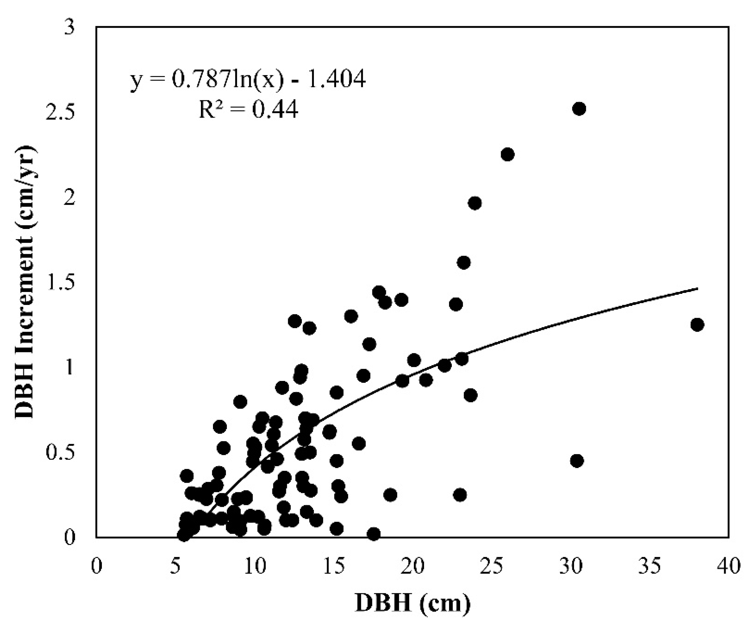
Since the SRTM data was acquired in year 2000, and the field data were collected in 2016 and 2018, we adjusted the tree measurements to year 2000 for their intermediate growth by using the method proposed by Clark et al. [37]. We collected two additional plots of DBH data measured in 2004 and 2006 by the Sabah Forestry Department. This data was used together with our DBH data from 2016 and 2018 to derive a model for relating annual DBH increase and DBH at tree level for mangroves of Sabah (Table 1 and Figure 2). DBH value of each tree was iteratively adjusted using the following model:
D B H y e a r 1 = D B H y e a r [ 0.787   × ln ( D B H y e a r ) 1.404 ]
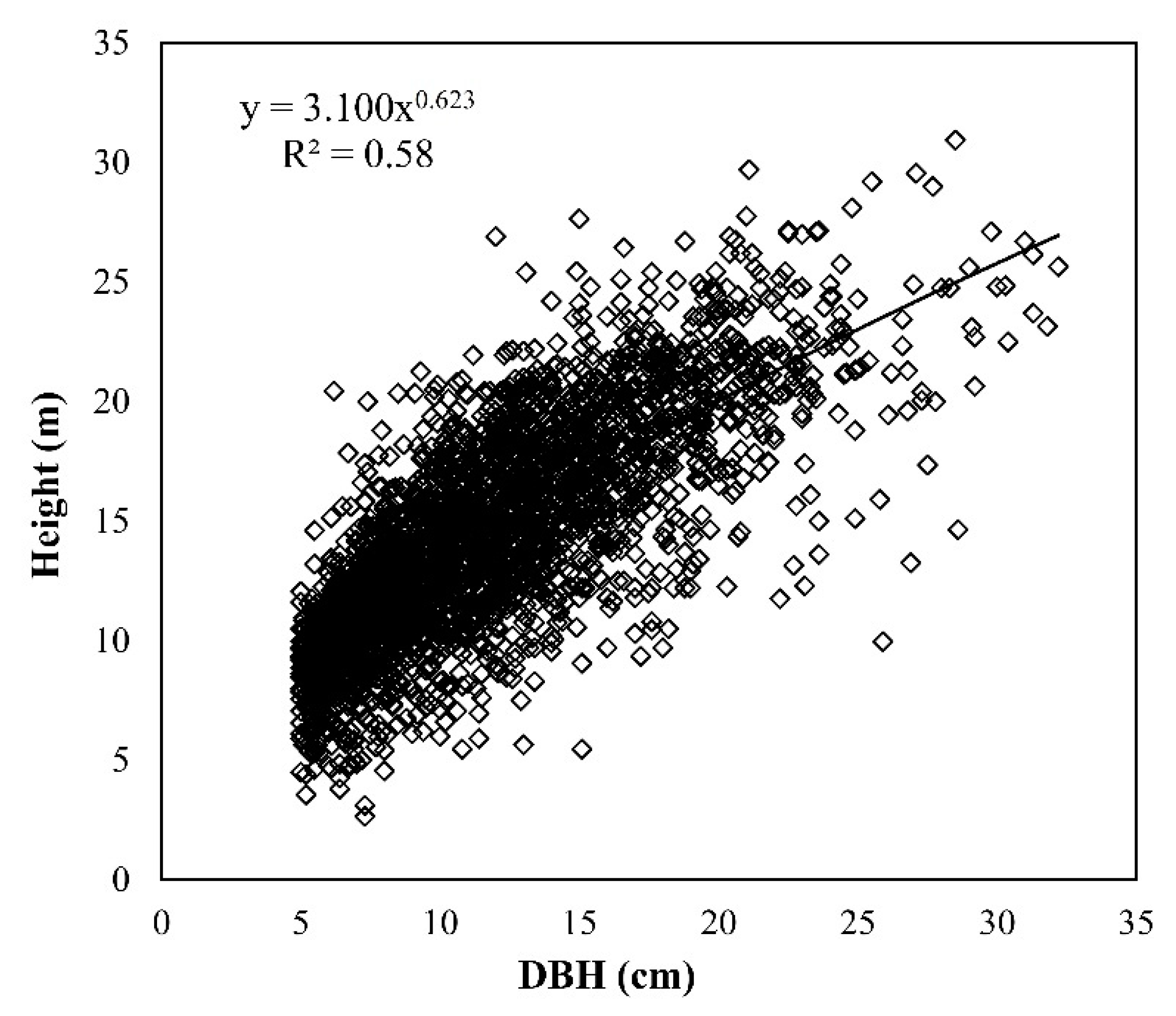
where DBHyear is the DBH of the actual measurement year and DBHyear−1 is the DBH of the previous year in cm. The DBH values were adjusted from the year in which it was measured until 2000, when the SRTM data was acquired. With the adjusted DBH values, we then estimated the tree height by establishing a DBH-height relationship based on mangrove trees that had both DBH and height measurements. Table 2 and Figure 3 show the regression between DBH and height for the mangrove trees, which had a coefficient of determination of 0.58 (n = 2760).

2.3. Land Cover Classification of Multi-Temporal Landsat Images

A supervised classification approach was used to map the mangrove forests of Sabah in years 2000 and 2015. The coastlines of Sabah are covered by eight Landsat scenes (Scene’s path/row no: 116/56; 116/57; 117/55; 117/56; 117/57; 118/55; 118/56; 118/57). However, we had to download more than thirty images from the United States Geological Survey website [38] for the same year to identify additional images with low cloud cover. For each scene, cloud-covered pixels in the best-quality image were masked out and filled with pixel values of other images within the same year. This was followed by converting the pixel’s digital numbers to top-of-atmosphere reflectance and atmospheric correction, using the dark object subtraction method. Supervised classification was conducted using the maximum likelihood algorithm, which classifies each pixel to a land cover class based on the class’s probability. Training areas for the classification were randomly collected on the high-resolution images in Google Earth and also with the help of a handheld Global Navigation Satellite System receiver during the field works. The classification resulted in seven land cover classes (water, mangrove, forest, plantation, agriculture, grassland and bare land). These classes were grouped to mangrove and non-mangrove to assess the classification accuracy in the error matrix and reported as percentage of correctness. The accuracy measures included the producer’s accuracy, user’s accuracy, overall accuracy and the kappa coefficient. The mangrove areas were extracted from the land cover classifications for further analysis of AGB changes.

2.4. Canopy Height Models from the SRTM Data

A total of 13 tiles of SRTM DSM (30 m resolution) that cover the entire state of Sabah were downloaded from the USGS website [39] and merged to form a raster mosaic. The SRTM DSM of the mangroves was extracted using the mangrove cover from the land cover classification 2000. These SRTM DSM values were used as a canopy height model for the coastal mangroves (CHMmg), because the topographic elevation values right below the mangrove forests are very close to the sea level and the radar height estimate is roughly the canopy height of mangroves [29,31]. We then examined whether correction of the CHM with a simulated digital terrain model (DTM) can improve the AGB estimation model for mangroves. The corrected CHM for mangroves (Corrected CHMmg) was derived as follows:
C o r r e c t e d   C H M m g = S R T M   D S M m g D T M m g
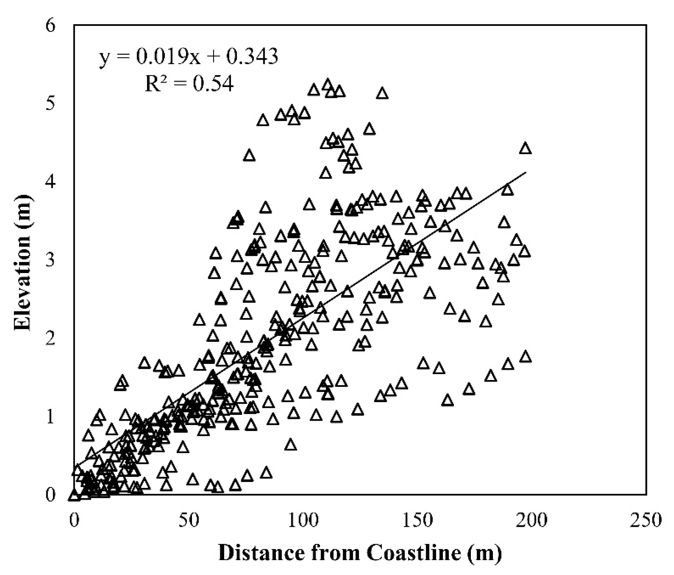
As the elevation of coastal areas typically increases from the coastline towards inland areas, the DTMmg was generated by establishing the relationship between distance from the coastline and elevation above mean sea level (Table 3 and Figure 4). The linear regression model thus derived was based on six coastal profiles obtained from the Sabah Shoreline Management Plan [40] as follows:
D T M m g = 0.019 D + 0.343
where DTMmg is the ground elevation in meters a.s.l. for mangrove cover and D is the distance from coastline in meters. D was generated as a raster (30 m × 30 m) by calculating the Euclidian distance from the Sabah coastline vector. We only generated the DTMmg for pixels less than 200 m from the coastline based on the coastal profiles. Beyond 200 m from the coastline, the SRTM DSM values were subtracted with the maximum value of DTMmg i.e., 4.1627 m based on Equation (4).

2.5. AGB Prediction Models

We extracted the pixel values from both CHMmg and Corrected CHMmg and calculated the average for each plot. The estimated field AGB was linearly regressed against the CHMmg and Corrected CHMmg. Natural-log transformation was also applied to the independent or dependent variable because height is known to have nonlinear relationship with AGB [41,42]. The best estimation models were selected based on R-Squared (R2), the root mean square error (RMSE) and the relative RMSE (RMSE%). RMSE was calculated with leave-one-out cross-validation to avoid overfitting of the model.

3. Results

3.1. Mangrove Forest Distribution

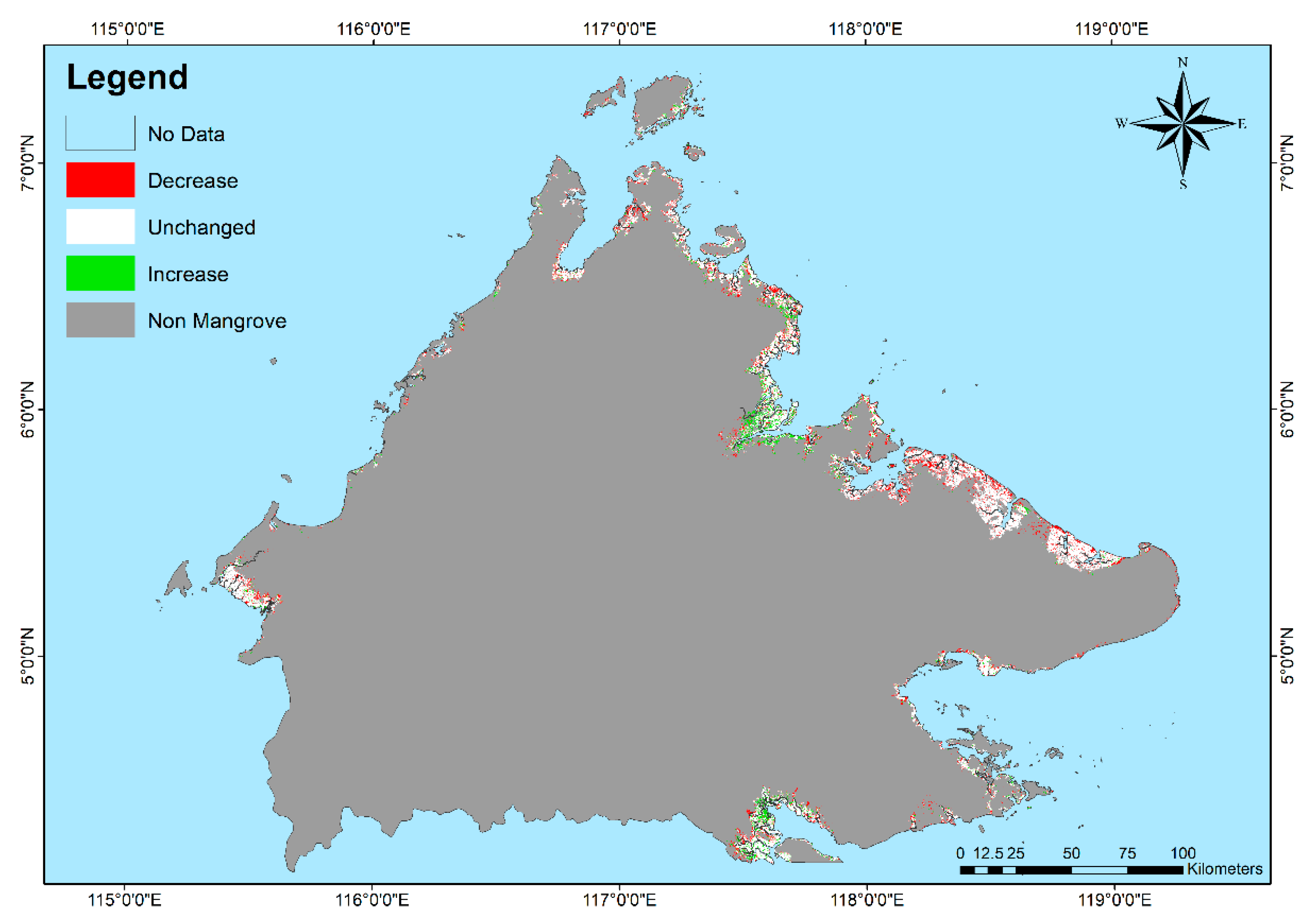
The land cover classification had an overall accuracy of 96.98% and 93.92% with kappa coefficients of 0.94 and 0.87 for years 2000 and 2015, respectively (Table 4). Reference data was obtained from Google Earth historical images to compare with the classified land cover classes (331 points for year 2000 and 329 points for year 2015). The overall mangrove area based on both classifications (2000 and 2015) generated mangrove areas of 294,207.75 ha and 268,631.91 ha, respectively. The changes of mangrove areas in Sabah were determined by subtracting the classified mangrove areas of 2000 and 2015. Figure 5 shows the increase, decrease and unchanged mangrove areas between 2000 and 2015. Although 58,262.85 ha of mangrove had disappeared, there was an increase of the forest cover of 32,687.01 ha in that fifteen years. About 235,944.9 ha of mangrove area remained unchanged.

3.2. AGB Estimation

Table 5 shows the descriptive statistics of the field measurements of mangrove forest variables at plot-level and their estimated values in year 2000. The field measurements had average DBH and height of 11.89 cm and 14.30 m, respectively. Estimation of the mangrove forest variables using the adjustment approach produced average DBH and height of 7.08 cm and 10.45 m, respectively. The AGB of individual trees within the plot was aggregated to generate the plot-level AGB (Mg ha−1). The measured field AGB had an average of 196.88 Mg ha−1, whereas the estimated field AGB in 2000 was 150.63 Mg ha−1.
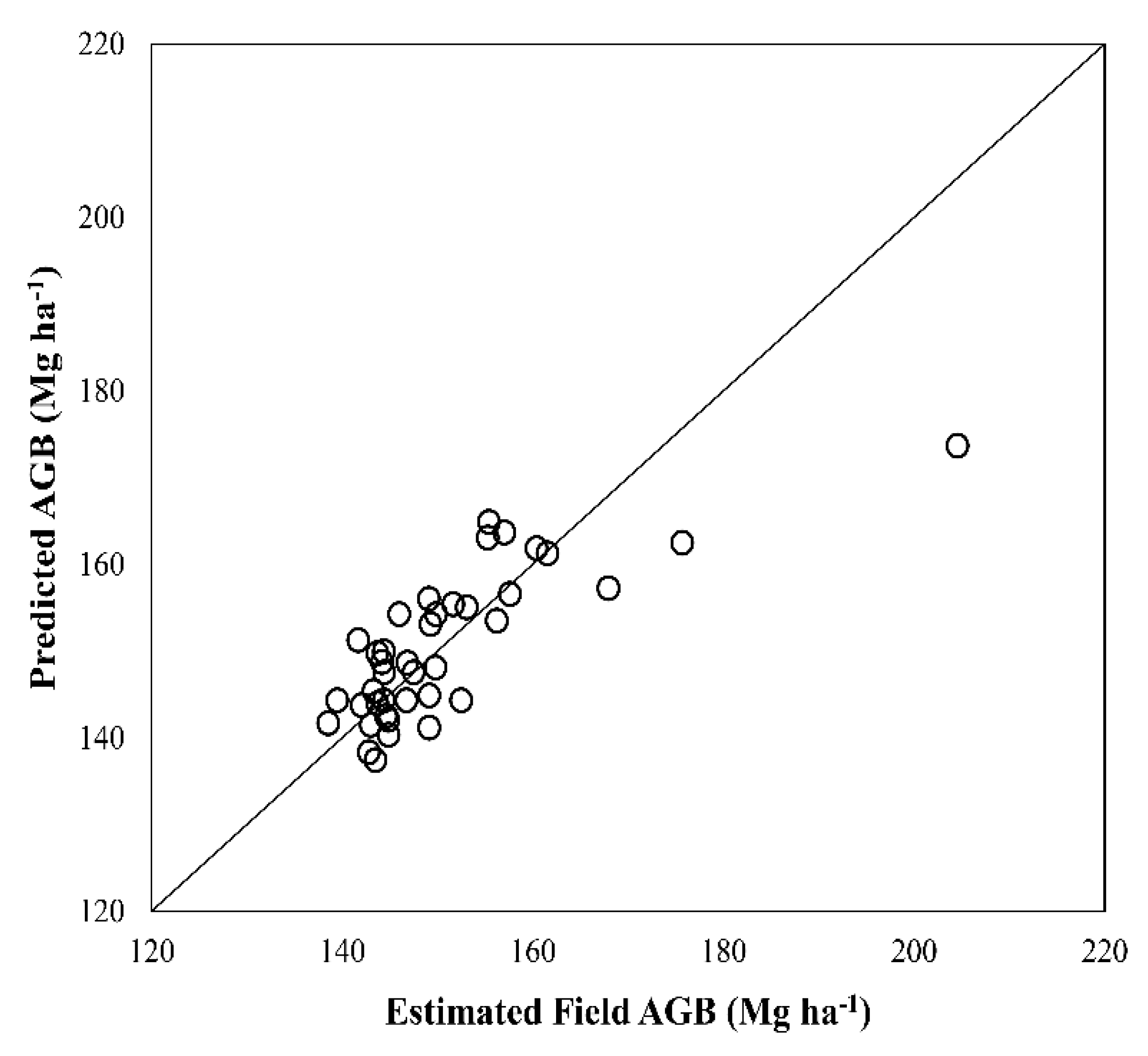
All forty plots were used in the regression analyses between the CHMs and the field AGB 2000. The results (Table 6) showed that the models with Ln AGB as the dependent variable and CHM as the independent variable had the highest R2 (0.60) for corrected and R2 (0.61) for uncorrected CHMs. The model with the uncorrected CHM as predictor had a RMSE of 8.24 Mg ha−1, or 5.47% of the average AGB (relative RMSE or RMSE%), and was slightly lower than the corrected CHM (RMSE = 8.39 Mg ha−1; RMSE% = 5.56%). Figure 6 shows the scatter-plot of AGB estimated from field data versus AGB predicted using the corrected CHM for the year 2000. The model was employed to produce a mangrove AGB map of Sabah for 2000. Sabah’s mangrove forest was estimated at 294,207.75 ha in 2000 with a total of 43,615,501.35 Mg of AGB. A total of 25,575.84 ha of mangrove forest had disappeared between 2000 and 2015 (1705.56 ha year−1). By multiplying the mangrove 2015 map with the AGB 2000 map, the mangrove AGB of 2015 was estimated at 39,652,659.26 Mg. This has translated into a significant decrease of more than 3.96 million Mg of mangrove AGB (or 1.98 million Mg of carbon with 0.5 conversion) in Sabah during the study period.

4. Discussion

4.1. Mangrove AGB Estimation Using Remotely Sensed Data

Mangrove AGB is conventionally examined based on field inventory despite the difficulties of accessing mangrove forests. We estimated AGB of mangrove forests of Sabah using field data and a published allometric equation. The observed AGB was about 196.88 Mg ha−1 while the estimated AGB was lower at 150.63 ha−1. These values fall within the range of average mangrove AGB in Malaysia. A study in Matang area, Peninsular Malaysia reported that the average AGB in Matang, which is dominated by Rhizophora apiculata species, was 185.30 Mg ha−1 [43]. In Sabah, the mangrove average AGB can be as low as 98.40 Mg ha−1 in the Kota Marudu district [44] and as high as 319 Mg ha−1 for the mangrove’s average AGB in the Sandakan district [45]. In the Lawas district of Sarawak, the neighboring state of Sabah, the mangrove average AGB is 116.79 Mg ha−1 [46]. The differences of AGB values in these different studies might be attributed to various factors, such as stem density and growth rate, as well as the disturbance history [46].
In recent years, mangrove AGB estimation over a spatially large area has focused on the correlation between mangrove canopy heights and remotely sensed height measurements, especially when using SRTM DSM or GLAS data. The approach generally involves the calibration of SRTM DSM values into canopy heights (e.g., [31,33]) or ICESat/GLAS generated heights (e.g., [27,34]), which are then used in AGB allometry. By calibrating SRTM DSM into tree height measurements using field data collected in 2005, mangrove AGB in Mozambique was estimated with a RMSE of 44 Mg ha−1 [31]. Aslan et al. [33] used the same approach to calibrate SRTM DSM to tree height measurements taken in 2013 but the RMSE, at 147.98 Mg ha−1, was considerably higher. In Colombia, mangrove AGB was estimated based on the linear relationship between ICEsat height estimates and SRTM elevation. The regression residual calculated using field data collected in 2005 was 17.3 Mg ha−1 [30]. In the case of Africa, applying the relative height of GLAS height measurements as canopy height to estimate mangrove AGB resulted in an RMSE of 65.4 Mg ha−1. It was calculated indirectly based on the RMSE of canopy height estimated with SRTM DSM [27]. This approach was later improved and used to estimate the global mangrove above-ground carbon stock with field data collected within 15 years after the SRTM data were obtained [34]. The time gap between field data and SRTM DSM data is one of the main error sources of AGB estimation using SRTM DSM [34]. The AGB growth during the gap could be substantial, even for mangroves that have a relatively slow growth rate.
There is a predictive relationship between annual AGB increment and AGB for tropical forest ecosystems [42]. A similar approach was employed to adjust the field AGB of different years to year 2000 and successfully estimate AGB of lowland mixed dipterocarp forests in Northern Borneo [47]. The iterative adjustment reduced the DBH and thus the number of trees in our field data. Nevertheless, only 250 trees or 7.6% of the total measured trees (3222 trees) were reduced after applying the adjustment. Based on our data, the mangrove AGB growth rate in Sabah was averagely 2.2 Mg ha−1 year−1. The AGB in 2000 might be underestimated as we did not consider any tree mortality that might have occurred before the field data collection. Without taking into consideration the time gap between the field measurements and SRTM CHM, the RMSE of mangrove AGB estimation in Sabah was 19.70 Mg ha−1 [48]. In this study, uncorrected SRTM DSM using a simulated DTM produced the best model for the AGB estimation in Sabah (RMSE 8.24 Mg ha−1). It is clearly shown that accounting for time gaps between field survey and digital elevation data leads to significant improvement in AGB prediction accuracy. The time-gap issue should therefore be addressed in future AGB studies. Nevertheless, the difference between corrected and uncorrected SRTM data is relatively small in comparison to the elevation errors reported for the global SRTM data, it is sufficient to assume a flat topography for mangrove AGB estimation using SRTM DSM as CHM [34].
With the recent advancement in remote sensing technology, digital elevation datasets have become increasingly available. These datasets have similar or higher spatial resolution, such as the ALOS PALSAR, and TanDEM-X data can be used as CHM for mangroves. Digital elevation data can also be generated using digital aerial photographs with the structure from motion technique. The use of these datasets for estimating AGB should be further examined in future.

4.2. Mangrove AGB Loss and Its Implications for REDD+ in Sabah, Malaysia

To map the mangrove forest changes between 2000 and 2015, we derived the mangrove forest areas based on supervised classification of Landsat image. Comparison of the classified mangrove forest area with existing statistics is not straightforward. Based on our classification, Sabah’s mangrove forest was estimated at 294,207.75 ha in 2000, compared to the estimate of 327,678 ha around the early 2000s given by Jakobsen et al. [17]. The overall accuracy (96.98%) and kappa coefficient (0.94) of our classification were high, while no accuracy was reported in Jakobsen et al. [17]. Based on the global mangrove dataset of the USGS, there were 284,952.27 ha of mangroves in Sabah in 2011. Our study found that the mangrove forest cover was 268,631.91 ha in 2015. Apart from mangrove deforestation, the differences in the mangrove area between other studies and our results could be due to the use of different satellite images and different cloud cover percentage, which needs to be removed. Gap filling can be conducted to fill in the removed areas, but is limited to available images. Moreover, the detection of mangrove areas that are partially submerged in the coastal waters may be restricted by the spatial resolution of the Landsat image [49].
The changes in mangrove forest cover reported in this study were based on the available Landsat images with low cloud and haze conditions. Most of the mangroves are found along the North to East coasts of Sabah (Figure 2). Overall, the mangrove area had decreased more than 25,000 ha within the 15-year study period. At a rate of 1705.56 ha per year (0.58% per year), losses are notably higher than the recent estimated global rate of mangrove loss, which ranges between 0.16% and 0.39% annually [13]. The deforestation rate might have been off-set by natural mangrove AGB colonization and small-scale mangrove replanting projects between 2011 and 2014 in the districts of Sandakan, Beluran, Beaufort and Kunak [50]. This study only considered the AGB changes due to deforestation, so the mangrove AGB changes were based on the estimated AGB and mangrove cover changes between 2000 and 2015. Overall, the mangrove AGB had decreased from 43,615,501.35 Mg in 2000 to 39,652,659.26 Mg in 2015. This means a significant decrease of more than 3.96 million Mg of mangrove AGB (or 1.98 million Mg Carbon with 0.5 conversion) at an annual rate of 264,189.47 Mg per year.
As the amendment of Sabah’s Forest Enactment 1968 to include REDD+ was passed in the state’s assembly and came into force in January 2019, the state government of Sabah clearly needs to adopt an effective strategy to conserve mangroves of Sabah. Recently, capacity building activities supported by a European Union fund have improved the Measurement, Reporting and Verification capacity of the state government. In addition, an above-ground carbon density map at 30 m resolution was developed for the forests except mangrove [51]. Mangrove is one of the five forest classes in the national forest reference emission level for REDD+ [15]. The AGB map of this study provides a baseline on the spatial distribution of mangrove AGB at sub-national level in 2000. Moreover, the mangrove AGB change map can be used to guide management decisions at policy or state level. For example, establishing new protection forest reserves or reclassifying existing reserves to protection forest reserves (Class I) at the threatened areas are an immediate and effective solution. Alternatively, the intensification of mangrove forest rehabilitation should also be carried out.

5. Conclusions

As mangrove areas in Sabah comprises of more than half of the total area of mangrove in Malaysia, baseline information on the mangrove area and its AGB is important to the mechanism of Reduce Emissions from Deforestation and Forest Degradation-Plus (REDD+) at sub-national, as well as national levels. In this study, we developed a predictive model to adjust field DBH measurements for determining the field AGB in 2000, when SRTM data was acquired. The historical mangrove AGB map in 2000 was produced by developing an AGB estimation model using the predicted field AGB and SRTM DSM corrected for ground elevation. Mangrove deforestation in Sabah between 2000 and 2015 was also quantified using multitemporal Landsat images. Although the mangrove deforestation rate was lower than the global rate, the total reduction of mangrove AGB or carbon stock was significant. The adjustment approach developed in this study can be applied to other regions covered by SRTM DSM to map the historical mangrove AGB in 2000.

Author Contributions

M.-H.P., K.U.K. and S.T. framed the research questions and designed the study. M.-H.P., N.A.B. and J.T. designed the field data collection, which was carried out by C.J.W. and D.J. Remotely sensed data processing and analysis were conducted by C.J.W. and D.J. C.J.W. prepared the first draft while M.-H.P., K.U.K. and S.T. reviewed and revised the manuscript. All authors have read and agreed to the published version of the manuscript.

Funding

This research was funded by Ministry of Higher Education (Project: NRGS0005), Ministry of Science, Technology and Innovation (Sciencefund: 04-01-10-SF0223) and Universiti Malaysia Sabah, Malaysia.

Acknowledgments

The authors would like to thank generous assistance and cooperation of various parties involved in this study. We would like to thank Sabah Forestry Department for research permission. Special thanks go to Nur Athirah Mohd Kamal, Nur Izzati Mohd Hanafiah, Jim Liew Jun Fei, Keiko Ioki and Wilson Wong for helping the field works.

Conflicts of Interest

The authors declare no conflict of interest.

References

  1. Baccini, A.; Goetz, S.J.; Walker, W.S.; Laporte, N.T.; Sun, M.; Sulla-Menashe, D.; Hackler, J.; Beck, P.S.A.; Dubayah, R.; Friedl, M.A.; et al. Estimated carbon dioxide emissions from tropical deforestation improved by carbon-density maps. Nat. Clim. Chang. 2012, 2, 182–185. [Google Scholar] [CrossRef]
  2. UN-REDD. The UN-REDD Programme Strategy 2011–2015; UN-REDD: Geneva, Switzerland, 2011. [Google Scholar]
  3. Gibbs, H.K.; Brown, S.; Niles, J.O.; Foley, J.A. Monitoring and estimating tropical forest carbon stocks: Making REDD a reality. Environ. Res. Lett. 2007, 2, 1–3. [Google Scholar] [CrossRef]
  4. UNFCCC. Executive Board Annual Report 2014: Clean Development Mechanism; United Nations Framework Convention on Climate Change: Luxembourg, 2014. [Google Scholar]
  5. Dahdouh-Guebas, F. World Atlas of Mangroves: Mark Spalding, Mami Kainuma and Lorna Collins (eds). Hum. Ecol. 2011, 39, 107–109. [Google Scholar] [CrossRef]
  6. Castillo, J.A.A.; Apan, A.A.; Maraseni, T.N.; Salmo, S.G. Soil C quantities of mangrove forests, their competing land uses, and their spatial distribution in the coast of Honda Bay, Philippines. Geoderma 2017, 293, 82–90. [Google Scholar] [CrossRef]
  7. Donato, D.C.; Kauffman, J.B.; Murdiyarso, D.; Kurnianto, S.; Stidham, M.; Kanninen, M. Mangroves among the most carbon-rich forests in the tropics. Nat. Geosci. 2011, 4, 293–297. [Google Scholar] [CrossRef]
  8. Pham, L.T.H.; Brabyn, L. Monitoring mangrove biomass change in Vietnam using SPOT images and an object-based approach combined with machine learning algorithms. ISPRS J. Photogramm. Remote Sens. 2017, 128, 86–97. [Google Scholar] [CrossRef]
  9. Kauffman, J.B.; Heider, C.; Cole, T.G.; Dwire, K.A.; Donato, D.C. Ecosystem carbon stocks of Micronesian mangrove forests. Wetlands 2011, 31, 343–352. [Google Scholar] [CrossRef]
  10. Stringer, C.E.; Trettin, C.C.; Zarnoch, S.J.; Tang, W. Carbon stocks of mangroves within the Zambezi River Delta, Mozambique. For. Ecol. Manag. 2015, 354, 139–148. [Google Scholar] [CrossRef]
  11. Kanniah, K.D.; Sheikhi, A.; Cracknell, A.P.; Goh, H.C.; Tan, K.P.; Ho, C.S.; Rasli, F.N. Satellite images for monitoring mangrove cover changes in a fast growing economic region in Southern Peninsular Malaysia. Remote Sens. 2015, 7, 14360–14385. [Google Scholar] [CrossRef] [Green Version]
  12. Barros, D.F.; Albernaz, A.L.M. Possible impacts of climate change on wetlands and its biota in the Brazilian Amazon. Braz. J. Biol. 2014, 74, 810–820. [Google Scholar] [CrossRef]
  13. Hamilton, S.E.; Casey, D. Creation of a high spatio-temporal resolution global database of continuous mangrove forest cover for the 21st century (CGMFC-21). Glob. Ecol. Biogeogr. 2016, 25, 729–738. [Google Scholar] [CrossRef]
  14. Hamilton, S.E.; Friess, D.A. Global carbon stocks and potential emissions due to mangrove deforestation from 2000 to 2012. Nat. Clim. Chang. 2018, 8, 240–244. [Google Scholar] [CrossRef] [Green Version]
  15. Ministry of Natural Resources and Environment Malaysia (NRE). Second National Communication to the UNFCCC; NRE: Putrajaya, Malaysia, 2011. [Google Scholar]
  16. Food and Agriculture Organization of the United Nations (FAO). Brief on National Forest Inventory (NFI): Malaysia; FAO: Rome, Italy, 2007. [Google Scholar]
  17. Jakobsen, F.; Hartstein, N.; Frachisse, J.; Golingi, T. Sabah shoreline management plan (Borneo, Malaysia): Ecosystems and pollution. Ocean. Coast. Manag. 2007, 50, 84–102. [Google Scholar] [CrossRef]
  18. Saenger, P.; Snedaker, S.C. Pantropical trends in mangrove above-ground biomass and annual litterfall. Oecologia 1993, 96, 293–299. [Google Scholar] [CrossRef] [PubMed] [Green Version]
  19. Kamlun, K.U.; Arndt, R.B.; Phua, M.H. Monitoring deforestation in Malaysia between 1985 and 2013: Insight from South-Western Sabah and its protected peat swamp area. Land Use Policy 2016, 57, 418–430. [Google Scholar] [CrossRef]
  20. Phua, M.H.; Tsuyuki, S.; Lee, J.S.; Ghani, M. Simultaneous detection of burned areas of multiple fires in the tropics using multisensor remote sensing data. Int. J. Remote Sens. 2012, 33, 4312–4333. [Google Scholar] [CrossRef]
  21. Rahman, M.M.; Khan, M.N.I.; Hoque, A.F.; Ahmed, I. Carbon stocks in the Sundurbans mangrove forest: Spatial variations in vegetation types and salinity zones. Wetl. Ecol. Manag. 2015, 23, 269–283. [Google Scholar] [CrossRef]
  22. Tokola, T. Remote sensing concepts and their applicability in REDD+ monitoring. Curr. For. Rep. 2015, 1, 252–260. [Google Scholar] [CrossRef] [Green Version]
  23. Saatchi, S.S. Synergism of optical and radar data for forest structure and biomass. Ambiencia Guarapuava 2010, 6, 151–166. [Google Scholar]
  24. Englhart, S.; Keuck, V.; Siegert, F. Aboveground biomass retrieval in tropical forests—The potential of combined X- and L-band SAR data use. Remote Sens. Environ. 2011, 115, 1260–1271. [Google Scholar] [CrossRef]
  25. Ioki, K.; Tsuyuki, S.; Hirata, Y.; Phua, M.H.; Wong, W.V.C.; Ling, Z.Y.; Saito, H.; Takao, G. Estimating above-ground biomass of tropical rainforest of different degradation levels in Northern Borneo using airborne LiDAR. For. Ecol. Manag. 2014, 328, 335–341. [Google Scholar] [CrossRef]
  26. Phua, M.H.; Hue, S.W.; Ioki, K.; Hashim, M.; Bidin, K.; Musta, B.; Suleiman, M.; Yap, S.W.; Maycock, C.R. Estimating logged-over lowland rainforest aboveground biomass in Sabah, Malaysia using airborne LiDAR data. Terr. Atmos. Ocean. Sci. 2016, 27, 481–489. [Google Scholar] [CrossRef] [Green Version]
  27. Fatoyinbo, T.E.; Simard, M. Height and biomass of mangroves in Africa from ICESat/GLAS and SRTM. Int. J. Remote Sens. 2013, 34, 668–681. [Google Scholar] [CrossRef]
  28. Lagomasino, D.; Fatoyinbo, T.; Lee, S.K.; Feliciano, E.; Trettin, C.; Simard, M. A comparison of mangrove canopy height using multiple independent measurements from land, air, and space. Remote Sens. 2016, 8, 327. [Google Scholar] [CrossRef] [PubMed] [Green Version]
  29. Simard, M.; Zhang, K.; Rivera-Monroy, V.H.; Ross, M.S.; Ruis, P.L.; Castaneda-Moya, E.; Twilley, R.R.; Rodriguez, E. Mapping height and biomass of mangrove forests in Everglades National Park with SRTM elevation data. Photogramm. Eng. Remote Sens. 2006, 72, 299–311. [Google Scholar] [CrossRef]
  30. Simard, M.; Rivera-Monroy, V.H.; Mancera-Pineda, J.E.; Castaneda-Moya, E.; Twilley, R.R. A systematic method for 3D mapping of mangrove forests based on Shuttle Radar Topography Mission elevation data, ICEsat/GLAS waveforms and field data: Application to Ciénaga Grande de Santa Marta, Colombia. Remote Sens. Environ. 2008, 112, 2131–2144. [Google Scholar] [CrossRef]
  31. Fatoyinbo, T.E.; Simard, M.; Washington-Allen, R.A.; Shugart, H.H. Landscape-scale extent, height, biomass, and carbon estimation of Mozambique’s mangrove forests with Landsat ETM + and Shuttle Radar Topography Mission elevation data. J. Geophys. Res. Biogeosci. 2008, 113, 1–13. [Google Scholar] [CrossRef]
  32. Fayad, I.; Baghdadi, N.; Guitet, S.; Bailly, J.S.; Herault, B.; Gond, V.; El Hajj, M.; Minh, D.H.T. Aboveground biomass mapping in French Guiana by combining remote sensing, forest inventories and environmental data. Int. J. Appl. Earth. Obs. Geoinf. 2016, 52, 502–514. [Google Scholar] [CrossRef] [Green Version]
  33. Aslan, A.; Rahman, A.F.; Warren, M.W.; Robeson, S.M. Mapping spatial distribution and biomass of coastal wetland vegetation in Indonesian Papua by combining active and passive remotely sensed data. Remote Sens. Environ. 2016, 183, 65–81. [Google Scholar] [CrossRef]
  34. Simard, M.; Fatoyinbo, L.; Smetanka, C.; Rivera-Monroy, V.H.; Castaneda-Moya, E.; Thomas, N.; Van der Stocken, T. Mangrove canopy height globally related to precipitation, temperature and cyclone frequency. Nat. Geosci. 2019, 12, 40–45. [Google Scholar] [CrossRef]
  35. Sabah Forestry Department. Sabah Forestry Department Annual Report 2015; SFD: Sandakan, Malaysia, 2016. [Google Scholar]
  36. Chave, J.; Rejou-Mechain, M.; Burquez, A.; Chidumayo, E.; Colgan, M.S.; Delitti, W.B.C.; Duque, A.; Eid, T.; Fearnside, P.M.; Goodman, R.C.; et al. Improved allometric models to estimate the aboveground biomass of tropical trees. Glob. Chang. Biol. 2014, 20, 3177–3190. [Google Scholar] [CrossRef] [PubMed]
  37. Clark, D.A.; Brown, S.; Kicklighter, D.W.; Chambers, J.Q.; Thomlinson, J.R.; Ni, J.; Holland, E. Net primary production in tropical forests: An evaluation and synthesis of existing field data. Ecol. Appl. 2011, 11, 371–384. [Google Scholar] [CrossRef]
  38. U.S. Geological Survey. Available online: http://glovis.usgs.gov (accessed on 5 February 2018).
  39. U.S. Geological Survey. Available online: http://earthexplorer.usgs.gov (accessed on 7 November 2017).
  40. DHI Water and Environment. Sabah Shoreline Management Plan; DHI Water and Environment: Kota Kinabalu, Malaysia, 2005. [Google Scholar]
  41. Basuki, T.M.; van Laake, P.E.; Skidmore, A.K.; Hussin, Y.A. Allometric equations for estimating the above-ground biomass in tropical lowland Dipterocarp forests. For. Ecol. Manag. 2019, 257, 1684–1694. [Google Scholar] [CrossRef]
  42. Yamakura, T.; Hagihara, A.; Sukardjo, S.; Ogawa, H. Aboveground biomass of tropical rain forest stands in Indonesian Borneo. Vegetatio 1986, 68, 71–82. [Google Scholar] [CrossRef]
  43. Gong, W.K.; Ong, J.E. Plant biomass and nutrient flux in a managed mangrove forest in Malaysia. Estuar. Coast. Shelf Sci. 1990, 31, 519–530. [Google Scholar] [CrossRef]
  44. Faridah-Hanum, I.; Kudus, K.A.; Saari, N.S. Plant diversity and biomass of Marudu Bay mangroves in Malaysia. Pak. J. Bot. 2012, 44, 151–156. [Google Scholar]
  45. Tangah, J.; Nilus, R.; Sugau, J.B.; Titin, J.; Paul, V.; Yahya, F.; Suis, M.A.F.; Chung, A.Y.C. The establishment of long term ecological research plots in the Sepilok mangroves. Sepilok Bull. 2018, 27, 1–22. [Google Scholar]
  46. Chandra, I.A.; Seca, G.; Hena, M.K.A. Aboveground biomass production of Rhizophora apiculata blume in Sarawak mangrove forest. Am. J. Agric. Biol. Sci. 2011, 6, 469–474. [Google Scholar]
  47. Langner, A.; Samejima, H.; Ong, R.C.; Titin, J.; Kitayama, K. Integration of carbon conservation into sustainable forest management using high resolution satellite imagery: A case study in Sabah, Malaysian Borneo. Int. J. Appl. Earth. Obs. Geoinf. 2012, 18, 305–312. [Google Scholar] [CrossRef]
  48. Wong, C.J.; Besar, N.A.; James, D.; Phua, M.H. Estimating mangrove above-ground biomass in Sabah using SRTM DSM, Landsat and field data. J. Korean For. Soc. 2020, in press. [Google Scholar]
  49. Kirui, K.B.; Kairo, J.G.; Bosire, J.; Viergever, K.M.; Rudra, S.; Huxham, M.; Briers, R.A. Mapping of mangrove forest land cover change along the Kenya coastline using Landsat imagery. Ocean. Coast. Manag. 2013, 83, 19–24. [Google Scholar] [CrossRef]
  50. Tangah, J.; Bajau, F.E.; Jilimin, W.; Baba, S.; Chan, H.T.; Kesuka, M. Rehabilitation of Mangrove in Sabah-The SFD-ISME Collaboration (2011–2014); Sabah Forestry Department: Kota Kinabalu, Malaysia, 2015. [Google Scholar]
  51. Asner, G.P.; Brodrick, P.G.; Philipson, C.; Vaughn, N.R.; Martin, R.E.; Knapp, D.E.; Heckler, J.; Evans, L.J.; Jucker, T.; Goossens, B.; et al. Mapped aboveground carbon stocks to advance forest conservation and recovery in Malaysian Borneo. Biol. Conserv. 2018, 217, 289–310. [Google Scholar] [CrossRef]
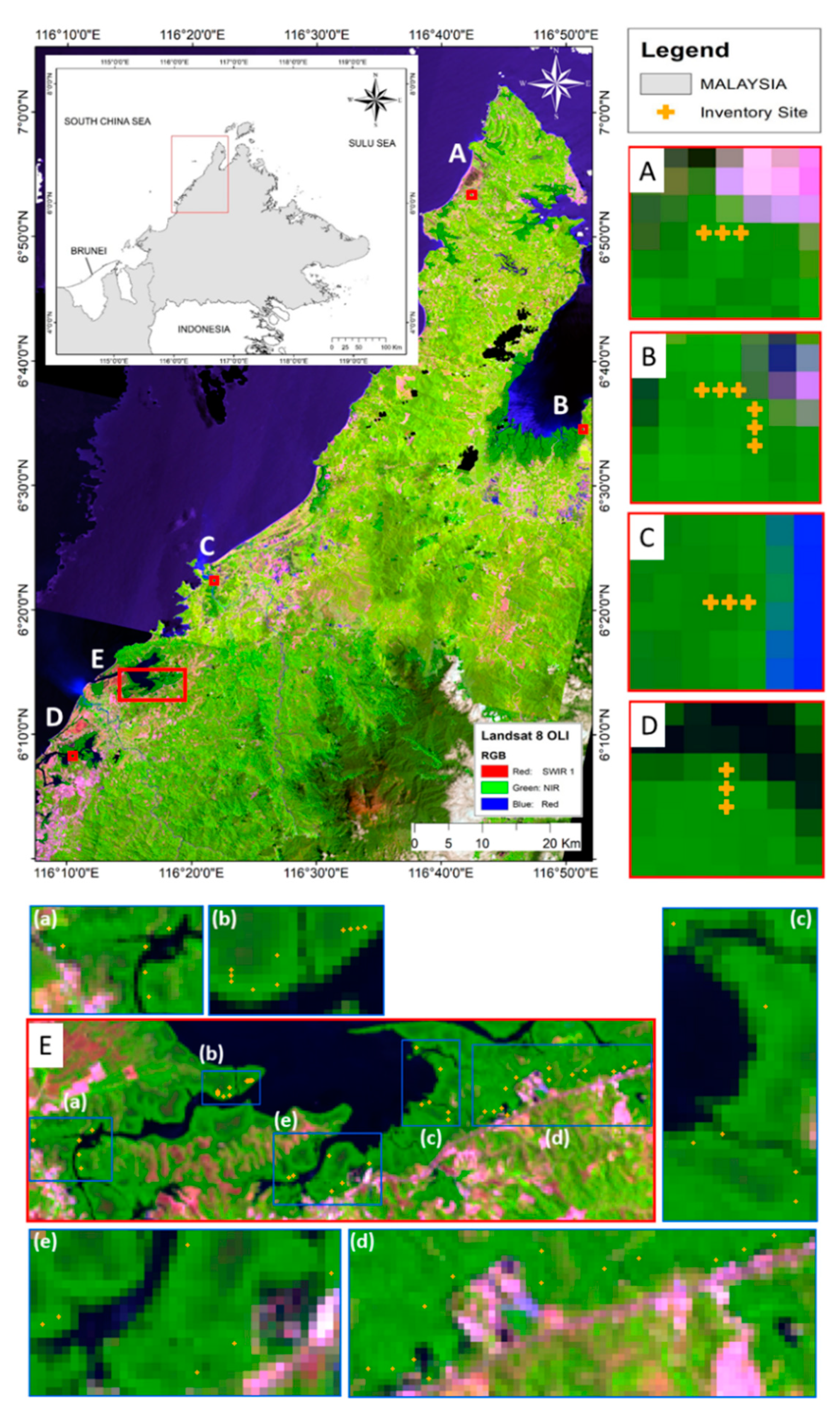
Figure 1. Location of the study area (top part). Field plot locations are plotted as cross (+) in yellow on a Landsat7 image of 2015.
Forests 11 01018 g001
Figure 2. Relationship between DBH and annual DBH increment at tree level in Sabah (n = 347). Compared to the plot-level approach in [37], considerable variations in DBH increment can be observed at tree level, but the annual rate is clearly dependent on the tree DBH.
Forests 11 01018 g002
Figure 3. DBH and height relationship of mangrove trees in Sabah (n = 2760).
Forests 11 01018 g003
Figure 4. Relationship between distance from coastline and elevation above mean sea level (n = 362).
Forests 11 01018 g004
Figure 5. Changes in mangrove forest cover in Sabah between 2000 and 2015.
Forests 11 01018 g005
Figure 6. Estimated field AGB vs. predicted AGB. Only one plot was considerably underestimated.
Forests 11 01018 g006
Table 1. Regression Statistics of Diameter at Breast Height (DBH) Increment Estimation Model.
ModelDBH Increment = 0.787ln(DBH) − 1.404
No of Samples (n)347
R0.67
R20.44
ConstantVariable Coefficients
B−1.4040.787
SE0.2280.090
t−6.1598.723
Sig.0.000 *0.000 *
Notes: B, regression coefficient; SE, standard error; t, Student’s t statistic; Sig., significance value. * Significant at the 0.001 level.
Table 2. Regression Statistics of the Height Estimation Model.
ModelHeight = 3.100(DBH)0.623
No of Samples (n)2760
R0.76
R20.58
ConstantVariable Coefficients
B3.1000.623
SE0.0750.010
t41.17661.991
Sig.0.000 *0.000 *
Notes: B, regression coefficient; SE, standard error; t, Student’s t statistic; Sig., significance value. * Significant at the 0.001 level.
Table 3. Regression Statistics of the Digital Terrain Model (DTM) Estimation Model.
ModelDTMmg = 0.019 (D) + 0.343
No of Samples (n)362
R0.73
R20.54
ConstantVariable Coefficients
B0.3430.019
SE0.0890.001
t3.87020.482
Sig.0.000 *0.000 *
Notes: B, regression coefficient; SE, standard error; t, Student’s t statistic; Sig., significance value. * Significant at the 0.001 level.
Table 4. Classification Accuracy for Mangrove 2000 and 2015.
(a) 2000GroundtruthsLine TotalUser’s Accuracy (%)
MangroveNon Mangrove
ClassificationMangrove136113799.27
Non Mangrove918519495.36
Column Total 145186331
Producer’s Accuracy (%) 93.7999.46
Overall Accuracy = 96.98%; Overall Kappa = 0.94
(b) 2015GroundtruthsLine TotalUser’s Accuracy (%)
MangroveNon Mangrove
ClassificationMangrove114411896.61
Non Mangrove1619521192.42
Column Total 130199329
Producer’s Accuracy (%) 87.6997.99
Overall Accuracy = 93.92%; Overall Kappa = 0.87
Table 5. Summary of the Observed and Estimated Field Variables Mangrove Forest in the Study Area.
DBH (cm)Height (m)AGB (Mg ha−1)
AverageObserved11.8914.30196.88
Estimated7.0810.45150.63
MinimumObserved5.02.65135.61
Estimated5.959.41138.52
MaximumObserved4930.95291.31
Estimated25.9823.58204.54
Standard DeviationObserved5.444.4332.58
Estimated1.551.2811.66
Table 6. Summary of Above-Ground Biomass (AGB) Estimation Models Using Corrected and Uncorrected Shuttle Radar Topography Mission (SRTM) Canopy Height Models (CHMs).
VariablesRR2Model EquationRMSE Mg ha−1% RMSE
CorrectedAGB – CHM0.760.57AGB = 2.51(CHM) + 128.288.595.70
AGB – Ln CHM0.680.46AGB = 20.07(Ln CHM) + 108.249.366.21
Ln AGB – CHM0.770.60Ln AGB = 0.02(CHM) + 4.878.385.56
UncorrectedAGB – CHM0.770.59AGB = 2.38(CHM) + 123.928.475.62
AGB – Ln CHM0.690.47AGB = 23.78(Ln CHM) + 94.479.266.15
Ln AGB – CHM0.780.61Ln AGB = 0.01(CHM) + 4.858.245.47