Article

Direct Versus Indirect Tree Ring Reconstruction of Annual Discharge of Chemora River, Algeria

1
Laboratory of Tree Ring Research, University of Arizona, Tucson, AZ 85721, USA
2
Institute of Veterinary and Agronomy Sciences, The University Batna 1 Hadj-Lakhdar, Batna 05000, Algeria
3
Faculty of Biological Sciences and Agronomy, The University Mouloud Mammeri, Tizi Ouzou 15000, Algeria
*
Author to whom correspondence should be addressed.
Forests 2020, 11(9), 986; https://doi.org/10.3390/f11090986
Submission received: 14 August 2020 / Revised: 7 September 2020 / Accepted: 7 September 2020 / Published: 14 September 2020
(This article belongs to the Special Issue Dendroecological Wood Anatomy and Xylogenesis)

Abstract

:
Annual river discharge is a critical variable for water resources planning and management. Tree rings are widely used to reconstruct annual discharge, but errors can be large when tree growth fails to respond commensurately to hydrologically important seasonal components of climate. This paper contrasts direct and indirect reconstruction as statistical approaches to discharge reconstruction for the Chemora River, in semi-arid northeastern Algeria, and explores indirect reconstruction as a diagnostic tool in reconstruction error analysis. We define direct reconstruction as predictions from regression of annual discharge on tree ring data, and indirect reconstruction as predictions from a four-stage process: (1) regression of precipitation on tree rings, (2) application of the regression model to get reconstructed precipitation for grid cells over the basin, (3) routing of reconstructed precipitation through a climatological water balance (WB) model, and (4) summing model runoff over cells to get the reconstructed discharge at a gage location. For comparative purposes, the potential predictors in both modeling approaches are the same principal components of tree ring width chronologies from a network of drought-sensitive sites of Pinus halepensis and Cedrus atlantica in northern Algeria. Results suggest that both modeling approaches can yield statistically significant reconstructions for the Chemora River. Greater accuracy and simplicity of the direct method are countered by conceptual physical advantages of the indirect method. The WB modeling inherent to the indirect method is useful as a diagnostic tool in error analysis of discharge reconstruction, points out the low and declining importance of snowmelt to the river discharge, and gives clues to the cause of severe underestimation of discharge in the outlier high-discharge year 1996. Results show that indirect reconstruction would benefit most in this basin from tree ring resolution of seasonal precipitation.

1. Introduction

Tree ring reconstructions of river discharge have long been used to place recent and projected hydroclimatic variability in a multi-century context [1,2]. Hydrologic models have proved useful for improved understanding of the variability. For example, tree ring reconstructions of river discharge routed through a lake water-balance (WB) model helped corroborate multi-century droughts in the Sierra Nevada of California inferred from radiocarbon-dated stumps exposed in rivers and lakes [3]. Hydrologic models have recently been incorporated into the statistical models for discharge reconstruction. The central idea is to statistically reconstruct climatic variables, such as precipitation (P) and temperature (T), that directly impact tree growth, and then use the reconstructed variables as inputs to a physically based hydrologic model whose output includes runoff or river discharge [4,5,6,7]. We call such reconstruction of discharge through the intermediary of a hydrologic model “indirect” reconstruction, and the alternative more straightforward approach of regressing the target observed discharge time series on tree ring time series [8,9,10,11] “direct” reconstruction.
An advantage of indirect over direct reconstruction is the possibility of reconstructing discharge for rivers with very short or no existing gaged discharge records. Another is the investigation of alternative past P and T scenarios to explain low-growth or high-growth episodes in the tree ring record. A disadvantage of indirect reconstruction is the data requirement. The hydrologic model for indirect reconstruction requires seasonal [5] or monthly [7] time series inputs of observed and reconstructed climate variables. Representative climatic data may not be available for some basins. Tree ring data capable of resolving P and T signals at seasonal resolution may also be lacking. Some basins may also lack a suitable gaged discharge record for calibrating the water-balance model, although application of uncalibrated WB models has also been shown to yield insights to hydroclimatic variability [12].
Comparative studies of direct and indirect reconstruction are lacking. In this paper, we address the strengths and weaknesses of direct versus indirect reconstruction of annual discharge of the Chemora River, northeastern Algeria. The basin was selected specifically because it is relatively small, semi-arid, and yet well sampled with a network of P stations covering more than 40 years. Moreover, field collections over the past few decades have yielded a network of drought-sensitive tree ring chronologies—several close to the basin—in northeastern Algeria [13]. The direct and indirect reconstructions compared here draw their predictors from the same network of tree ring sites: total-width chronologies of Pinus halepensis and Cedrus atlantica. Results show that consistent reconstructions for the Chemora River can be derived both directly and indirectly. The direct reconstruction is more accurate and less biased than the indirect reconstruction, but the indirect approach offers valuable insight into past hydrologic conditions.

2. Study Basin

The study basin is the semi-arid Chemora River Basin in northeastern Algeria (Figure 1a). The basin has an area of 759 k m 2 , and includes rugged terrain ranging in elevation from 2311 m on Djebel El Mahmel to 890 m on the salt flats at the river outlet [14]. The Chemora River is formed by the confluence of the Reboa and Soultez Rivers, which drain from the south and west, respectively (Figure 1b). The climate is Mediterranean, with cold wet winters and dry summers. Mean annual P in most of the basin is 300 m m to 450 m m , but exceeds 600 m m at the highest elevations [15]. The estimated equivalent average annual depth of P over the basin is 370 m m [14].
Cultivated cropland, mainly for grain farming, occupies most of the watershed [14]. The native forest cover has been severely degraded; dense forest, mainly Pinus halepensis and Quercus ilex, is now localized to the elevation zone 1200 m to 1800 m in the southwestern part of the basin [14]. The piedmonts, as well as those parts of the mountains where forests have disappeared, are occupied by rangeland and barren ground [14].
Low average P and a highly variable climate make water a scarce resource in the basin. In response, the National Agency for Dams and Transfer (NADT) of Algeria built the Koudiet Lamdaouar Dam in the early 2000s. The reservoir capacity of 74 × 106 m 3 [16] provides storage equivalent to more than three years of annual average discharge of the Chemora River. Storage behind this dam severely distorts gaged flows downstream starting with water year 2003.

3. Materials and Methods

3.1. Hydrologic, Climatic, and Tree Ring Data

Monthly mean gaged discharge (Q) of the Chemora River at Tkabaout for water years 1971–2005 was obtained from the National Agency of Water Resources, Algeria. Discharge data used in this study were restricted to 1971–2002 in view of the aforementioned influence of Koudiet Lamdaouar Dam. Gaged Q even before 2003 likely departs considerably from natural flows because of unrecorded diversion of river water for irrigation and other purposes in the heavily agricultural basin. Mean annual Q at Tkabaout is 0.69 m 3 s 1 , with the monthly maximum and minimum typically occurring in early spring and late summer, respectively (Figure 2).
Climatological data for the study consist of monthly station total P and average T. Monthly P data for 15 stations in or near the Chemora Basin (Figure 1a) were obtained from the National Agency of Water Resources, Algeria. These records cover water years 1969–2012 with no more than five years of data missing at any station for any month of the year. Station elevations range from 1000 m to 1650 m with a median of 1180 m . The similar shapes of the monthly distributions of Q at Tkabaout and P at the highest elevation station suggest that a delay of runoff ( R O ) by snowpack storage of P is not a major factor in the water balance of this basin (Figure 2). Adjusted Global Historical Climate Network (GHCN) monthly T for six stations, including one at Batna (from here on, Batna1) with much missing data, was downloaded from KNMI Explorer [17]. An additional Batna monthly T series (from here on, Batna2), serially complete for 1950–2015, was obtained from the National Office of Meteorology, Algeria, for the purpose of filling in missing data at Batna1.
A digital elevation model (DEM) was needed for adjustment of monthly station P and T to elevations of the grid cells of the WB model. From results of a study in Australia [18], we decided that a 5–10 km resolution is sufficient for assessing elevation dependence of monthly P in the Chemora Basin. Accordingly, we downloaded the ETOPO2v2 dataset from the website of the NOAA National Centers for Environmental Information [19] for this purpose (Figure 1b).
Tree ring data used consist of 23 standard site chronologies [20] whose locations are mapped in Figure 1a. The eight Pinus halepensis and fifteen Cedrus atlantica chronologies in this network are listed along with chronology statistics in Table A1. Chronologies were standardized using program ARSTAN [21] by conventional methods designed to emphasize the common growth signal and retain lower frequency climate information [22,23]. Development of the chronologies and assessment of their signal for P and T have been described elsewhere [13,24,25], and key details of standardization are repeated in Appendix A.1. The common period of coverage by the 23 chronologies is 1853–2005 CE.
To reduce redundancy in the tree ring network and emphasize major spatial modes of growth in preparation for reconstruction of discharge, a principal components analysis (PCA) was run on the 23 chronologies for the period 1853–2005. The PCA was run on the correlation matrix of the chronologies, and the important principal components (PCs) were identified with guidance from the “eigenvalue of 1” criterion and a scree plot of eigenvalues [26]. The important PCs comprised the pool of potential predictors for reconstruction models described in Section 3.3.

3.2. Water-Balance Model

The water-balance (WB) model used in this study is the Thornthwaite [27,28] monthly WB model, as adapted for numerous hydrologic studies on the scale of basins to continents [12,29,30]. This model has previously been applied in dendrochronology to enhance the interpretation of past droughts and wet periods [6], and as a tool for indirect reconstruction of runoff and river discharge [5,7]. The Thornthwaite model has a history of application in dendroclimatology as the framework for computation of the Palmer Drought Severity Index [31,32,33]. In this model, the monthly water balance for a soil column is
R O = P A E T Δ S
where R O is total runoff, P is precipitation, A E T is actual evapotranspiration, and Δ S is the change in water storage in the soil and overlying snowpack. The R O term is assumed to include surface and subsurface runoff. Over a sufficiently long time step the summation of R O over an area (e.g., watershed) should approximate river discharge. The approximation could be degraded by surface storage upstream of the gage, delayed groundwater contribution to river flow, capture of runoff by closed basins, or storage of runoff in aquifers not draining to the river above the gage.
Time series inputs required by the WB model are monthly P and monthly mean T (Figure A2). A fraction of the monthly P is assigned to direct runoff, and the remainder enters the soil–moisture balance, where it is subject to evapotranspiration. T influences several key water-balance components: potential evapotranspiration ( P E T ), which is estimated by the Hamon equation [34]; the fraction of P assigned as snowfall; and melting of the snowpack. A E T depends on both P E T and the soil moisture. Excess soil moisture (above a specified capacity) becomes surplus runoff. The total of direct and surplus runoff eventually contributes to river discharge.
Other inputs to the WB model include the latitude, which is used in the computation of day length and P E T , and the soil water capacity, which is related to the depth of the soil column. The user specifies settings for a small number of parameters controlling snow accumulation, snowmelt, and runoff. The WB-model equations are described in detail elsewhere [35] and are not repeated here. Parameter settings specific to our study are given in Appendix A.2.
The geographical domain for the WB modeling is the 154-cell rectangular 2 × 2 grid including the Chemora River Basin (Figure 1b). The necessary grid-cell input of monthly P and T was derived from station climate data. Monthly P at the 154 cells was interpolated by inverse distance weighting [36] of station P for 15 stations in or near the basin (Figure 1a). Simple linear regression models [37] of long-term monthly means and coefficients of variation of station P against station elevation were used to convert the interpolated standardized anomalies to original P units.
For monthly T, which is generally more spatially correlated than P, we assumed that the interannual variability of standardized T anomalies is sufficiently represented by the record from Batna1. The monthly grid-cell means of T were specified as equal the monthly means at Batna1 scaled using a seasonally varying lapse rate [38] to account for the elevation difference between Batna and the grid-cell centers. It was also necessary to consider the elevation dependence of the monthly standard deviation of T. We did this using linear regression [37] equations of station monthly coefficient of variation of T on station elevation for the six GHCN stations (Figure 1a). Steps for converting station monthly P and T to the grid-cell inputs for WB modeling are described in more detail in Appendix A.3.
The WB model was run on monthly input P and T, 1969–2012. Runoff summed over the 91 cells in the basin was defined as model discharge for comparison with gaged discharge at the Tkabaout gage. Because of aforementioned shortness of records and possible departure of the Tkabaout gaged record from natural flows, we did not attempt to optimize model parameters by calibrating the WB model to force model Q to approach gaged Q. We did, however, use the Tkabaout gaged Q to broadly judge the performance of the model using default parameter settings. To evaluate the importance of interannual T variation to discharge, the WB model was repeated on the 1969–2012 observed P, but with T held constant from year to year at the 1969–2012 long-term monthly means. The WB model was also run on two alternative paleoclimatic scenarios for indirect reconstruction as discussed in the next section.

3.3. Reconstruction

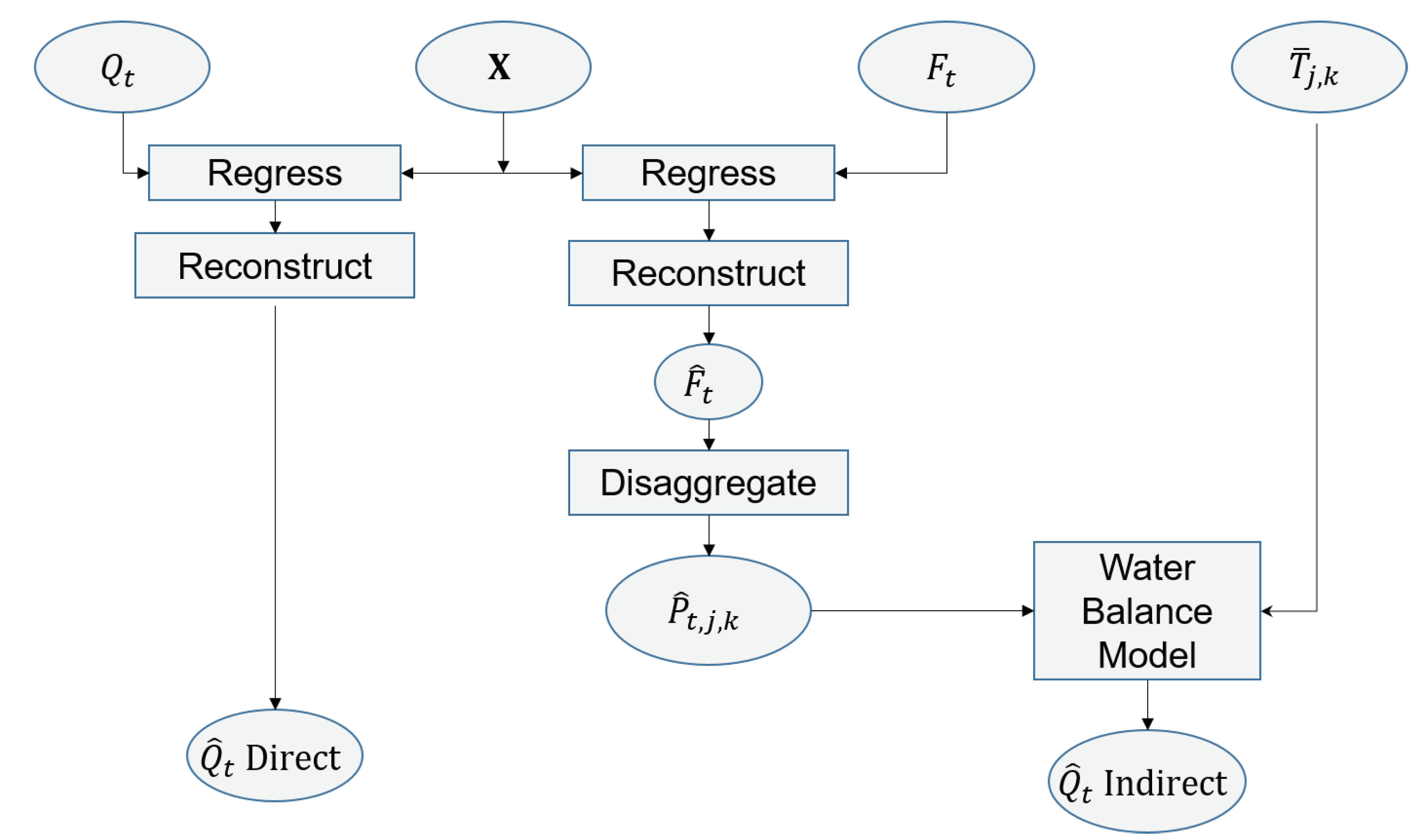
Direct and indirect reconstruction are contrasted in the schematic in Figure 3. The first approach is “direct” in that a regression equation directly links the predictand Q with tree ring predictors. The second approach is “indirect” in that the regression predictand is not Q itself, but is instead some climatic variable, assumed to be more directly sensed by tree growth, that can be input into a hydrologic model to generate reconstructed Q.
The statistical model for both reconstruction approaches in this study is the same:
y t = b 0 + i = 1 K b i x t , i + e t
where y t is the regression predictand in year t, x t , i are predictors, e t is the error term, and b 0 , b 1 , , b K are the regression constant and coefficients, which are to be estimated by regression such that the sum of squares of residuals (estimated error term) is minimized. The predictors for the model are selected by stepwise regression [39] using a p-to-enter of 0.05 and p-to-remove of 0.10. To facilitate comparison of methods, the calibration period and pool of potential predictors is kept the same for RecD and RecI. The key difference in the approaches is the predictand, y. For RecD, y is annual (water-year) Q; for RecI, y is PC1 of annual P at the 15 basin stations.
Once the regression parameters are estimated, the full reconstruction is generated by substituting available time series of tree ring predictors into the fitted equation y ^ t = b ^ 0 + i = 1 K b ^ i x t , i . The calibration residuals are defined by e ^ t = y y ^ , the difference of observed and predicted y for the period used to fit the model. An analysis of residuals was done to check that e t ^ satisfied regression assumptions on normality, lack of autocorrelation, and constancy of variance [39]. Models were then cross-validated [40], and skill of validation was assessed by the reduction of error statistic, RE [41]. Cross-validation yields a set of “deleted” residuals, e ^ t ( 1 ) , whose root mean square, RMSE v , is a sensible measure of accuracy of prediction when the regression model is applied outside the calibration period [39]. We used RMSE v along with an assumption of normality to place an approximate 95% confidence interval on y ^ .
The calibration period for both RecD and RecI was 1971–2002; this period was dictated by the time coverage of the annual Q at Tkabaout before distortion by the dam. The reconstruction period, 1853–2005, the common period of coverage by the 23 tree ring chronologies, is the same for both versions of reconstruction. Direct reconstruction has been widely applied in dendrohydrology [9,11,42,43], and so is not expanded on here. One non-standard aspect of our RecD is that we used the square root of annual Q instead of Q itself as the predictand, y. Exploratory analysis showed that this transformation was sufficient to avoid violation of regression assumptions about the residuals. Because indirect reconstruction is much less common than direct reconstruction, and can be done in many different ways, the next section briefly outlines our steps for RecI. More details can be found in Appendix A.4.

3.3.1. Indirect Reconstruction

A preliminary step in the indirect reconstruction was a PCA of the time series matrix, 1969–2012, of total water-year annual P at the 91 grid cells in the Chemora River Basin. The scores F 1 of the first principal component, of that matrix were then used as the predictand in a stepwise regression on tree ring data to get estimates F ^ 1 covering the full tree ring record. The calibration period, pool of potential predictors, and stepwise selection rules were the same as for RecD. The vector F ^ 1 was next spatially and temporally disaggregated to get the time series matrices of reconstructed monthly grid-cell P needed as input to the WB model. The monthly reconstructed P, along with an input monthly T, assumed not to vary from year to year, were then routed through the WB model to get output monthly water balance variables, including soil moisture content, snowfall, snowmelt, and runoff ( R O ). Finally, model R O was summed over the 91 contributing grid cells and months to get the indirect reconstruction of annual water year Q at the Tkabaout gage.
Spatial disaggregation of F ^ 1 into annual estimates of grid-cell annual P was done by the linear algebra operation of post-multiplying F ^ 1 by a row vector of the loadings of PC1 [26], followed by restoring the 1969–2012 means and standard deviations of the grid-cell P (Appendix A.4). The subsequent step of temporal disaggregation of annual reconstructed grid-cell P into monthly P at the grid cells was done in two alternative ways. In one version, RecI1, annual P for each year of the reconstruction was assumed to be distributed over months according the ratios of long-term mean monthly observed P to annual P for water years 1970–2012. With this assumption, the monthly proportion of annual P is invariable from year to year. In the other version, RecI2, the proportion of annual P in any reconstruction year, was distributed over months according to the monthly proportions in an identified “analog” year within the 1971–2005 overlap of F ^ 1 and F 1 . The analog year for a reconstruction year k was defined as the year in the interval 1971–2005 with F ^ 1 closest to F ^ 1 in year k (Figure A3). The performance of this analog method relative to the simple use of long-term-mean proportions of monthly P was checked by a cross-validation exercise using the observed monthly P (Appendix A.4).
We assumed that the input monthly T for both RecI1 and RecI2 was constant at the 1969–2012 grid-cell monthly means. The reasoning behind the assumption is that we have no reliable tree ring information on the interannual variability of T. As mentioned in Section 3.2, exploratory WB-model runs were made over the instrumental period with constant and variable T to check the sensitivity of model output runoff to this assumption.

3.4. Model Comparisons

We attempted to answer four questions with the WB modeling and Q reconstructions. First, how well does the WB model reproduce the observed annual Q at Tkabaout? Second, how similar are the reconstructed Q by the direct method (RecD) and indirect method (RecI)? Third, how sensitive is RecI to the monthly distribution of annual P? Fourth, how important to RecI is the interannual variation of T, for which we have no tree ring information? We addressed these questions with time series plots, the Pearson correlation coefficient [44], and empirical cumulative distribution functions (CDFs [37]).

4. Results and Discussion

4.1. Water-Balance Modeling

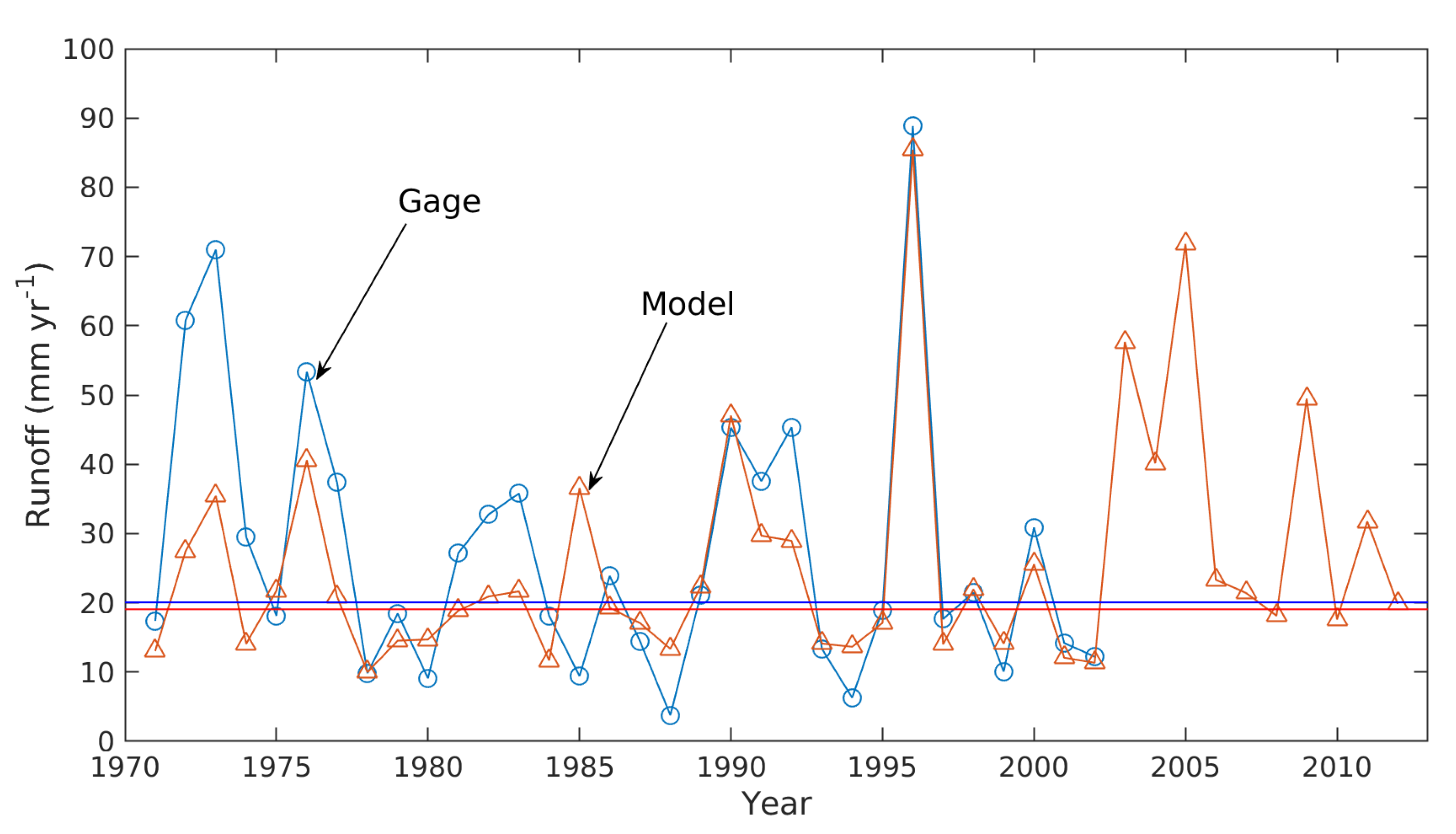
Performance of the WB model on observed climate input, 1969–2012 was checked using gaged Q at Tkabaout, 1971–2002. We allowed two years for the model to stabilize after arbitrary setting of the initial soil-water content for January, 1969, and converted gaged Q to an equivalent average annual depth of runoff, R O * , over the basin for comparison with R O output from the WB model. Modeled R O tracks R O * remarkably well ( r = 0.81 , N = 32 , p < 0.001 ) considering the uncertain quality of the gaged discharge, the estimation of P and T inputs from a sparse network of climate stations, and the use of the default (no tuning) values for parameters of the WB model (Figure 4). The model slightly underestimates median R O * , but the bias is only 5%. The low annual R O * reflects the aridity of the basin: the median annual R O * of 20.1 mm compares with an average grid-cell P of about 367 mm, for an annual R O * /P ratio of 0.055. Neither runoff series plotted in Figure 4 is significantly ( α = 0.05 ) autocorrelated at a lag of one year.
Standard, or default, WB-model parameters [35], as used here, have been found to yield model-output runoff highly correlated with river discharge for basins in diverse climate regimes on several continents [7,12,30]. On the other hand, for basins with long gaged discharge records representative of natural flow, and with corresponding high-quality spatially representative precipitation and temperature time records, it may be advantageous to optimize WB-model parameters to obtain a close match of model-output and gaged runoff. Such an approach has been taken, for example, in WB modeling of the Yellowstone River [6] and Walker River [5] in the western United States.
Water year 1996 is an outlier of high discharge at Tkabaout: R O * in 1996 is more than four times the median for 1971–2002. The WB model strongly corroborates this outlier year of high discharge (Figure 4). Because input P extends through 2012, model-output R O gives some indication of discharge conditions after the record becomes distorted by Koudiet Lamdaouar Dam. Subsequent years of model output show the period 2003–2012 as relatively wet in the basin with a sequence of years, 2003–2005, of high R O and no years of exceptionally low R O .
The WB-model output is consistent with the hydrographs in Figure 2 in pointing to a minor importance of snowmelt to the water balance of the basin. WB-model snowmelt summed for the water year ranges from 3 mm to 64 mm over 1971–2002, and is just 6.4% of the annual P. Local observations also point to snow as an uncommon phenomenon in the study area. Meharzi [45] (translated from French) states that
  • “Snowfall is extremely variable and irregular from one year to another such that high mountain tops are quite often free of snow during almost all of the winter season—as in the winter of 1989–1990, which did not record any days of snow. Quézel [46] reported that the snow season starts by the end of November and continues, depending on the year, until March or April, whenever polar and tropical masses meet during cold periods.”
A short snow record (1979–1988) for Batna indicates that the snowy months there are November–April, with average maximum depth of snow ranging from 2.0 c m in November to 7.8 c m in January. From information in [47], two tree ring fire-history sites near elevation 1900 m located 4 km southeast of the Chemora Basin on Mt. Chélia are characterized by Slimani et al. [48] as having 10–15 snowy days per year and a frost period from November to April with an average of 38 frost days per year.
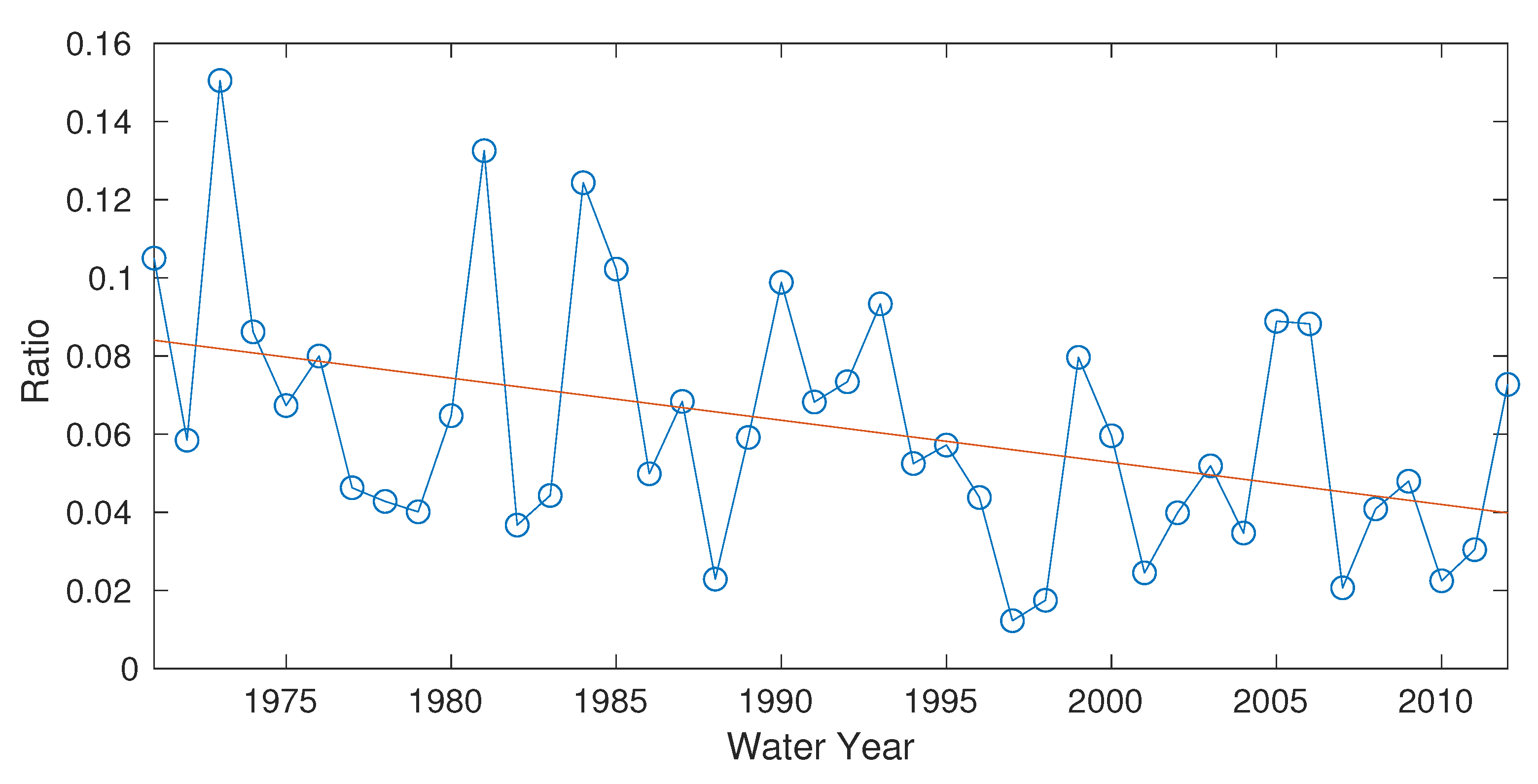
The model-output percentage of P falling as snow declined significantly over 1971–2012 (Figure 5). This decline is likely due to severe warming in the region [49]. The declining snowfall and snowmelt may have a deleterious impact on survival of forests, which are generally at higher elevations, and in this part of North Africa depend strongly on winter and spring moisture [13]. Two episodes of cedar forest decline have been reported in the Aurès and Belezma in the 20th and 21st centuries: the first episode occurred in the late 1970s [50] and affected even the holm oak, which is one of the hardiest species in the region. The second episode was generated by severe droughts that occurred between the end of the 20th and the beginning of the 21st centuries [51,52]. In Belezma, Kherchouche [53] reported that this last episode of dieback started in 2001–2002. These episodes are low points in gage-derived and model-output R O (Figure 4). Declining snowmelt could exacerbate an array of climatic and non-climatic [54] stresses contributing to forest decline here and elsewhere in North Africa.

4.2. Reconstruction Modeling

Principal component analysis (PCA) of the 1853–2005 matrix of 23 standard tree ring chronologies reveals several physically reasonable spatial modes of tree ring variability. Strong common growth patterns over such a widely spaced tree ring network (Figure 1a) are most likely driven by climate. All loadings on PC1 are same-sign, indicating that the primary mode of variation is all chronologies with above normal or below normal growth (Table A1). PC1 explains 41% of the tree ring variance (Table 1). Five PCs have eigenvalues greater than 1, but explained variance drops below 10% after PC3. Accordingly, we retained only PCs 1–3 as potential predictors in subsequent reconstruction modeling.
The loadings on tree ring PC1 and PC2 are mapped in Figure A1, and the loadings for the first three PCs are listed in the last columns of Table A1. We interpret PC1, representing high or low growth across the tree ring network, as a signature of broadly dry or wet conditions over all of northeastern Algeria. PC2 is a north–south contrast, which could reflect a regional gradient in moisture related to storm track location. The loadings could also be interpreted as a species contrast in climate signal, but attribution is conflated by the general north-south stratification of the two tree species (Figure A1). A north–south moisture contrast should be important to Chemora River climate, given the southerly location of the basin within the geographic domain of the tree ring network.
PC3 (not mapped) appears to represent an east–west contrast: negative loadings to the east and positive or near zero loadings to the west (Table A1). An east–west moisture contrast could also be important to Chemora River climate because the basin is toward the eastern part of the tree ring domain. Meharzi [55] highlights the main role of orography in the spatial distribution of rainfall in the Aurès massif and confirms an east–west decreasing gradient. He attributes the wetter conditions in the eastern sector to both elevation, as it is the highest zone of the Aurès, and relief, as the massif is oriented NE–SW, perpendicular to the disturbed northwest flow. Higher order PCs listed in Table 1 become increasingly difficult to interpret in terms of climate because of the orthogonality constraint on PC loadings combined with the decreasing percentage of variance explained.
The regression models described in Section 3.3 for RecD and RecI both use tree ring PCs 1–3 as the pool of potential predictors. The fitted regression equation for the RecD is
y ^ 1 = 0.8326 + 0.0427 x 1 0.0721 x 2
where y ^ 1 is the predicted square root of water-year discharge at Tkabaout (untransformed units m 3 s 1 ), and x i is the score of the ith PC of the 23 standard tree ring chronologies. The fitted regression equation for the RecI reconstruction is
y ^ 2 = 0.9507 + 1.4350 x 1 1.4569 x 2 + 1.0867 x 3
where y ^ 2 is the predicted score of PC1 of annual (water year) P at the 15 precipitation stations in or near the Chemora Basin, and x i is defined as in Equation (3).
The two regression models have roughly similar calibration accuracy and validation skill (Table 2). The adjusted percentage of variance explained by each model for the 1971–2002 calibration period exceeds 65%, and for each model validation RE is only slightly lower than calibration R 2 . Results are consistent with a study of a large network of tree ring chronologies in the western Mediterranean Basin, including our chronologies, that showed a significant positive winter, spring, and summer P signal in P. halepensis and C. atlantica in Algeria, as well as a negative relationship between tree growth and April–August air temperature [13]. The regression coefficient is positive on x 1 and negative on x 2 for both regression models. This is logical considering that a positive loading on tree ring PC1 goes with high growth over the tree ring network and a positive loading on tree ring PC2 goes with a contrast of higher growth in the north of the tree ring network domain and lower growth in the south, where the Chemora Basin is located (Figure 1a). The positive regression coefficient on x 3 in Equation (4) is also physically logical: higher growth (wetter conditions) to the east associated with higher reconstructed Chemora Basin annual P.
The statistics listed in Table 2 for the discharge regression model apply to transformed (square root) annual discharge. In minimizing the sum of squares of transformed discharge, parameter estimates are influenced more by low flows than high flows. The statistics can be misleading as practical measures of reconstruction accuracy because water managers and other users of the data are concerned with accuracy in terms of original units (e.g., m 3 s 1 ). The high R 2 for the annual P reconstruction, while encouraging, does not guarantee that the reconstructed P routed through the WB model will give an accurate reconstruction of Q at the Tkabaout gage. A fair comparison of reconstruction accuracy of RecD and RecI requires additional steps. Back-transforming the predictions from Equation (3) yields RecD, the direct reconstruction of annual Q at Tkabaout in m 3 s 1 . Spatially and temporally disaggregating the predictions from Equation (4) and routing the resulting monthly grid-cell tree ring estimates of P through the WB model yield RecI1 and RecI2, the indirect reconstructions of Q by the alternative methods of temporal disaggregation described in Section 3.3.1. We first discus RecI1, whose temporal disaggregation of reconstructed annual P to monthly P is most straightforward.
Annual Q at Tkabaout, 1971–2002, is tracked more closely by RecD than by RecI1 (Figure 6a). Neither reconstruction preserves the calibration-period mean of observed discharge: the gaged mean for 1971–2001 is 0.68 m 3 s 1 and the reconstructed means for RecD and RecI1 are 0.65 m 3 s 1 and 0.45 m 3 s 1 , respectively. The slight bias in mean for RecD arises because of transformation of the discharge. Preservation of the calibration-period mean of square-root-transformed Q is indeed guaranteed by regression, but this does not hold for Q back-transformed to original units. The larger bias in the mean of RecI1 comes from imperfection in the WB modeling. The interpolation and elevation adjustment of grid-cell P may have resulted in underestimation of grid-cell P. Such an error would transfer to the precipitation PCs and the reconstruction. Moreover, the WB model itself is a simplification of physical processes that operate at finer than grid-cell spatial resolution and shorter than monthly time scales. No WB model can perfectly reproduce discharge from observed P and T, and indeed our model has a slight negative bias with observed P as input (Figure 4). Aside from their offset levels, RecD and RecI1 are similar in their interannual variations, and are highly correlated ( r = 0.90 ) over the 1971–2002 calibration period.
The largest error for both RecD and RecI1 occurs in 1996, which was highlighted earlier as an outlier year of high discharge at Tkabaout. Because the WB Model itself is able to reproduce the high discharge in 1996 from observed monthly P input (Figure 4), the huge RecI1 error in that year is likely due to (1) failure of the tree ring network to capture the magnitude of the annual P anomaly in 1996, or (2) failure of the simplified temporal disaggregation method used in RecI1 to properly apportion the reconstructed annual P to individual months.
WB-model runs on the observed climate input give insight into the unusual hydrology of 1996 and clues to the lack of a commensurate tree ring signal. In the winter of 1996 (DJF, 1995–1996), P was high over the basin, and the greatest P anomalies were at lower elevations toward the northern part of the basin (Figure 7a). Local tree ring sites (those nearest the basin) are at higher elevations, toward the southern end of the basin (Figure 1a). Moreover, despite the high P in 1996, snowfall in DJF was below normal, indicating precipitation as rain rather than snow (Figure 7b). This condition would also oppose a strong tree ring signal, because the P would tend to run off quickly, rather than build a snowpack that gradually melts and reduces drought stress on the trees when they begin growing in spring.
The strong correlation of RecD and RecI1 in the calibration period carries over to common period, 1854–2004, of the long-term reconstructions (Figure 6b,c). Reconstructions are strongly synchronous annually ( r = 0.91 ) and as five-year running means ( r = 0.90 ). The annual time series plots suggest an increase in variability at high frequencies starting about 1960, and a sharp recent trend toward low discharge from 1990 to 2003. RecI1 reaches its lowest annual value in 2001, and lowest five-year moving average in 1999–2003 (Figure 6b,c). This unmatched recent severity of drought is consistent with a regional tree ring reconstruction, 1456–2002 CE, of Palmer Drought Severity Index over Northern Tunisia and Algeria that reaches its lowest five-year moving average in 1998–2002 [24]: the sequence 1998–2002 was the second lowest reconstructed Q in RecI1.
RecD and RecI1 are so similar that they are sometimes indistinguishable on the time series plots (e.g., 1905–1960 in the five-year running mean). The reconstructions occasionally diverge—most notably near 1860 and in the late 1970s—but agree on the timing of most periods of drought and wetness (Figure 6c). It should be noted that series in Figure 6b,c are plotted as z-scores to adjust for the considerably different means and variances of the two reconstructions.
Some similarity in the reconstructions is unavoidable, as both depend, through Equations (3) and (4), on PCs 1 and 2 of the same 23 tree ring chronologies. RecD has the advantage of being “tuned” to observed discharge by regression such that the variance of residuals (observed-reconstructed) of discharge is minimized, though the minimizing is in terms of the square root of discharge rather than of discharge itself. RecI1 is not tuned at all in the calibration process to the gaged discharge. The result is RecI1’s greater bias and lower correlation with observed Q (Figure 6a).
The advantage of RecI1 over RecD is conceptual. Internal water stress in the trees logically responds more directly to precipitation, evaporative stress, and related factors [20] where the trees are growing than to the volume of water passing a stream gage many kilometers away. However, the conceptual advantage in the Chemora Basin is offset by practical limitations. First, our tree ring sites are not distributed over the basin. Unlike a network of rain gages placed strategically to sample P over the important runoff regions of the watershed, our tree ring network is opportunistic: a few sites are on the fringe of the Chemora Basin, and others are hundreds of km away (Figure 1a). Second, disaggregation of annual reconstructed P by constant monthly proportions, as in RecI1, neglects the possible importance to river discharge of variability in the seasonal timing of P. This limitation is addressed with RecI2 later. Third, we assume with the Thornthwaite WB model that a monthly accounting is sufficient for representing the important nonlinear physical processes by which P becomes R O and river discharge. The smaller the basin and the less important snow is to the water balance, the more problematic this assumption.
A fourth limitation of our RecI1 approach is that for this basin we lack tree ring information on the T component of the WB-model input. Tree ring information on interannual variation of T is possible from tree ring wood density in other climate regions [56], but the potential for the Chemora Basin is unknown. On the other hand, the annual P reconstruction (Equation (4)) disaggregated into RecI1 is not strictly “precipitation”: drought-sensitive tree ring chronologies respond to internal water stress in the trees, and this internal water stress is correlated with T. The reconstructed “P” input to the WB model for RecI1 therefore may implicitly include some signal for interannual variation of T. Unalloyed separate reconstructions of P and T may not be attainable with ring widths of drought-sensitive trees.

4.3. Comparative Statistics of RecD and RecI1

Bias in the reconstructions can be summarized by comparing descriptive statistics of observed and reconstructed discharge for the calibration period (Table 3, rows 1–3). The underestimation of median (and mean), more severe in RecI1 than in RecD, has already been discussed. The compression of variance inherent in regression leads to bias toward low standard deviation in both models. Compression of variance in tree ring reconstructions from regression models is a recognized challenge in dendrohydrology that complicates direct comparison of magnitude of events such as droughts in the instrumental and reconstructed record (see, e.g., in [57]).
Like Q for many small streams in semi-arid regions, Q for the Chemora River at Tkabaout is significantly positively skewed. Neither reconstruction effectively captures the skew during the calibration period; skew is positive for both, but not significant. The inability of reconstructions to capture high skew is related to tree ring chronologies being close to normally distributed, and to the tendency for regression-based discharge reconstructions to underestimate the magnitude of discharge in wettest years, as in 1996.
Autocorrelation is an important property of annual discharge because it is associated with duration of droughts and wet periods. The positive and non-significant lag-1 autocorrelation ( r 1 ) of observed Q is close to that of RecI1, but is less than the significant r 1 of RecD (Table 3, rows 1–3, last column). While this could be interpreted as RecD “overstating” the persistence in observed flows, we note that just one year, the outlier high-discharge year 1996, because it is flanked by below-average discharge in 1995 and 1997, has a huge influence on r 1 of observed Q. For example, if observed Q in 1996 were lowered to just 1.22 m 3 s 1 , which is equal to the reconstructed 1996 discharge by RecD (Figure 6a), r1 would increase from r 1 = 0.14 to r 1 = 0.27 and become significant at α = 0.05 .
A long-term context for calibration-period statistics of RecD and RecI1 is given by the statistics for the years prior to the calibration period and for the full-length reconstructions (Table 3, rows 4–7). Reconstructed Q by both RecD and RecI1 was lower, more variable and less autocorrelated in 1971–2002 than in the long-term. RecD, the least biased of the two reconstruction in terms of skew, suggests that the skew of Q for 1971–2002 is representative of long-term skew.
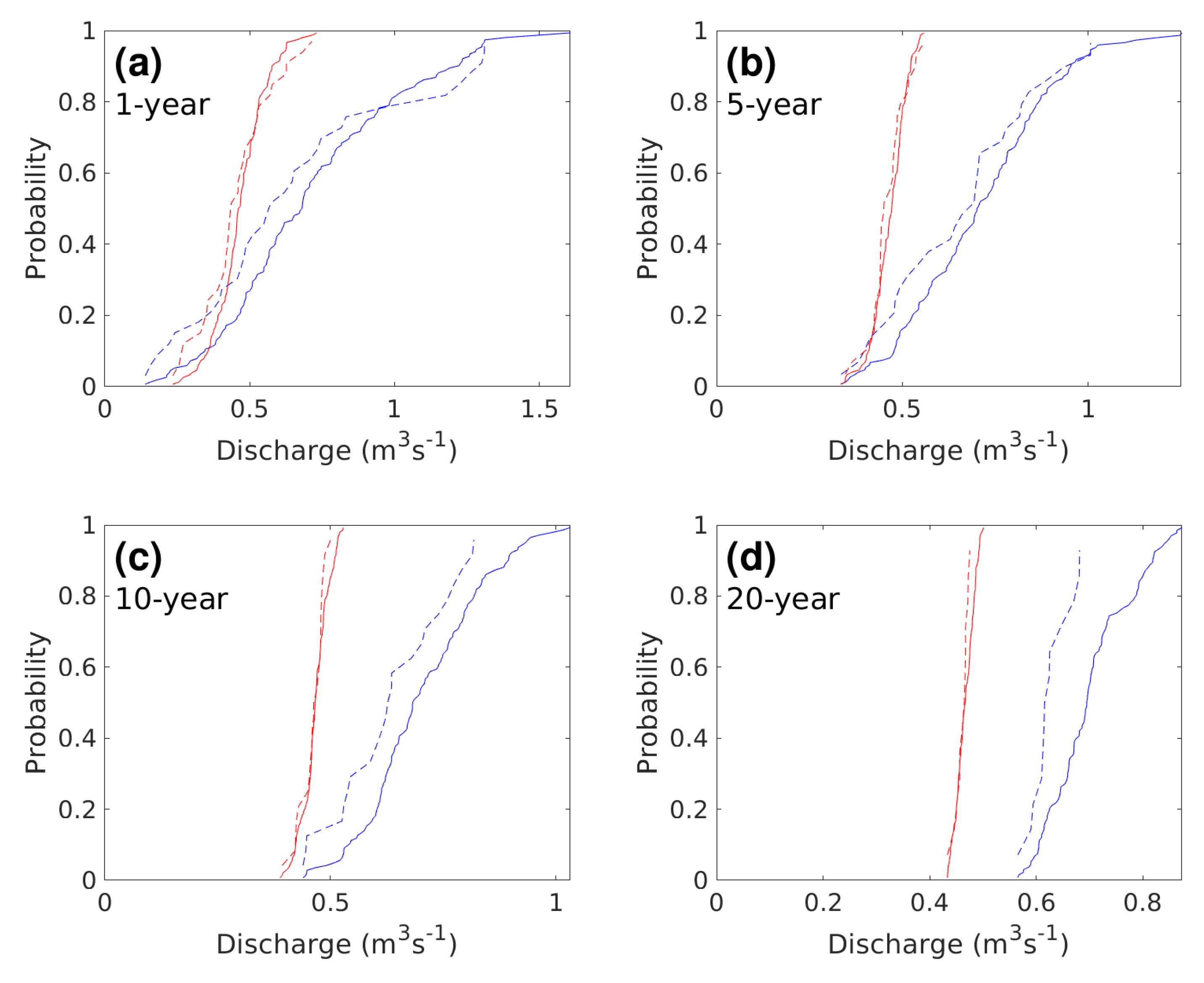
Empirical cumulative distribution functions (CDFs) of reconstructions RecD and RecI1 highlight the large differences in statistical properties of the two reconstructions (Figure 8). To allow assessment of time-dependence of distributions, CDFs are plotted for both the model calibration period (1971–2002) and the full common period of the two reconstructions (1854–2004). CDFs are shown for the annual reconstructions and for three different levels of smoothing. The much greater bias (too low) in median of RecI1 is reflected by the leftward horizontal offset of its CDFs from those of RecD. The compressed x-axis spread of the CDF for RecI1 relative to that of RecD reflects RecI1’s lower explained variance in regression and resulting greater compression of variance. Comparison of the dashed and solid lines for a given model places the distributions for the 1971–2002 calibration period in a long-term perspective. For the unsmoothed reconstructions (Figure 8a), this comparison suggests that the calibration period has been characterized by unusually low and more variable Q. With smoothing, the relatively high variability of reconstructed Q during 1971–2002 disappears (Figure 8b–d). The time series plots of reconstructed Q support the idea that the increased variance or standard deviation of flow during the calibration period is a high-frequency phenomenon (Figure 6b).

4.4. Sensitivity of Reconstruction to Temporal Disaggregation of Annual P

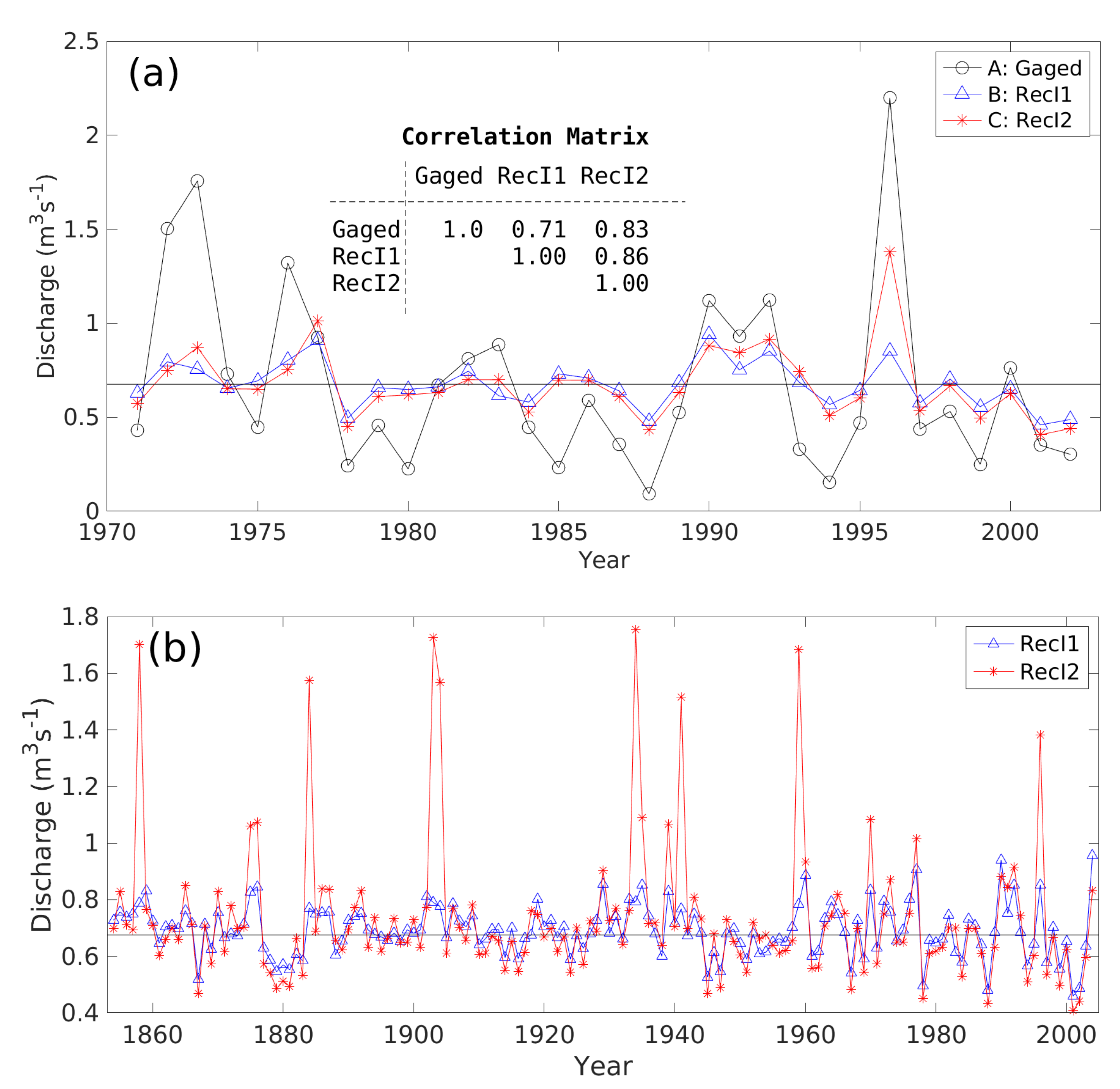
The alternative indirect reconstruction RecI2 was done to check the sensitivity of reconstructed Q to temporal disaggregation—the conversion of reconstructed annual grid-cell P to monthly P. RecI1 keeps the monthly proportions of P constant from year to year, while RecI2 allows the proportions to vary according to the observed proportions in an analog year selected from the 1971–2005 overlap period of the tree ring reconstruction and observed P (Section 3.3.1). For the calibration period, RecI1 and RecI2 are nearly identical, except that RecI2 much more closely tracks the outlier high-discharge year 1996 (Figure 9a). By definition the analog year for reconstruction year 1996 is 1996 itself, so that RecI2 temporally disaggregates reconstructed P according to the actual monthly P proportions in 1996. Clearly the correct specification of the monthly distribution of P is critical for model-output Q to track gaged Q in 1996.
The full-length reconstructions RecI1 and RecI2 agree in most years, but depart radically on average about once a decade, when RecI2 jumps to an extremely high discharge not mirrored by RecI1 (Figure 9b). Because these two reconstructions start with the same reconstructed annual grid-cell P, the only possible source of the huge departures is the apportionment of annual P over months before routing P through the WB Model. The outlier high-Q years result in the long-term mean annual Q from RecI2 being 6% higher than from RecI1. The differences in the two reconstructions underscore the sensitivity of reconstructed Q to the seasonal distribution of annual P.
Could those outlier high-Q years in RecI2 be pre-instrumental analogs to 1996? Moreover, as RecI2 is better than RecI1 at capturing the high discharge in 1996, why not prefer RecI2 to RecI1 as a representation of the long-term discharge history of the Chemora River? We do not argue for accepting reconstruction RecI2 as an accurate representation of the past because the analog-year method used for RecI2 gives hypothetical examples only of possible monthly P proportions over the full reconstruction period. The analog method of temporal disaggregation was found to be inferior to the simple assumption of constant proportions (RecI1) when the two methods were tested in a cross-validation exercise (Appendix A.4; Figure A4). We present RecI2 only to illustrate the possible risk of missing high-discharge years because of the lack of sub-annual resolution of P in the tree rings. A disaggregation approach such as RecI2 might be useful for identifying high-discharge years in reconstructions for other basins if some association between annual P and monthly distribution of P can be demonstrated. Even more useful would be tree ring data with the ability to seasonally resolve precipitation, as has been done in the North American Monsoon region with sub-annual ring-width measurements [58,59] and in other regions with minimum wood density [60]. Both conifer species used here have reasonable color contrast between earlywood and latewood, and would be amenable to partial-width identification and measurement.

4.5. Temporally Variable T

A limitation in our study was the lack of a tree ring proxy for monthly mean T. We dealt with this by assuming that for every year of reconstructions RecI1 and RecI2 monthly mean T was constant at the grid-cell long-term monthly means for the instrumental period. In reality, T varies from year to year and in the Mediterranean Region has been increasing sharply in recent decades [61]. We checked the importance of our T assumption using runs of the WB model on observed monthly P and two alternative settings of monthly T. In one scenario, the input was the observed monthly T. In the other scenario, monthly T was set constant each year at the long-term means for 1971–2002. Results show very little difference in model-output Q for the two T scenarios (Figure A5). Discharge varies much more between the observed gaged Q and model-output Q than between the two versions of model output. The model-output Q by the two assumptions can barely be distinguished in time series plots, and are almost perfectly correlated ( r = 0.99 ). Discharge is probably insensitive to interannual variations in T in the Chemora Basin because the P that contributes most to runoff and discharge comes mainly in the winter, when T, P E T and A E T are low. We conclude that the lack of a tree ring T proxy is not critical to indirect reconstruction of Q in the Chemora Basin, and is less important than the lack of seasonally resolved P.

5. Conclusions

This study demonstrates the value of WB modeling and the potential of indirect reconstruction for unraveling the pre-instrumental history of river discharge from total-width tree ring chronologies in a small semi-arid watershed. The direct and indirect reconstruction methods both give statistically significant reconstructions of discharge of the Chemora River that correlate strongly at high and low frequencies. Accuracy is greater for the direct reconstruction, but the WB modeling associated with the indirect reconstruction helps explain large reconstruction errors in both reconstructions. Results suggest that severe underestimation of discharge in the high-flow year 1996 could stem from a combination of circumstances: mismatch of locations of tree ring sites and P anomalies, monthly timing of P that cannot be deciphered with the tree ring data, and unusually low snow/precipitation ratio in that particular year.
The WB-model run on observed monthly P and T input indicates that the snow fraction of P in the basin is decreasing over time. Despite the typically small contribution of snowmelt to the water balance of this basin, forest sustainability could suffer from this trend because forests are primarily located at the higher elevations, where snowpack is deepest.
The two versions of indirect reconstruction (RecI1 and RecI2) explored here both relied on temporal disaggregation of reconstructed annual P to provide the monthly P input to a WB model. Our results strongly suggest that proper apportioning of reconstructed annual P to months is critical to capturing the magnitude of extreme high-discharge years on the Chemora River. RecI1, with constant monthly proportions, likely misses occasional high-discharge years such as 1996 in the long-term tree ring record. RecI2, with analog-year proportions, gives occasional occurrences of high-discharge years. Despite deficiencies in our particular analog method, it highlights the need for tree ring estimates of P at higher than annual resolution for improved indirect discharge reconstruction.
WB modeling with observed T and invariable (year-to-year) T suggests that runoff and river discharge in the Chemora Basin are relatively insensitive to interannual variability of T. This is probably due to the aridity of the basin, the winter dominance of P and the relatively low importance of snowmelt to the water balance. Accordingly, the potential gain in accuracy of reconstruction of discharge from a tree ring proxy for T is probably much less than the gain from improved tree ring resolution of seasonal P.
Small river basins, such as the Chemora Basin, are especially challenging for discharge reconstruction from tree rings because high flows, especially, can be generated by localized storm systems that might not be sampled by a widely dispersed tree ring network. The challenge is magnified when large P events are rain rather than snow, as P can run off quickly and generate huge flows without leaving a commensurate footprint in the soil moisture sensed by trees. Although we point out some severe shortcomings of the indirect reconstruction method for this particular basin, we underscore the value of the WB modeling itself as diagnostic tool in error analysis and in assessing amenability of a small basin to discharge reconstruction for tree rings.

Author Contributions

D.M.M., conceptualization, software development, data analysis, original draft preparation, and funding acquisition; R.T., field collections, tree ring chronology development, review and editing, data archiving, and funding acquisition; D.K., field collections, tree ring measurement, acquisition of local hydrologic data, and review and editing; S.S., field collections, and review and editing. All authors have read and agreed to the published version of the manuscript.

Funding

This research was funded by National Science Foundation Awards 0317288, 1103314 and 1903535.

Acknowledgments

We wish to thank our colleagues and various institutions from Algeria: Abdallatif Gasmi and Messaoud Hamidi (Conservators of the Forests of Batna and Khenchela, respectively); Athmane Briki (Batna Forest Department) for making this study possible; the National Agency of Water Resources, Algeria, for providing us with streamflow and precipitation data; and the National Office of Meteorology, Algeria for providing the climate data of Batna station. We thank Christopher Baisan and Alexis Arizpe for their valuable assistance in the field. We thank Jim Burns for his help in dating the tree ring sites. We thank the numerous student workers who have assisted in sample preparation.

Conflicts of Interest

The authors declare no conflict of interest.

Abbreviations

The following abbreviations are used in this manuscript.
A E T Actual evapotranspiration
CDFCumulative distribution function
GHCNGlobal Historical Climate Network
PPrecipitation
P C Principal component
P C A Principal component analysis
P E T Potential evapotranspiration
QRiver discharge (e.g., in  m 3 s 1 )
RecDDirect reconstruction
RecIIndirect reconstruction ( in general)
RecI1Indirect reconstruction with constant (year-to-year) monthly proportion of annual P
RecI2Indirect reconstruction with variable (year-to-year) monthly proportion of annual P
R O Runoff
SSoil water storage
Δ S Change in soil water storage
TAir temperature
WB modelWater-balance model

Appendix A

Appendix A.1. Statistics of Tree Ring Site Chronologies

This appendix includes additional information on the tree ring data. Tree ring chronologies, tree species, site coordinates, and descriptive statistics for the 23 standard tree ring chronologies used in this study are listed in Table A1. The measured ring widths are available from Dr. Ramzi Touchan. The loading patterns for the first two principal components of the chronologies are mapped in Figure A1.
Chronology development was not part of this paper. The following quote from [25] summarizes salient points of standardization, which was accomplished with program ARSTAN [21]:
  • A uniform and systematic procedure was applied in chronology development. Each series of tree ring width measurements was fit with a cubic smoothing spline with a 50% frequency response at 67% of the series length to remove non-climatic trends due to age, size, and the effects of stand dynamics [62]. The detrended series were then prewhitened with low-order autoregressive models to remove persistence not related to climatic variations. The individual indices were combined into a single master chronology for each combination of site and species using a bi-weight robust estimate of the mean [63]. The adequacy of sample replication was judged by the expressed population signal (EPS), computed from pooled interseries correlations and the time-varying sample size [23].
Table A1. Tree ring chronology statistics a .
NIDSpecies b LatLongElev (m)Years c PC1 d PC2PC3
1AEHCEAT35.336.9017561607–2012 (1607)0.21850.00070.3258
2BORCEAT35.596.0418761148–2011 (1733)0.23080.0204−0.0185
3DJTCEAT36.454.1014601534–2011 (1725)0.12060.39340.0031
4FERCEAT35.386.9615221384–2011 (1672)0.25540.01070.2045
5IGICEAT36.474.0014431621–2005 (1845)0.18930.3090−0.0959
6KERCEAT36.422.8913981849–2011 (1913)0.08510.2862−0.0257
7KESCEAT35.852.0015601717–2006 (1819)0.16410.1698−0.2941
8LMOCEAT36.454.1115181697–2005 (1894)0.12420.39740.0564
9OUTCEAT35.316.6320731002–2011 (1480)0.21570.01420.2283
10PIPCEAT35.851.9814521533–2012 (1854)0.18170.0376−0.3265
11TAGCEAT35.176.1517041814–2012 (1821)0.2340−0.12800.0799
12THTCEAT36.474.0215501747–2005 (1878)0.11920.38010.0024
13TIGCEAT36.454.1016971552–2011 (1741)0.09740.4037−0.0157
14TIZCEAT35.306.6319701344–2011 (1445)0.2111−0.05030.2809
15TUGCEAT35.576.0416741732–2009 (1737)0.2722−0.07310.1346
16AKSPIHA35.286.6614131851–2011 (1857)0.2337−0.12820.2514
17ALKPIHA34.552.8013571853–2011 (1866)0.2464−0.1007−0.2572
18BOCPIHA35.136.6212731695–2011 (1756)0.2196−0.07990.2016
19DJEPIHA35.216.4713031834–2011 (1850)0.2183−0.11020.2404
20FEBPIHA34.562.7813341794–2011 (1833)0.2419−0.1561−0.2601
21THNPIHA34.613.0913861830–2011 (1861)0.2542−0.1100−0.2613
22TOBPIHA34.623.1313311851–2011 (1855)0.2365−0.2144−0.2583
23ZEBPIHA34.533.0114151835–2011 (1848)0.2586−0.1403−0.2435
a Site number, site code, species code, latitude, longitude, elevation (m), time coverage, and loadings of first three principal components (PCs). b Species code: CEAT = Cedrus atlantica, PIHA = Pinus halepensis. c First and last year of chronology, followed by (in parentheses) first year the expressed population signal [23] exceeds 0.85. d PC1, PC2, and PC3 are loadings of first three PCs from PCA of the 1853–2005 time series matrix of standard chronologies. Note: Ramzi Touchan has subsequently incorporated additional samples into seven site chronologies, resulting in the following current start and end years for those sites: AEH 1070–2012; BOR 1147–2011]; KES 1717–2011; LMO 1697–2011; OUT 1002–2014; TAG 1814–2014; TIZ 912–2011. Moreover, three-character codes have changed for four sites in Touchan’s current database (new codes in parentheses): FER (TIA); PIP (PEP); TIZ (THZ); TUG (AIK).
Figure A1. Tree ring chronology loading patterns on first two principal components of site chronologies. (a) First principal component, or PC1. (b) Second principal component, or PC2. The principal component analysis (PCA) was run on the 1853–2005 matrix of 23 standard chronologies using the correlation matrix. Pinus halepensis are circles, Cedrus atlantica are triangles. Negative weights are blue and positive weights are red. Largest and smallest symbols on each map correspond to highest and lowest absolute loadings. Size of symbol is proportional to size of loading. Plotting coordinates have been dithered slightly on the map to enable distinguishing sites located very close to one another.
Forests 11 00986 g0a1

Appendix A.2. Water-Balance Modeling

This appendix includes additional details on the WB modeling and a sketch of the WB model (Figure A2). Fortran code for the WB model was obtained from Greg McCabe (U.S. Geological Survey; personal communication), and was adapted to run on a laptop under a Linux (Ubuntu) operating system using the gfortran-4.9.1 Fortran compiler. The model, represented by the sketch in Figure A2, runs at a monthly time step and requires as time series input monthly total precipitation (P) and monthly mean temperature (T). These inputs had to be estimated for the grid cells of the model from station climate data, as described in the main paper and expanded on in Appendix A.3. The model equations are presented elsewhere [35] and are not repeated here. We used the default program settings of model parameters. In the interest of reproducibility, we list below our specific settings of model parameters. For ease of reference, we use the same abbreviations for water balance terms as in [35].
  • w h c = 150 mm; water holding capacity of the soil (soil moisture storage capacity).
    Any excess of soil moisture storage, S, above w h c in the monthly accounting is allocated to runoff ( R O ). In running the model, it is necessary to assume an S at the beginning of the first month of available P and T. Because this initial value is unknown, the WB output for some time can be distorted by incorrect specification of initial S. This is typically handled by disregarding the first year or two of model outputs. Our modeling, for example, on observed data, begins with January of 1969. We assume initial saturation ( S = 150 mm), and we do not start interpreting the WB-model outputs until water year 1971 (defined as October 1970 to September 1971). If w h c is exceeded, the excess is “surplus.”
  • t s n o w = 4.0 ° C ; T threshold for snow. Below this threshold of monthly mean T all P is snow, or P s n o w .
  • t r a i n = 7.0 ° C T threshold for rain. Above this threshold of monthly mean T all P is rain, or P r a i n . Between a monthly mean T of t r a i n and t s n o w , the fraction of P as P r a i n varies linearly in proportion to the fraction ( T t s n o w ) / ( t r a i n t s n o w ) .
  • d i r e c t f a c = 0.05 ; decimal fraction of P r a i n to direct runoff. This small fraction of total P r a i n is assumed to immediately (same month) contribute to direct R O rather than to enter into the water balance of the soil column, no matter how dry that soil is.
  • r f a c t o r = 0.50 ; runoff factor. The decimal fraction of surplus assigned to R O . This surplus, as defined above, is not all assigned to R O in the same month, but is gradually released according to this rule.
  • x m e l t c o e f f = 0.47 ; daily melt coefficient. This coefficient along with the difference T T s n o w determines what fracton of the snow water storage is assigned to snowmelt runoff in the month. (Notation here is taken from the Fortran program rather than [35].) The snowmelt is computed as x m e l t = x m e l t c o e f f ( T T s n o w ) N , where N is the number of days in the month. This equation can yield an x m e l t greater than the actual snow water storage, and in that case the entire snowpack is assumed to melt (i.e., x m e l t cannot exceed the existing snow water storage).
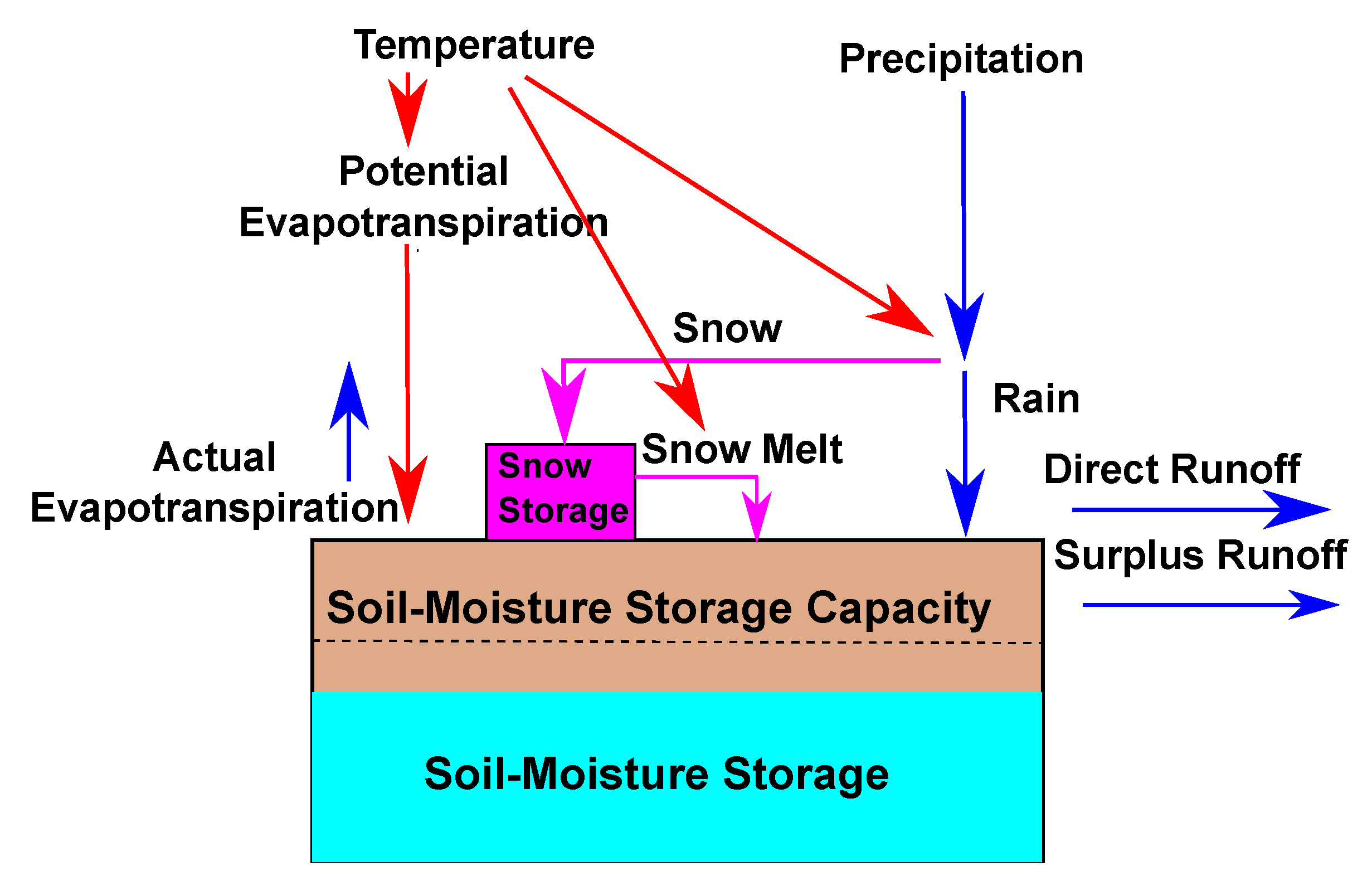
Figure A2. Simplified sketch of water balance model. Figure adapted from [35].
Forests 11 00986 g0a2

Appendix A.3. Grid-Cell Monthly P and T from Station Data

This appendix gives additional details on the conversion of observed station monthly P and T to the grid-cell observed monthly P and T required as input to the WB model.
Precipitation. Station P with almost complete coverage for 1969–2012 at 15 stations in or near the basin was first converted to standardized monthly anomalies using the station monthly means and standard deviations for 1969–2012. The standardized anomalies were then interpolated to the 154 grid-cell centers by inverse distance weighting [36] using the five stations nearest the center of the grid cell. To avoid excessively high weights on stations that happen to be near the centers of the grid cells, any station-cell distance less than 3 km was set to 3 km before the weighting.
To convert interpolated standardized anomalies to units of P (mm), it was necessary to multiply each standardized anomaly for year i and month j by an appropriate monthly standard deviation and then add an appropriate monthly mean. Because of the strong importance of elevation to mean P in the region, and a positive relationship of standard deviation and mean, we used regression of 1969–2012 station monthly means and coefficients of variation of P on elevation to estimate the appropriate grid-cell monthly means and standard deviations. Steps, repeated for each month of year, are: (1) regress station long-term (1969–2012) mean monthly P on station elevation and substitute grid-cell central elevation into the regression to get the estimated grid-cell mean, (2) repeat the regression using the coefficient of variation instead of the mean as the predictand to get an estimated grid-cell coefficient of variation of P, (3) compute the grid-cell standard deviation as the product of the grid-cell monthly mean and the monthly coefficient of variation, and (4) multiply the standardized anomaly in each year by the standard deviation and add back the mean to get grid-cell P in mm. This procedure, repeated for all months of the year and grid cells, yields a continuous time series matrix of “observed” monthly P, 1969–2012, at each of the 154 grid cells.
Temperature. The procedure to generate the 1969–2012 input of monthly observed T for the water-balance modeling differed from the procedure for P in two main ways. It was first necessary to estimate some missing monthly T at Batna1, and for this we used linear regression of the monthly T at Batna1 on the monthly T at nearby station Batna2, which is serially complete for 1950–2012. Because anomalies of monthly T are generally highly spatially coherent, and because we had just one reasonably long monthly adjusted Global Historical Climate Network (GHCN) T series (Batna1) near the study basin (Figure 1a), we assumed that apart from scaling of mean and variance to deal with elevation differences the Batna1 inter-annual T variations are representative of the entire Chemora Basin. Accordingly we assumed the monthly standardized T anomaly at Batna1 applies to each of the 154 grid cells.
The resulting standardized anomalies of monthly T at the 154 grid cells—identical for each cell—were then converted to units of ° C using monthly means and standard deviations appropriate for the grid cells. Monthly means for grid cells were estimated by adjusting the Batna1 monthly means for elevation using a seasonally varying lapse rate and the elevation difference at Batna1 and the grid-cell center. Following [38], we assumed the following seasonally varying lapse rate ( ° C   k m 1 ) for months January-December: 4.5, 5.0, 6.0, 6.3, 6.4, 6.5, 6.5, 6.5, 6.2, 5.5, 5.0, 4.5.
The standard deviation of monthly grid-cell T for a given grid cell and month was estimated as as the product of the long-term monthly mean T estimated from the lapse rate, and the long-term monthly coefficient of variation of T estimated by regression of coefficients of variation of T against station elevation for the six Algeria GHCN stations on the map in Figure 1a. The analysis period for the regressions was 1969–2015. The GHCN stations had considerable missing data; the regression model for a given month was estimated using only those years with data for the month at all stations; this sample size varied from 30 to 34 years.

Appendix A.4. Indirect Reconstruction Modeling

This appendix gives additional details on indirect reconstruction as implemented in the paper. Supplemental figures are also presented to illustrate the identification of analog years for the temporal disaggregation for RecI2 (Figure A3), to summarize results of a cross-validation check of the analog method of temporal disaggregation (Figure A4), and to demonstrate the low sensitivity of annual discharge in this basin to the inter-annual variation of T (Figure A5).
The starting point for the steps outlined here is the n 1 × p matrix P of annual (water-year) P for n 1 = 43 years 1970–2012 at the p = 91 Chemora Basin grid cells. As described in the paper, the grid-cell P was interpolated from station P. Our indirect reconstruction procedure has a series of sequential objectives. A first objective is grid-cell reconstructed annual P for the n 2 = 153 years 1853–2005, the common period of the 23 available tree ring chronologies. A second objective is to convert the reconstructed grid-cell P into calendar-year monthly grid-cell P to be input into the WB model. The approach to these objectives is broadly to reconstruct the first principal component (PC1) of annual P using tree rings, and to disaggregate that reconstructed time series spatially to grid cells and temporally to the 12 months of the water year. The statistical part of the reconstruction is regression of the precipitation PC1 on principal components (PCs) of tree ring chronologies using a calibration period of n 3 = 32 years, 1971–2002. This period was selected because it is the same calibration period, dictated by the usable gaged Q record, used for the direct reconstruction.
Steps in Indirect Reconstruction. The procedure is described here with matrix algebra, beginning with P , the n 1 × p time series matrix of annual (water year) P for the n 1 = 43 water years 1970–2012 at p = 91 Chemora Basin grid cells.
  • Convert P to standardized anomalies, Z , using the 1970–2012 column means and standard deviations, and store the column-wise statistics in column vectors x ¯ and s .
  • PCA on Z to get: V , a p × p matrix of principal component (PC) loadings and F , a n 1 × p time series matrix of PC scores.
  • Regress first column of F (scores of first precipitation PC) on tree ring variables in stepwise regression using a calibration period of n 3 = 32 years, 1971–2002; this calibration period was selected to match the calibration period for direct reconstruction, and so is limited by the usable part of the discharge record at Tkabaout.
  • Apply the estimated regression equation to get reconstructed F 1 ^ for the n 2 = 153 years 1853–2005, where the ^ refers to “predicted”, and the subscript “1” refers to the first component.
  • Spatially disaggregate F 1 ^ to get reconstruction annual z-scores of P at the 91 grid cells: Z ^ = F 1 ^ V 1 T , where T denotes transpose and V 1 is the first column of the principal components matrix, V .
  • Restore grid-cell means and standard deviations to convert Z ^ to annual (water year) reconstructed grid-cell P in units of mm: P ^ = Z ^ D + 1 x ¯ , where D is a diagonal matrix with elements of s along the diagonal, and 1 is a column vector of ones of length n 2 .
  • Temporally disaggregate the n 2 × p time series matrix P ^ , as described in the main paper, to derive the reconstructed monthly grid-cell P needed as input to the WB model.
  • Route the resulting monthly P, and assumed monthly time series of grid-cell T through the WB model to come up with estimated monthly grid-cell runoff ( R O ), 1854–2004. For the indirect reconstructions in this study we used long-term monthly mean observed T, invariable from year to year. Water balance modeling was applied to roughly assess how sensitive discharge in this basin is to the interannual variability of T (see main paper, and Figure A5). The different spans, 1853–2005 vs 1854–2004, of the tree ring coverage and the WB-model output water year totals (e.g., R O ) are due to (1) loss of leading year to allow spin-up of WB model from initial conditions and (2) loss of trailing year in reorganizing water-year (October-September) monthly data from the temporal disaggregation into water-year monthly input required by the WB model.
  • Convert grid-cell estimated R O to monthly, seasonal or annual discharge at the Tkabaout gage by multiplying R O (a depth of water) by grid-cell area, and integrating over cells and months.
Identifying Analog Years. Analog years were used in reconstruction version RecI2 (see main paper) to specify how reconstructed grid-cell annual (water year) P is apportioned to individual months of the water year. This procedure is called temporal disaggregation. Let F ^ t be the reconstructed scores of the first principal component (PC) of Chemora Basin (91 grid cells) annual (water year) P, 1853–2005. As described in the paper the reconstruction was done by regression using a calibration period of water years 1971–2002. The analog year for a reconstructed F ^ t 0 in year t = t 0 was defined as the year in the interval 1971–2005 with reconstructed F t closest to F ^ t 0 . The monthly proportions of observed P in that analog year were then assigned to the reconstructed annual grid-cell P in year t 0 . By this method, each reconstruction year maps to an analog year in 1971–2005. The mapping is illustrated in Figure A3, where reconstruction year 1867 maps to 1978. A reconstructed water year P in 1867 would then be apportioned over months in the same proportions as the observed P in 1978. By this algorithm, the reconstruction F ^ t for any year in the interval 1971 t 2002 maps to the year t 0 (e.g., reconstruction year 1975 maps to 1975). In other words, for any year of the 1971–2002 calibration period, reconstructed annual P is allocated to months in exactly the same proportions as observed P for that same year.
Cross-validation of Analog Years An ad-hoc cross-validation method was used to check whether the analog method just described is better than the long-term-mean proportions as an estimator of the proportion of P in the 12 months (Oct-Sept) of the water year. The cross-validation test uses observed grid-cell monthly P for the 43 water years 1970–2012. For each of the 91 grid cells, there is a time series vector, p , of annual (water year) P, 1970–2012, and a corresponding matrix of monthly values, P .
  • Choose one of the 91 grid cells.
  • Drop 1970 (first year) from the vector of annual values and matrix of monthly values.
  • Assign as the analog year the year in the interval 1971–2012 with closest annual P to that in 1970.
  • Compute Spearman correlation coefficient between the 12-element vector of monthly P proportions in 1970 and in the analog year.
  • Compute Spearman correlation coefficient between the 12-element vector of monthly P proportions in 1970 and the vector of long-term-mean proportions for 1971–2012.
  • The method giving the highest correlation is judged “best” for that year (1970).
  • Repeat steps 2–6 for all years 1970–2012, each time leaving out one year and using the remaining 42 years for getting the “predicted” proportions. This process results in two sets of 43 Spearman correlations—one set with the monthly proportions in the analog-year as the predictor, the other set with the long-term-mean monthly proportions as the predictor.
  • Plot the histograms of the correlations for this grid cell (e.g., Figure A4, for grid cell #84—a representative higher-elevation gridpoint).
  • Repeat 1–8 for all gridpoints. This gives 91 pairs of distributions of correlation cofficients for each of the two disaggregation methods being compared. Results are summarized in the caption to Figure A4.
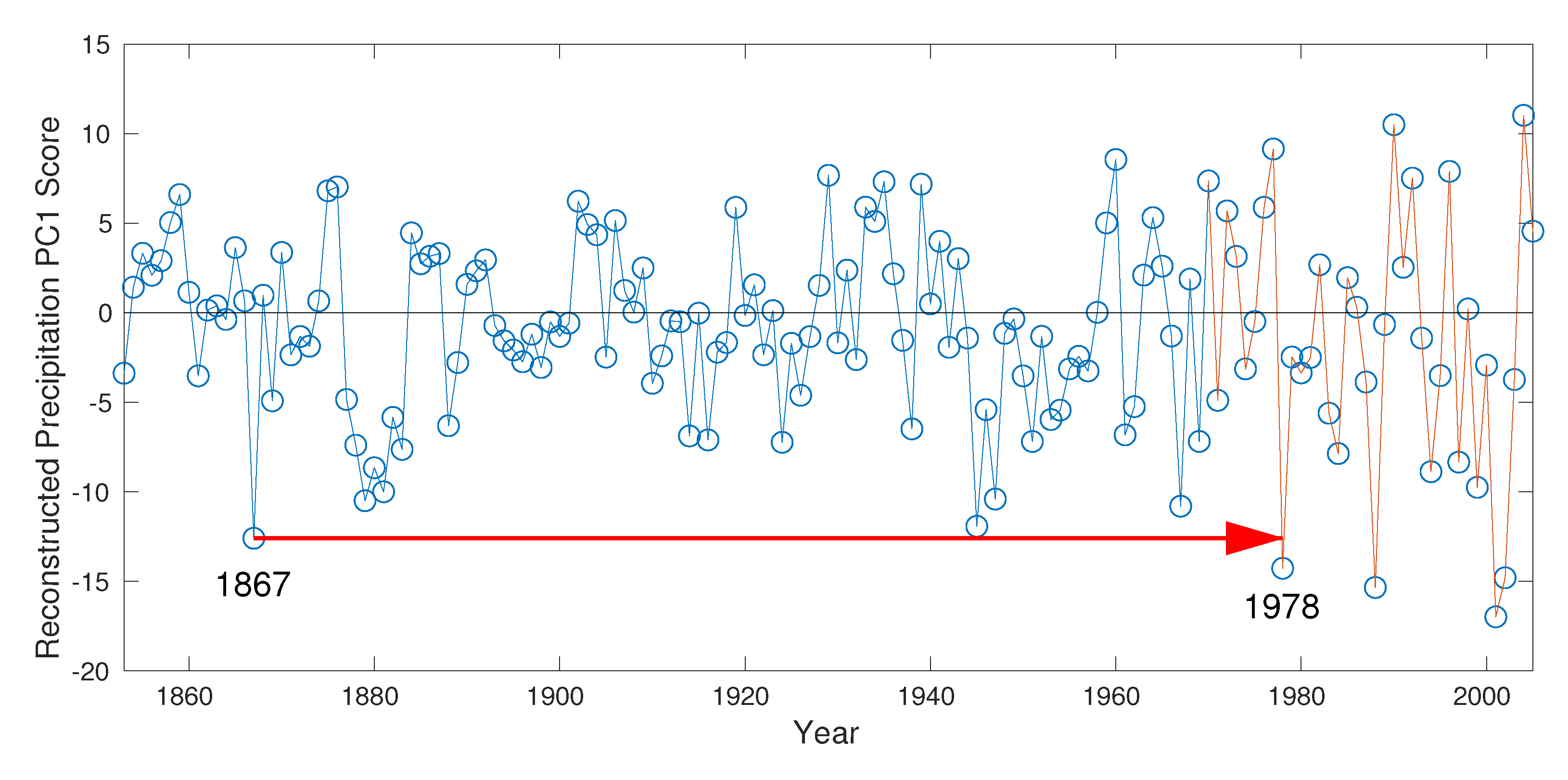
Figure A3. Time plot of precipitation reconstruction illustrating assignment of analog year. Plotted variable is the dimensionless reconstructed score of the first principal component of z-score transformed P, 1853–2005. Analog year is defined as the reconstructed value in the interval 1970–2005 (the overlap of observed and reconstructed P) closest to that in the reconstruction year. For example, reconstruction year 1867 maps to calibration-period year 1978.
Forests 11 00986 g0a3
Figure A4. Analog-year cross-validation for gridpoint #84. Histograms of Spearman rank correlations of predicted with observed 12-element vectors of monthly proportions of annual water-year P in target years by two alternative predictions. Each histogram represents 43 correlations—one for each year in the interval 1970–2012. (a) Analog year as predictor. (b) Long-term-mean proportions as predictor. Similar plots can be made for each of the 91 grid cells in the Chemora Basin. For all cells, the median of the 43 correlations was higher for long-term-means predictor than for the analog predictor. We conclude that the total annual P is inferior to the long-term-mean proportions as a predictor of the proportion of P in the 12 months of the water year.
Forests 11 00986 g0a4
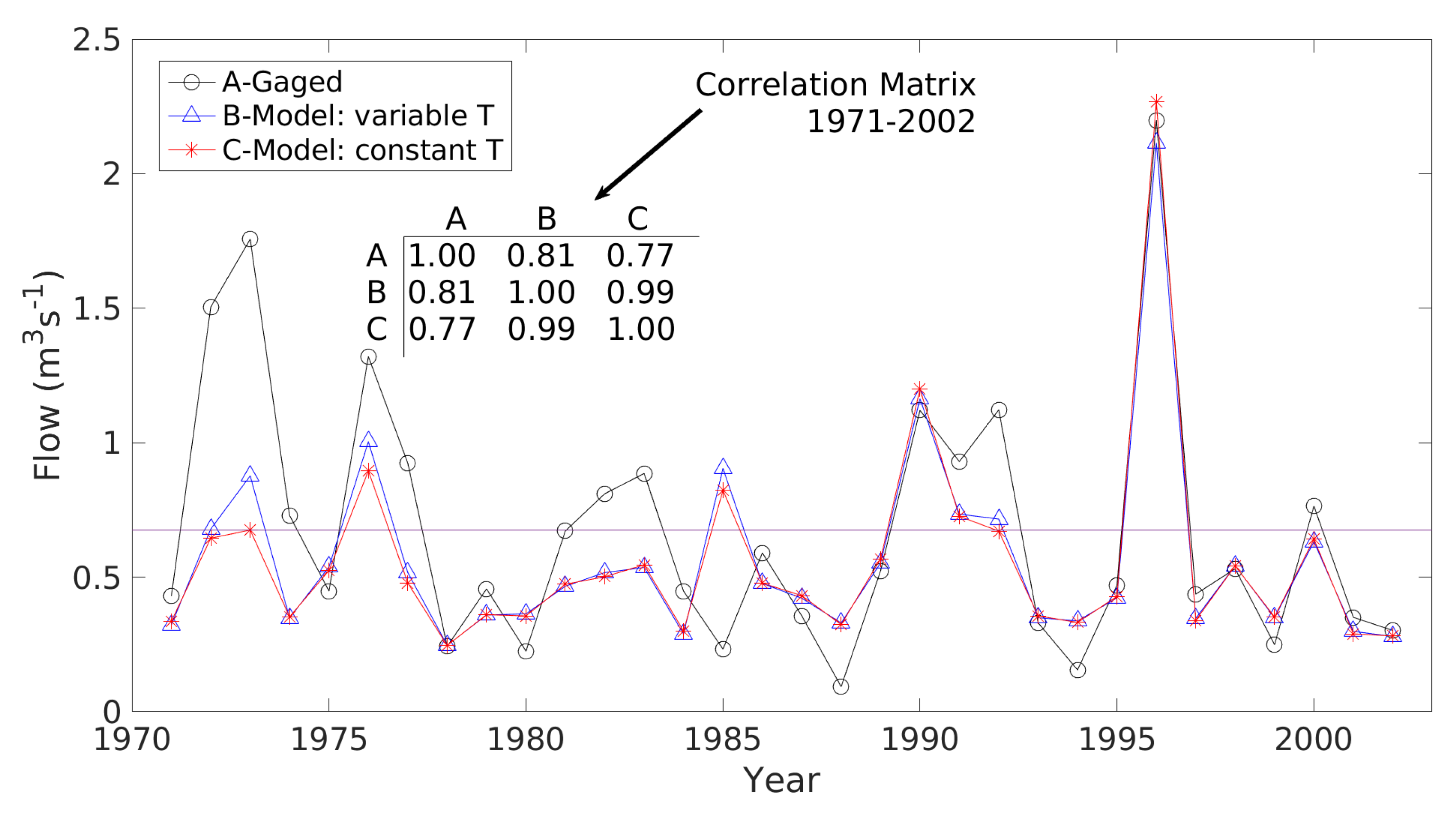
Sensitivity of Model-Output Discharge to Inter-Annual Variability of Temperature. As described in the main paper, the importance of variable (year-to-year) T to discharge (Q) was checked by running the WB model twice, both times using the observed monthly grid-cell P but with alternative assumptions about monthly grid-cell T: (1) using observed grid-cell monthly T, and (2) setting grid-cell monthly T each year at the 1971–2002 long-term grid-cell monthly means. Resulting WB-model output Q for those two assumptions is compared to the observed Q in Figure A5.
Figure A5. Time series plots of gaged Q and model-output Q from WB model using variable and constant T. For series B, monthly T is set to the observed grid-cell T, which varies from year to year. For series C, monthly T is set at the long-term monthly means for 1971–2002, and is the same each year. Model runs for (B) and (C) used the same monthly P input, set to the observed grid-cell P. Correlation matrix of the three series annotated.
Forests 11 00986 g0a5

References

  1. Loaiciga, H.A.; Haston, L.; Michaelsen, J. Dendrohydrology and long-term hydrologic phenomena. Rev. Geophys. 1993, 31, 151–171. [Google Scholar] [CrossRef]
  2. Meko, D.M.; Woodhouse, C.A. Application of Streamflow Reconstruction to Water Resources Management. In Dendroclimatology, Progress and Prospects; Hughes, M.K., Swetnam, T.W., Diaz, H.F., Eds.; Developments in Paleoenvironmental Research; Springer: Dordrecht, The Netherlands, 2011; Volume 11, pp. 231–261. [Google Scholar]
  3. Graham, N.E.; Hughes, M.K. Reconstructing the Mediaeval low stands of Mono Lake, Sierra Nevada, California, USA. Holocene 2007, 17, 1197–1210. [Google Scholar] [CrossRef]
  4. Saito, L.; Biondi, F.; Salas, J.D.; Panorska, A.K.; Kozubowski, T.J. A watershed modeling approach to streamflow reconstruction from tree ring records. Environ. Res. Lett. 2008, 3. [Google Scholar] [CrossRef]
  5. Saito, L.; Biondi, F.; Devkota, R.; Vittori, J.; Salas, J.D. A water balance approach for reconstructing streamflow using tree ring proxy records. J. Hydrol. 2015, 529, 535–547. [Google Scholar] [CrossRef] [Green Version]
  6. Gray, S.T.; McCabe, G.J. A combined water balance and tree ring approach to understanding the potential hydrologic effects of climate change in the central Rocky Mountain region. Water Resour. Res. 2014, 46, W05513. [Google Scholar] [CrossRef]
  7. Gangopadhyay, S.; McCabe, G.J.; Woodhouse, C.A. Beyond annual streamflow reconstructions for the Upper Colorado River Basin: A paleo-water-balance approach. Water Resour. Res. 2015, 51, 9763–9774. [Google Scholar] [CrossRef] [Green Version]
  8. Cleaveland, M.K. A 963-year reconstruction of summer (JJA) stream flow in the White River, Arkansas, USA, from tree rings. Holocene 2000, 10, 33–41. [Google Scholar] [CrossRef]
  9. Meko, D.M.; Woodhouse, C.A.; Baisan, C.H.; Knight, T.; Lukas, J.J.; Hughes, M.K.; Salzer, M.W. Medieval drought in the Upper Colorado River Basin. Geophys. Res. Lett. 2007, 34. [Google Scholar] [CrossRef] [Green Version]
  10. Cook, E.R.; Palmer, J.G.; Ahmed, M.; Woodhouse, C.A.; Fenwick, P.; Zafar, M.U.; Wahab, M.; Khan, N. Five centuries of Upper Indus River flow from tree rings. J. Hydrol. 2013, 486, 365–375. [Google Scholar] [CrossRef] [Green Version]
  11. Biondi, F.; Meko, D.M. Long-term hydroclimatic patterns in the Truckee-Carson Basin of the eastern Sierra Nevada, USA. Water Resour. Res. 2019, 55, 5559–5574. [Google Scholar] [CrossRef] [Green Version]
  12. McCabe, G.J.; Wolock, D.M. Joint variability of global runoff and global sea-surface temperatures. J. Hydrometeorol. 2008, 9, 816–824. [Google Scholar] [CrossRef]
  13. Touchan, R.; Anchukaitis, K.J.; Meko, D.M.; Kerchouche, D.; Slimani, S.; Ilmen, R.; Hasnaoui, F.; Guibal, F.; Camarero, J.J.; Sánchez-Salguero, R.; et al. Climate controls on tree growth in the Western Mediterranean. Holocene 2017, 27, 1429–1442. [Google Scholar] [CrossRef]
  14. Guidoum, A.; Nemouchi, A.; Hamlat, A. Modeling and mapping of water erosion in northeastern Algeria using a seasonal multicriteria approach. Arab. J. Geosci. 2014, 7, 3925–3943. [Google Scholar] [CrossRef]
  15. Tiri, A.; Lahbari, N.; Boudoukha, A. Assessment of the quality of water by hierarchical cluster and variance analyses of the Koudiat Medouar Watershed, East Algeria. Appl. Water Sci. 2017, 7, 4197–4206. [Google Scholar] [CrossRef] [Green Version]
  16. Berghout, A.; Meddi, M. Sediment transport modeling in Wadi chemora during flood flow events. J. Water Land Dev. 2016, 31, 23–31. [Google Scholar] [CrossRef]
  17. Trouet, V.; van Oldenborgh, G. KNMI Climate Explorer: A web-based research tool for high-resolution paleoclimatology. Tree Ring Res. 2013, 69, 3–13. [Google Scholar] [CrossRef] [Green Version]
  18. Sharples, J.J.; Hutchinson, M.F.; Jellett, D.R. On the horizontal scale of elevation dependence of Australian monthly precipitation. J. Appl. Meteorol. 2007, 44, 1850–1865. [Google Scholar] [CrossRef]
  19. NCEI. 2-Minute Gridded Global Relief Data (ETOPO2v2). 2020. Available online: https://www.ngdc.noaa.gov/mgg/global/etopo2.html (accessed on 13 August 2015).
  20. Fritts, H.C. Tree Rings and Climate; Academic Press: London, UK, 1976; 567p. [Google Scholar]
  21. Cook, E.R.; Krusic, P.J.; Holmes, R.H.; Peters, K. Program ARSTAN, Version 41d. 2007. Available online: www.ldeo.columbia.edu/tree-ring-laboratory (accessed on 10 August 2020).
  22. Cook, E.R.; Kairiukstis, L.A. (Eds.) Methods of Dendrochronology: Applications in the Environmental Sciences; Kluwer Academic Publishers: Dordrecht, The Netherlands, 1990; 394p. [Google Scholar]
  23. Wigley, T.M.L.; Briffa, K.R.; Jones, P.D. On the average value of correlated time series, with applications in dendroclimatology and hydrometeorology. J. Clim. Appl. Meteor. 1984, 23, 201–213. [Google Scholar] [CrossRef]
  24. Touchan, R.; Anchukaitis, K.J.; Meko, D.M.; Attalah, S.; Baisan, C.; Aloui, A. Long term context for recent drought in northwestern Africa. Geophys. Res. Lett. 2008, 35, L13705. [Google Scholar] [CrossRef]
  25. Touchan, R.; Anchukaitis, K.; Meko, D.M.; Sabir, M.; Attalah, S. Spatiotemporal drought variability in northwestern Africa over the last nine centuries. Clim. Dynam. 2011, 37, 237–252. [Google Scholar] [CrossRef]
  26. Mardia, K.; Kent, J.; Bibby, J. Multivariate Analysis; Academic Press: London, UK, 1979; 518p. [Google Scholar]
  27. Thornthwaite, C.W. An approach toward a rational classification of climate. Geog. Rev. 1948, 38, 55–94. [Google Scholar] [CrossRef]
  28. Thornthwaite, C.W.; Mather, J.R. The Water Balance: Publications in Climatology; Technical Report; Drexel Institute of Technology: Philadelphia, PA, USA, 1955; Volume 1, 144p. [Google Scholar]
  29. McCabe, G.J.; Wolock, D.M. Warming may create substantial water supply shortages in the Colorado River basin. Geophys. Res. Lett. 2007, 34. [Google Scholar] [CrossRef] [Green Version]
  30. McCabe, G.J.; Wolock, D.M. Century–scale variability in global annual runoff examined using a water balance model. Int. J. Climatol. 2011, 31, 1739–1748. [Google Scholar] [CrossRef]
  31. Palmer, W.C. Meteorological Drought, Research Paper No. 54; Technical Report; NOAA: Washington, DC, USA, 1965; 58p. Available online: https://www.ncdc.noaa.gov/temp-and-precip/drought/historical-palmers/overview (accessed on 18 July 2020).
  32. Stockton, C.W.; Meko, D.M. A long-term history of drought occurrence in western United States as inferred from tree rings. Weatherwise 1975, 28, 244–249. [Google Scholar] [CrossRef]
  33. Cook, E.R.; Meko, D.M.; Stahle, D.W.; Cleaveland, M.K. Drought reconstructions for the continental United States. J. Climate 1999, 12, 1145–1162. [Google Scholar] [CrossRef] [Green Version]
  34. Hamon, W.R. Estimating potential evapotranspiration. J. Hydraul. Div. 1961, 87, 107–120. [Google Scholar]
  35. McCabe, G.J.; Markstrom, S.L. A Monthly Water-Balance Model Driven by a Graphical User Interface; Open-File Report 2007-1088; U.S. Geological Survey: Reston, VA, USA, 2007; 6p.
  36. Jones, P.D.; Hulme, M. Calculating regional climate time series for temperature and precipitation: Methods and illustrations. Int. J. Climatol. 1996, 16, 3. [Google Scholar] [CrossRef]
  37. Haan, C.T. Statistical Methods in Hydrology, 2nd ed.; Iowa State University Press: Iowa City, IA, USA, 2002; 496p. [Google Scholar]
  38. Barry, R.G. (Ed.) Mountain Weather and Climate, 3rd ed.; Cambridge University Press: London, UK, 2008; 506p. [Google Scholar]
  39. Weisberg, S. Applied Linear Regression, 2nd ed.; John Wiley: New York, NY, USA, 1985; 324p. [Google Scholar]
  40. Michaelsen, J. Cross-validation in statistical climate forecast models. J. Clim. Appl. Meteor. 1987, 26, 1589–1600. [Google Scholar] [CrossRef] [Green Version]
  41. Fritts, H.C.; Guiot, J.; Gordon, G.A. Verification. In Methods of Dendrochronology: Applications in the Environmental Sciences; Cook, E.R., Kairiukstis, L.A., Eds.; Kluwer Academic Publishers: New York, NY, USA, 1990; pp. 178–185. [Google Scholar]
  42. Woodhouse, C.A.; Gray, S.T.; Meko, D.M. Updated streamflow reconstructions for the Upper Colorado River Basin. Water Resour. Res. 2006, 42. [Google Scholar] [CrossRef]
  43. Hidalgo, H.G.; Piechota, T.C.; Dracup, J.A. Alternative principal components regression procedures for dendrohydrologic reconstructions. Water Resour. Res. 2000, 36, 3241–3249. [Google Scholar] [CrossRef] [Green Version]
  44. Snedecor, G.W.; Cochran, W.G. Statistical Methods, 8th ed.; Iowa State University Press: Ames, IA, USA, 1989; 503p. [Google Scholar]
  45. Meharzi, M.K.E. Forêts, Géosystèmes et Dynamique du Milieu: Le cas de l’Aurès. Ph.D. Thesis, Université des frères Mentouri Constantine, Constantine, Algeria, 2010. [Google Scholar]
  46. Quézel, P. Peuplement Végétal des Hautes Montagnes de l’Afrique du Nord. Essai de Synthèse Biogéographique et Phytosociologique; Lahure, A., Ed.; Éditions Paul Lechevalier: Paris, France, 1957; 463p. [Google Scholar]
  47. Belloula, N. Etude expérimentale de l’Influence de la typologie des Cédraies sur la distribution des formes d’Azote dans certains sols du massif forestier du Chélia (W. de Khenchela). In Mémoire de Magister; Université Hadj Lakhdar Batna: Batna, Algeria, 2011; 136p. [Google Scholar]
  48. Slimani, S.; Touchan, R.; Derridj, A.; Kherchouche, D.; Gutiérrez, E. Fire history of Atlas cedar (Cedrus atlantica Manetti) in Mount Chélia, Northern Algeria. J. Arid Environ. 2014, 104, 116–124. [Google Scholar] [CrossRef]
  49. Seager, R.; Liu, H.; Henderson, N.; Simpson, I.; Kelley, C.; Shaw, T.; Kushnir, Y.; Ting, M. Causes of increasing aridification of the Mediterranean region in response to rising greenhouse gases. J. Clim. 2014, 27, 4655–4676. [Google Scholar] [CrossRef] [Green Version]
  50. Abdessemed, K. Le cèdre de l’Atlas (Cedrus atlantica Man.) dans les Massifs de l’Aurès et du Belezma: Etude Phytosociologique, Problèmes de Conservation D’aménagement. Ph.D. Thesis, Université de Droit d’Economie et des Sciences d’Aix-Marseille, Aix-en-Provence, France, 1981. [Google Scholar]
  51. Bentouati, A.; Bariteau, M. Réflexions sur le dépérissement du cèdre de l’Atlas des Aurés (Algérie). Forêt Méditerranéenne 2006, XXVII, 317–322. [Google Scholar]
  52. Kherchouche, D.; Kalla, M.; Gutierrez, E.; Attallah, S.; Bouzghaia, M. Impacts of droughts on Cedrus atlantica forests dieback in the Aurés (Algeria). J. Life Sci. 2012, 6, 1262–1269. [Google Scholar]
  53. Kherchouche, D.; Kalla, M.; Gutierrez, E.; Briki, A.; Hamchi, A. La sécheresse et le dépérissement du cèdre de l’Atlas (Cedrus atlantica Manetti) dans le massif du Belezma (Algérie). J. Life Sci. 2013, 24, 129–137. [Google Scholar]
  54. Moon, H.; Solomon, T. Forest decline in Africa: Trends and impacts of foreign direct investment: A review. Int. J. Curr. Adv. Res. 2018, 7. [Google Scholar] [CrossRef]
  55. Meharzi, M.K. Le rôle de l’orographie dans la répartition spatiale des précipitations dans le massif de l’Aurès. Méditerranée 1994, 3, 73–78. [Google Scholar] [CrossRef]
  56. Björklund, J.; Gunnarson, B.E.; Seftigen, K.; Zhang, P.; Linderholm, H.W. Using adjusted Blue Intensity data to attain high-quality summer temperature information: A case study from Central Scandinavian. Holocene 2015, 25, 547–556. [Google Scholar] [CrossRef]
  57. Robeson, S.M.; Maxwell, J.T.; Ficklin, D.L. Bias correction of paleoclimatic reconstructions: A new look at 1200+ years of Upper Colorado River flow. Geophys. Res. Lett. 2020, 47, e2019GL086689. [Google Scholar] [CrossRef]
  58. Griffin, D.; Woodhouse, C.A.; Meko, D.M.; Stahe, D.W.; Faulstich, H.L.; Carillo, C.; Touchan, R.; Castro, C.; Leavitt, S. North American monsoon precipitation reconstructed from tree ring latewood. Geophys. Res. Lett. 2013, 40, 1–5. [Google Scholar] [CrossRef]
  59. Woodhouse, C.A.; Meko, D.M.; Griffin, D.; Castro, C.L. Tree rings reveal multi-season drought variability in the lower Rio Grande basin, USA. Water Resour. Res. 2013, 49, 844–850. [Google Scholar] [CrossRef]
  60. Camarero, J.; Fernández-Pérez, L.; Kirdyanov, A.V.; Shestakova, T.A.; Knorre, A.A.; Kukarskih, V.V.; Voltas, J. Minimum wood density of conifers portrays changes in early season precipitation at dry and cold Eurasian regions. Trees 2017, 31, 1423–1437. [Google Scholar] [CrossRef] [Green Version]
  61. Lionello, P.; Scarascia, L. The relation between climate change in the Mediterranean region and global warming. Reg. Environ. Chang. 2018, 18, 1481–1493. [Google Scholar] [CrossRef]
  62. Cook, E.R.; Briffa, K.; Shiyatov, S.; Mazepa, V. Tree ring standardization and growth-trend estimation. In Methods of Dendrochronology: Applications in the Environmental Sciences; Kluwer Academic Publishers: Dordrecht, The Netherlands, 1990; pp. 104–123. 394p. [Google Scholar]
  63. Cook, E.R. A Time Series Approach to Tree Ring Standardization. Ph.D. Thesis, The University of Arizona, Tucson, AZ, USA, 1985. [Google Scholar]
Figure 1. Data locations and study basin. (a) Small scale map with tree ring sites, climate stations, and Chemora River Basin (gray patch). Tree ring sites are green triangles (15 Cedrus atlantica) and green circles (8 Pinus halepensis). Climate stations are squares: black for 15 P stations and red for 6 T stations. Population centers Algiers and Batna are asterisks. Inset map at lower right shows location of study region within Mediterranean Basin. (b) Digital elevation model (DEM) for 2 × 2 grid including the Chemora Basin (solid red outline). The water-balance modeling domain includes 154 cells, 91 of which are at least partly in the Chemora Basin.
Forests 11 00986 g001
Figure 2. Monthly hydrographs for key Chemora River stations. (a) Mean monthly precipitation at station Ain Tinn. (b) Gaged discharge of Chemora River at Tkabaout. Ain Tinn (35.378 ° N, 6.439 ° E, 1650 m) is the highest elevation precipitation station in the 15-station network used to develop the water-balance model input. Analysis period for hydrographs is 1970–2002.
Forests 11 00986 g002
Figure 3. Schematic contrasting direct and indirect reconstruction methods. At the start, Q t is gaged discharge, X is a time series matrix of principal components (PCs) of tree ring chronologies, F t is the first PC of annual (water year) P at a network of stations, and T ¯ j , k is long-term monthly mean T for month j, grid-cell k. Regression and reconstruction yield predicted quantities ( ^ ). For the indirect method, a reconstruction, F ^ t , of the first PC of annual P is disagreggated spatially to grid cells and then temporally to months to get the required P input for the WB model. Model output runoff is summed over cells in the river basin to get Q ^ t . For the direct method, Q ^ t is estimated by the more straightforward process of regression of gaged Q on tree ring PCs (see text).
Forests 11 00986 g003
Figure 4. Time plots of annual runoff as gaged and as output by WB model. The two series correlate highly ( r = 0.81 ) over their 1971–2002 common period. Median annual runoff (horizontal lines) for that common period is 20.1 m m (gage) and 19.1 m m (model).
Forests 11 00986 g004
Figure 5. Declining ratio of water-year snowmelt to P. The negative-slope straight line is from a linear regression of R a t i o against year, where R a t i o is the ratio of water-year (October-September) WB-model output snowmelt to water-year total P averaged over the 91 model grid cells in the Chemora River Basin. The estimated regression equation is R a t i o ^ = 2.2083 0.00108 t , where t is the year and R a t i o ^ is the estimated ratio. The regression, fit to years 1971–2012, explains 17% of the variance of R a t i o and is statistically significant (F = 8.2801, p = 0.0.0064).
Forests 11 00986 g005
Figure 6. Discharge reconstructed directly and indirectly. (a) Annual (Oct–Sept) discharge of Chemora River as measured at Tkabaout gage and as reconstructed directly (RecD) and indirectly (RecI1) from tree rings. Series plotted for 1971–2002 calibration period of the reconstructions. Horizontal line at gaged mean. Correlation matrix annotated. (b) Annual reconstructions, 1854–2004, of discharge by models RecD and RecI1. (c) Five-year running mean of annual reconstructions, plotted at fifth year. Reconstructed series in panels (b,c) converted to zero mean and unit standard deviation before plotting. Correlation coefficients are 0.91 for the two reconstructed annual series in panel (b) and 0.90 for the smoothed series in panel (c).
Forests 11 00986 g006
Figure 7. Water-balance model precipitation and snowfall over Chemora Basin in winter of 1995–1996. (a) Precipitation. (b) Snowfall. The mapped quantity is percentage of normal, defined as the grid-cell mean for 1971–2002. Winter is DJF.
Forests 11 00986 g007
Figure 8. Empirical cumulative distribution functions (CDFs) of reconstructed discharge. Probability of non-exceedance is plotted against reconstructed discharge. Panels (ad) show for CDFs different levels of smoothing of the annual series, as annotated at upper left. Curves for RecD (blue) and RecI1 (red) are shown for the 1971–2002 calibration period (dashed) and the full-length (1854–2004) reconstruction (solid). Smoothing is by running means.
Forests 11 00986 g008
Figure 9. Sensitivity of indirect reconstruction to monthly distribution of annual P. (a) Calibration- period discharge as gaged, and as reconstructed indirectly with alternative assumptions about the monthly distribution of P. RecI1 assumes a constant distribution equal to the average monthly mean proportions for 1971–2002. RecI2 uses the observed monthly proportion of P, which varies from year to year. Horizontal line is gaged mean for 1971–2002. Series RecI1 and RecI2 have been shifted before plotting such that means for 1971–2002 identical to that of gaged flow. Before shift, the means of series A, B, and C are 0.675, 0.450, and 0.501 m 3 / s , respectively. Correlations between time series for 1971–2002 are annotated. (b) Long-term reconstructions by RecI1 and RecI2. For RecI2, the annual reconstructed P in any year is assumed to be distributed over months the same as in an identified “analog” year in the interval 1971–2002 (see text).
Forests 11 00986 g009
Table 1. Principal component analysis a of tree ring chronologies.
PC λ PctgInterpretation
19.33740.6Common growth signal; all loadings positive
23.30314.4Species contrast or north-south contrast
32.32110.1East-west contrast
41.6917.4Remaining components have no clear interpretation
51.0054.4
60.8793.8
a Component number followed by eigenvalue, percentage of variance explained, and interpretation.
Table 2. Reconstruction model statistics a .
PredictandStepsPCs Entered R 2 RE
Discharge b 21, 20.650.59
Precipitation c 31, 3, 20.680.63
a Number of regression steps, tree ring PCs in model, adjusted R 2 , and reduction of error statistic; PCs entered listed in order of entry in stepwise regression; calibration period 1971–2002. b Discharge (water year) of Chemora River at Tkabaout. c PC1 of time series matrix of annual P for the 91 Chemora Basin grid cells.
Table 3. Descriptive statistics a of gaged discharge and reconstructions for different intervals.
YearsStatistics
Segment b SeriesFirstLastMeanMedianStd c Skewr1
Calib. PeriodGaged197120020.6760.4970.4881.39 *0.14
RecD197120020.6510.5660.3600.580.33 *
RecI1197120020.4500.4340.1200.230.13
EarlierRecD185419700.7260.6850.2900.59 *0.44 *
RecI1185419700.4700.4680.0770.010.29 *
FullRecD185420040.7120.6800.3090.53 *0.39 *
RecI1185420040.4670.4600.0900.130.20 *
a Mean, median, standard deviation (std), skewness coefficient (skew), and lag-1 autocorrelation (r1); units for first three are m 3 s 1 . b Period for statistics, defined by first and last year. c Asterisk for std and r1 indicated significance at α = 0.05 .