Using GatorEye UAV-Borne LiDAR to Quantify the Spatial and Temporal Effects of a Prescribed Fire on Understory Height and Biomass in a Pine Savanna

Abstract

In the pine savannas of the southeastern United States, prescribed fire is commonly used to manipulate understory structure and composition. Understory characteristics have traditionally been monitored with field sampling; however, remote sensing could provide rapid, spatially explicit monitoring of understory dynamics. We contrasted pre- vs. post-fire understory characteristics collected with fixed area plots with estimates from high-density LiDAR point clouds collected using the unmanned aerial vehicle (UAV)-borne GatorEye system. Measuring within 1 × 1 m field plots (n = 20), we found average understory height ranged from 0.17–1.26 m and biomass from 0.26–4.86 Mg C ha⁻¹ before the fire (May 2018), and five months after the fire (November 2018), height ranged from 0.11–1.09 m and biomass from 0.04–3.03 Mg C ha⁻¹. Understory heights estimated with LiDAR were significantly correlated with plot height measurements (R² = 0.576, p ≤ 0.001). Understory biomass was correlated with in situ heights (R² = 0.579, p ≤ 0.001) and LiDAR heights (R² = 0.507, p ≤ 0.001). The biomass estimates made with either height measurement did not differ for the measurement plots (p = 0.263). However, for the larger research area, the understory biomass estimated with the LiDAR indicated a smaller difference after the burn (~12.7% biomass reduction) than observed with in situ measurements (~16% biomass reduction). The two approaches likely differed because the research area’s spatial variability was not captured by the in-situ measurements (0.2% of the research area measured) versus the wall-to-wall coverage provided by LiDAR. The additional benefit of having spatially explicit measurements with LiDAR, and its ease of use, make it a promising tool for land managers wanting greater spatial and temporal resolution in tracking understory biomass and its response to prescribed fire.

1. Introduction

In the southeastern United States, the forested landscape was once dominated by longleaf pine (Pinus palustris Mill.) stands, mixed stands of longleaf pine, and slash pine (Pinus elliottii Engelm.), or mixed stands of longleaf with other species [1]. Mature forests featuring these species associations once covered 37 million ha [1,2], but longleaf pine in particular declined by nearly 98% due to logging, fire suppression, conversion to agricultural and other land uses, and replacement by other types of forests [3,4,5,6,7]. This reduction of native longleaf pine savannas coincided with the decline of more than 30 native plants and animal species, making them threatened or endangered [2,8]. Restoring these pine ecosystems has become a regional priority for public and private entities as a way to maintain biodiversity and increase forest functional diversity [5].

A key component of restoring the region’s pine savanna ecosystems is allowing fire to periodically affect the development of the understory. During the precolonial era, wildfire is estimated to have burned vast areas, often as groundfires that recurred at 1–10 year intervals [1]. Fire typically has a minimal effect on mature pine trees, as many species in the region have bark characteristics that protect against groundfires. However, as seedlings, both longleaf pine and slash pine are intolerant to competition for light, making their natural regeneration dependent on some repression of competing vegetation with fire [9]. With the region-wide suppression of wildfire, land managers now need to use prescribed fire to alter understory biomass and encourage pine regeneration [10]. Thus, knowing the spatial distribution of understory biomass before a fire [11], and the resulting response of understory plants to the prescribed fire [12] could benefit restoration objectives. However, conducting this type of survey of the understory with clipped plots is labor-intensive, and as a result, the provided information is generally limited in spatial and temporal extent.

Acquiring high-spatial-resolution LiDAR data in an ecosystem managed with prescribed fire can help fire managers to quickly estimate the amount of understory-related fuel load [13,14], the location of dense biomass accumulation [15,16,17,18], and the biomass consumed by fire [19,20], thereby allowing them to better manage the severity of the fire and to customize prescribed fire treatments for preferred ecological benefits [21,22]. The accuracy of LiDAR estimates of understory height and biomass has varied across studies [23,24,25,26]. Understory with low stature is often difficult to measure using airborne LiDAR as a laser pulse may fail to hit the ground point, or miss the highest point of sparse understory vegetation, thus underestimating shrub height [26]. Increasing laser pulse density can overcome this issue, but the lower economic importance of understory species relative to trees may reduce interest in increasing point density [27], which may increase measurement time or the subsequent processing time needed to extract understory variables.

High-density point sampling can be achieved with LiDAR mounted on a piloted aircraft; however, flight time scheduling, cost, and the repeat passes often necessary for high point density from aircraft can preclude data collection using these platforms. In contrast, LiDAR sensors mounted on an unmanned aerial vehicle (UAV) can gather understory and ground information with scans at a much higher point-density than piloted aircraft because UAVs can often fly at lower altitudes and slower than piloted fixed-wing aircraft [28,29]. In addition, UAV systems usually have lower costs per flight and allow for more flexible flying schedules than aircraft [30]. Flexibility may be a key feature for making LiDAR useful in prescribed fire applications, as rapid deployment could make it more likely that an assessment of understory conditions occurs before or after the expected timing of a burn. UAV LiDAR technology has been shown to provide spatially explicit estimates of aboveground tree biomass [31]; however, few studies have focused on forest understory biomass using UAVs.

In the lower coastal plain of the southeastern United States, the ‘flatwood’ pine savannas are ecosystems found near coastal or poor drainage areas where periodic flooding occurs [32]. The mesic to hydric soil conditions and aggressive understory growth make these pine savanna’s particularly challenging to manage with prescribed fire. Here small wetland depressions are scattered among well- to poorly-drained soils, creating notable spatial variation in both soil moisture and the amount of understory biomass [33]. The resulting variation in fuel loads, moisture, and post-fire understory recovery can create uncertainty in prescribed fire behavior and in quantitatively assessing whether management goals are met with an applied fire. The objective of this study was to understand how understory structure, specifically height and biomass, varied spatially before and after a fire in a pine savanna. The study used clipped plot biomass harvests coupled to UAV collected LiDAR point clouds, both of which were collected at approximately the same time during two different periods: (1) before the burn and (2) five months after the burn, to investigate the spatial and temporal influence of prescribed fire on understory structure.

2. Materials and Methods

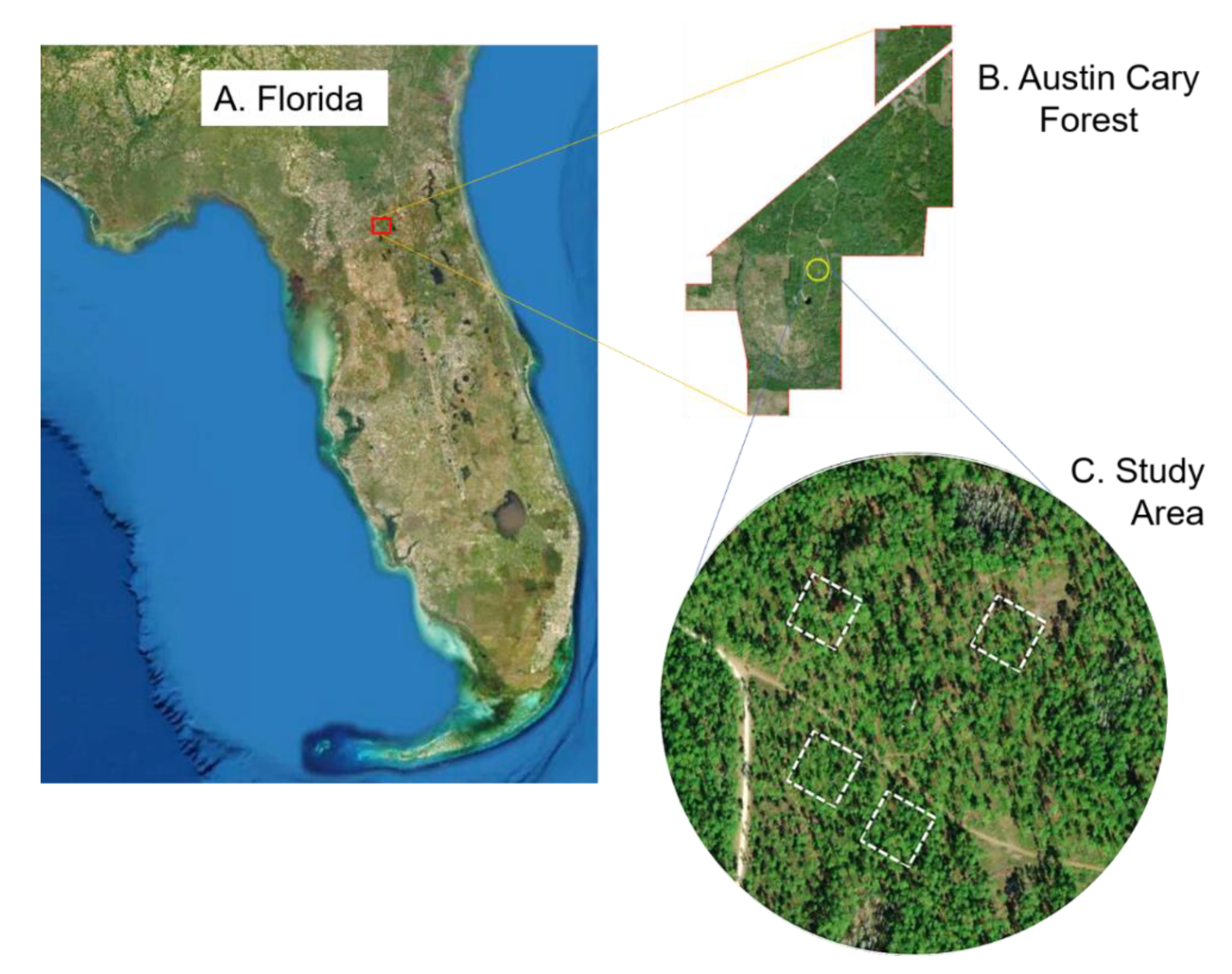
2.1. Site Description

The study was conducted in north-central Florida, about 15 km northeast of Gainesville, at the Austin Cary Forest (ACF), managed by the University of Florida (Figure 1). The study site included four 50 × 50 m permanent plots inside the forest that were established in 1999 and were randomly located within an eddy-covariance tower’s footprint [33]. The study area was a mixed stand of naturally regenerated longleaf pine (~70% of trees) and slash pine (~30% of trees). In 2018, the research area had a density of 185 trees per ha⁻¹ with an average tree diameter of 30.31 ± 6.66 cm, basal area of 13.61 ± 0.03 m² ha⁻¹, and height of 22.47 ± 6.33 m. Because the overstory canopy was relatively open, the understory was dense and mostly dominated by saw palmetto (Serenoa repens (W. Bartram) Small), gallberry (Ilex coriacea (Pursh) Chapm), and wax myrtle (Myrica cerifera (L.) Small) [34]. The trees in the plots were approximately 80-year-old, where the approximate age of longleaf pine was 90 years, and that of slash pine was 70 years. The soil was mostly acidic, Ultic Alaquods (sandy, siliceous, thermic), poorly drained, and low in organic matter. Two of the four measurement areas were located in a wetter area of the site, while the other two were located in a drier area (Figure 1).

The region had seasonal precipitation with long-term mean annual precipitation of 1219 ± 218 mm (1988–2018) [35] and a long-term mean annual temperature of 20.77 °C (1988–2018) [35]. The average minimum and maximum monthly air temperature ranged from 12.8 °C in January to 27.5 °C in July [35].

The ongoing management objective for this forest is to restore and maintain an uneven-aged, old-growth savanna-like pine forest with a widely spaced overstory and a diverse understory species composition. Thinning and a three-year prescribed fire cycle have been used to achieve these management objectives. Selective thinning was done in May 2016, where approximately 30% of the trees per ha were harvested, of which ~70% were longleaf pine, and ~30% were slash pine. The first prescribed burn was done at the time of the plot establishment in 2000. Since then, the area was burned every three years (2003, 2006, 2009, 2012, 2015, and 2018). The most recent prescribed burn was conducted in June 2018. These burns, on average, were of moderate intensities with flame heights reaching no more than 1.5 m, with burns carefully monitored by fire crews (S. Sager, Austin Cary Forest, Gainesville, FL, USA, personal communication).

2.2. Field Data Collection

We measured understory heights and biomass before the prescribed burn (May 2018) ~one week after (June 2018), and then again five months (November 2018), and one year (June 2019) after the burn. We collected understory metrics on five 1 × 1 m subplots inside four 50 × 50 m permanent plots (20 subplots total) (Figure 1c). Plots were located with randomly generated numbers to assign the location of each understory subplot both before and after the burn. In each subplot, we measured the height of the understory using two levels of point density: (1) in the measurement before the burn, we measured the heights at four plot corners and at the center (five points total), (2) after the burn, we measured the heights in a grid at 25 cm apart in the x-axis and 10 cm apart in the y-axis, resulting in 55 points in total in each subplot. We changed the point sampling density because, before the burn, it was difficult to reach the interior of the 1 × 1 m area without disturbing the plants. Comparisons of change in plot-level biomass pre- and post-burn were made using only the center and corner points; the additional sampling post-burn was used only in the plot-LiDAR comparisons. The species of every shrub and herbaceous plant was estimated at each of the points. To measure the height, we placed a ruler on the ground alongside the plant to be measured and noted the maximum height of the plant in its natural position [36]. We also estimated the central location of each subplot using a high-accuracy (~<1 cm) Global Navigation Satellite System (GNSS) handheld unit, Trimble GEO 7x (Trimble Co., Sunnyvale, CA, USA).

We collected the biomass at the same time as the height measurement for all the species inside the subplots. For species other than saw palmetto, we clipped the standing vegetation at ground level and sorted it by species. We then oven-dried the samples at 65 °C to a constant mass and weighed them to estimate understory biomass for each subplot. Here, understory vegetation referred to all the aboveground live understory shrubs, herbs, vines, and grasses. It did not include belowground understory biomass.

We estimated saw palmetto biomass using the allometric equation created by Gholz et al. [37], where:

$$Rachis biomass =\exp \left[-10.38 + 2.72\times \log \left(rachis length\right)\right]$$

(1)

$$Blade biomass = -13.31 + 0.85\times leaflet length$$

(2)

The rachis is the main stem of a compound leaf. Here rachis length includes the length from the petiole base of the rachis to its contiguous top. The leaflet length was measured from the base of the leaflet to its outermost tip.

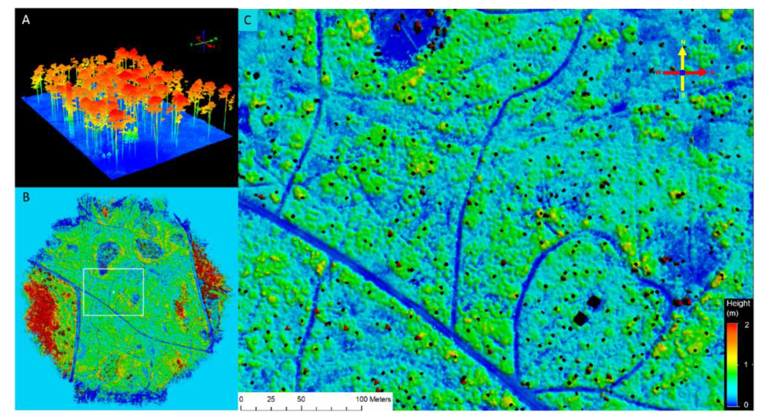
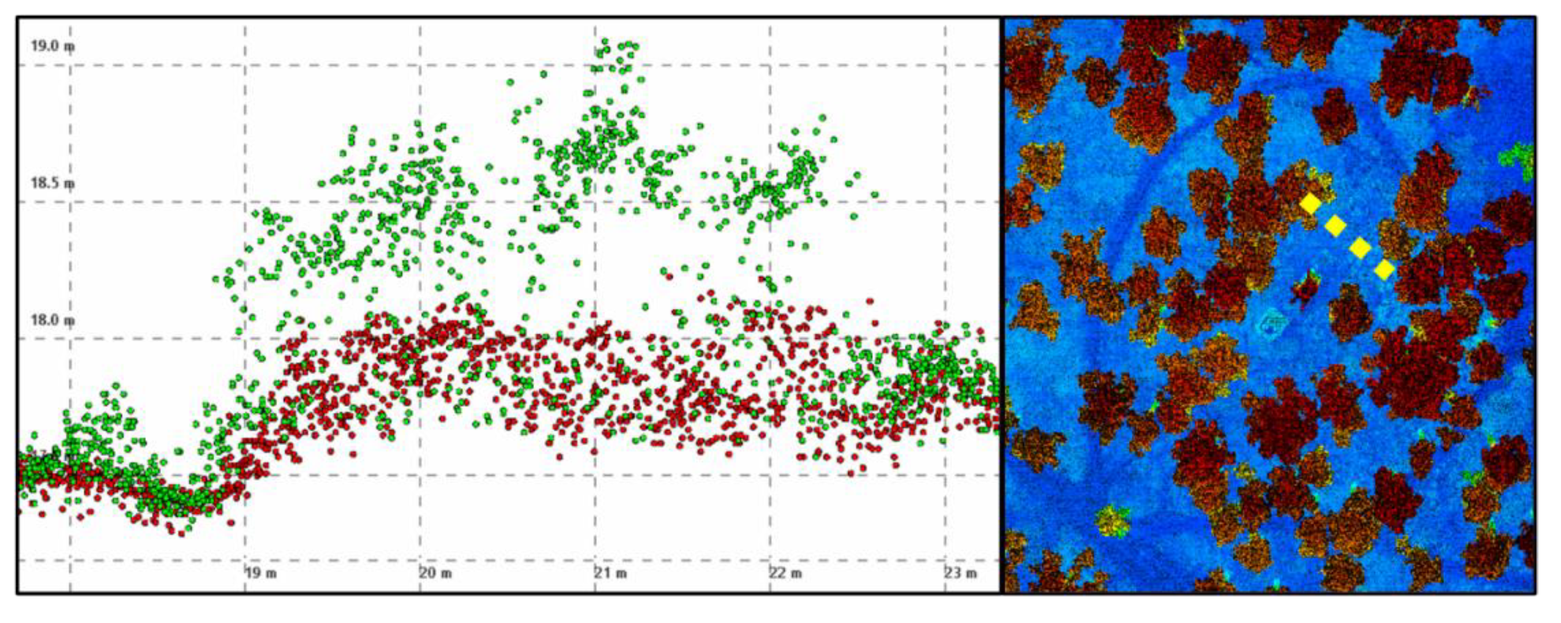
2.3. UAV-Borne LiDAR

We collected UAV-borne LiDAR using the GatorEye Unmanned Flying laboratory (www.gatoreye.org) on two separate dates corresponding to before (May 2018) and after (November 2018) the June 2018 fire, and were near-simultaneous to field-based understory height and biomass measurements. The GatorEye system included LiDAR, hyperspectral, thermal, and visual sensors, but in this study, we only used the LiDAR data. The LiDAR sensor was a Velodyne VLP-32c Ultra Puck dual-return sensor (Velodyne, San Jose, CA, USA), which had 32 separate lasers emitting 600,000 laser shots per second, resulting in a theoretical maximum of 1.2 million returns per second in dual return mode. This puck was integrated into a Phoenix Ultra Scout + (Phoenix LiDAR Systems, Austin, TX, USA), and the developer calculated the boresight parameters using Phoenix proprietary SpatialExplorer software. The GatorEye sensor suite was flown on a Matrice 600 Pro (DJI) hexacopter (SZ DJI Technology Co., Ltd., Shenzhen, China). Data collection parameters at the study site were: aboveground height (AGL) of 65–80 m, the ground speed of 10 m s⁻¹, and a side spacing of 40–50 m, resulting in an effective LiDAR sidelap of 70–90%. Data collection over the entire region required 4–8 flights per date, which were collected immediately following each other to reduce sources of noise in the final dataset (e.g., changes in satellite constellations or ionospheric conditions). The final area covered was a 250–300 m radius situated around the central eddy covariance tower, resulting in a total area of 28 ha (Figure 2). A detailed description of the system and data download is available at www.gatoreye.org.

During post-processing, we fused the differential base station (e.g., base) and GatorEye (e.g., rover) differential GNSS data with the Inertial Motion Unit (IMU: STIM 300, Sensoror, Horten, Norway) in Novatel Inertial Explorer software (version 8.7, Novatel Inc., Calgary, AB, Canada) and smoothed using Kalman Filters to produce the best estimate trajectories. We then merged the raw laser data with the trajectories using Phoenix SpatialExplorer (version 4.0.3, Austin, Texas, USA) software to produce standard LAS format LiDAR point cloud flightlines, which we then merged to produce a single point cloud with a point density of 800–1000 points m⁻². The points were distributed vertically, principally within the lower 5 m (understory) and between 20–30 m (tree crowns) above the ground level. To remove a small offset in point clouds between image collection dates, we shifted the May 2018 cloud to spatially match the November 2018 cloud, using the XYZ header offset in QT Modeller, and by calculating the average offset from 10 visible identifiers easily found in both clouds. The offset was less than 10 cm in XYZ.

We used the GatorEye Multi-Scale Post-Processing workflow (specifically version 207, which combines R scripts and packages with LAS Tools functions, and described in detail at www.gatoreye.org) to identify the ground return points from the raw point cloud, which were then interpolated to a raster GeoTIFF at 5 × 5 m resolution using a standard triangulation (TIN) approach to create the Digital Elevation Model (DEM). We then normalized the point cloud to this DEM and generated a high-resolution (0.25 × 0.25 m) raster digital surface model (DSM) of the top of the canopy. In the height normalized point cloud, we used the R packages LidR combined with the TreeLS treeMap function, using the map.hough approach, to automatically identify all tree stems directly and buffered these locations by 0.75 m to produce tree trunk maps across the study region.

To develop understory height maps, we subset the raw height points to only points between 0 and 6 m above the ground and erased any points occurring within the identified tree-trunk buffer regions. In this ‘understory height’ cloud (Figure 3), we reran the v207 GatorEye post-processing workflow, which provided digital surface model (DSM) products now for understory vegetation, over the DEM described above. We then created a raster version of the understory height at 0.5 × 0.5 m resolution to compare with field plot data, and specifically to calibrate and validate LiDAR-derived understory height and biomass maps.

We then clipped in Google Earth approximately 1 ha of the forested area surrounding each field plot; areas that underwent the same management and burn cycle as the central plot. The biomass maps were then stacked on the 1 ha areas for May and November 2018 data clipped from these four areas, and then the GeoTIFF raster data exported to spreadsheet format using IDL (ENVI v8.7) for further statistical analyses.

2.4. Statistical Analysis

We estimated the change in mean understory height and biomass before the fire, immediately after the fire, and five and twelve months after the fire for the field-plot measurements. A linear mixed-effect model with a nested ANOVA was used (the ‘lme’ package in RStudio) to examine how understory heights and biomass differed among different periods with plots nested within the wet and dry soil moisture groups. The TukeyHSD test was used to test for differences in height/biomass between different periods. Similarly, for LiDAR, we used the same model to contrast the changes in mean understory height before the fire and five months after the fire. A multiple regression model was used to assess the relationship between field height and biomass using soil moisture as a fixed variable. We compared the slopes (using ‘pairs’ function in ‘lsmeans’ package in RStudio) between May 2018 and November 2018 understory heights in order to determine whether there were any statistically significant differences between the relationship for the two time periods. For statistical evaluations, we calculated the correlation coefficient (r) to show the deviation between the two estimated height variables. We used absolute and relative root mean square errors (RMSE) (%) to explain the deviation of the predicted and measured heights.

To assess the difference in height vs. biomass for field and LiDAR measurements, we used a simple linear regression model to compare the relationships (Figure S1). Models (linear or quadratic) were investigated (May 2018, and November 2018, and combined heights) that best described the relationships between the understory field biomass and understory height estimated with LiDAR. For each model, regression assumptions were tested (using ‘autoplot’ function in ‘ggfortify’ package in RStudio). Slopes and intercepts comparisons were used to determine the significant difference between the two methods. We summarized the LiDAR-derived plot data using basic statistics for each plot and then used a paired t-test to compare before and after fire height and imputed biomass values across the plot. Finally, we used power analysis and the variance from LiDAR to estimate the required number of sample plots to detect the change in biomass after the fire.

3. Results

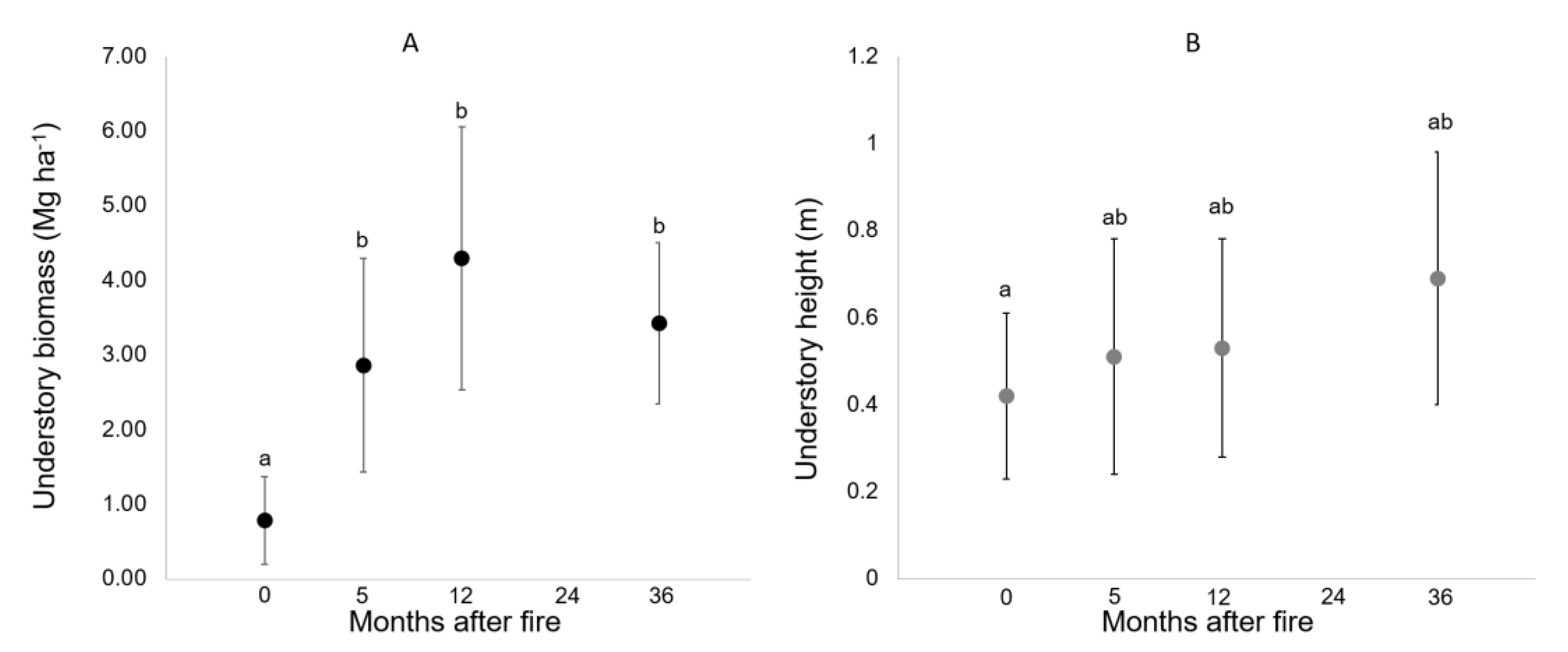
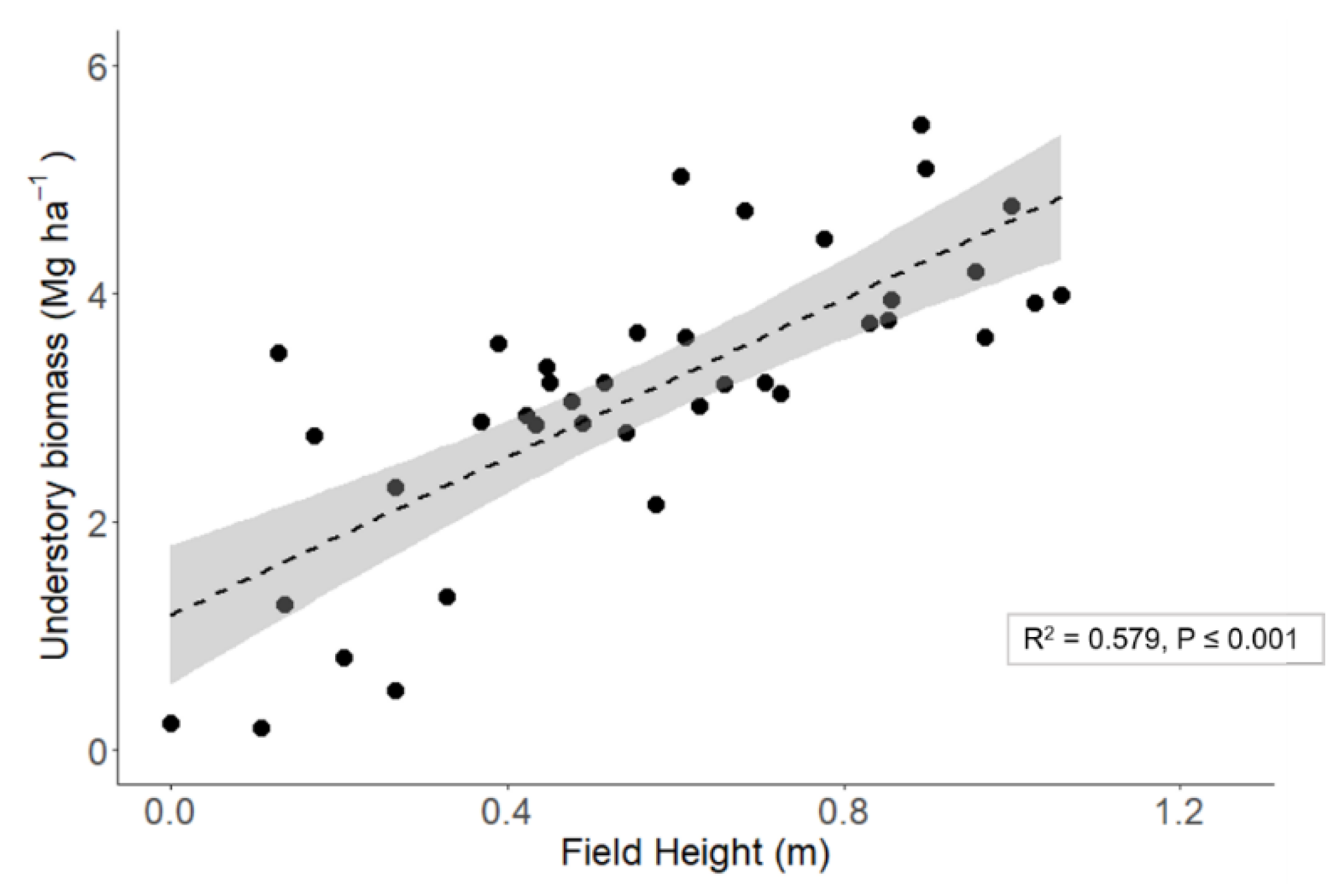
3.1. Field-Measured Aboveground Understory Biomass and Height

A month before the prescribed fire (May 2018) or 36 months since the previous fire, the field measurements estimated the average (± stdev) aboveground understory biomass to be 3.42 ± 1.08 Mg ha⁻¹ (Figure 4A). The prescribed fire occurred in June 2018, and the understory biomass was remeasured ~one week (0 months) following the fire, which indicated that only ~23% of living understory biomass remained (0.79 ± 0.59 Mg ha⁻¹) (Figure 4A). While overall average understory biomass decreased immediately after the fire, almost 84% of the biomass was recovered within five months (2.86 ± 1.43 Mg ha⁻¹ in November 2018), and after 12 months, the understory biomass had returned to near pre-fire conditions (4.29 ± 1.76 Mg ha⁻¹ in June 2019) (Figure 4A). The t-test used to compare the mean difference between 36 months (pre-fire) and 0 months (post-fire) showed a significant difference in biomass (p ≤ 0.001) (Figure 4A). However, there was no significant difference among 36 (pre-fire) vs. five months after the fire: (p = 0.177) or the 36 vs. 12 months after the fire (p = 0.070). The nested ANOVA showed that fire had a significant effect on biomass (F-value = 27.79, p ≤ 0.001) as the biomass dropped immediately after the fire (0 months), however, biomass change for 5, 12, and 36 months after the fire did not differ from one another.

Using field measurements, the average (±stdev) understory height pre-fire (May 2018) was found to be 0.68 ± 0.29 m. After the prescribed fire in June 2018, the average height of the remaining live understory vegetation was reduced to 0.42 ± 0.19 m. The average height of the understory recovered within five months of fire (0.51 ± 0.27 m) and gained little height 12 months post-fire (0.53 ± 0.25 m). The nested ANOVA used to assess the variation between the groups showed that fire had a significant effect on height (F-value = 2.96, p = 0.038). The t-test showed significant difference in height between 36 months (pre-fire) and 0 months (post-fire) (p = 0.002) (Figure 4B). However, there was no significant difference among two time periods 36 (pre-fire) vs. 5 months after the fire: (p = 0.065) or the 36 vs. 12 months after the fire (p = 0.094).

The multiple regression model between height and biomass did not indicate soil moisture was significant (p = 0.295) for either the 36 months or five-month harvest. The comparison among time periods for the relationship between field height and field biomass indicated they were not different, and the combined equation showed a significant positive relationship between the two variables (R² = 0.579, p ≤ 0.001, N = 20) (Equation (3); Figure 5).

$$Understory biomass =1.182 + 3.461\times Field height$$

(3)

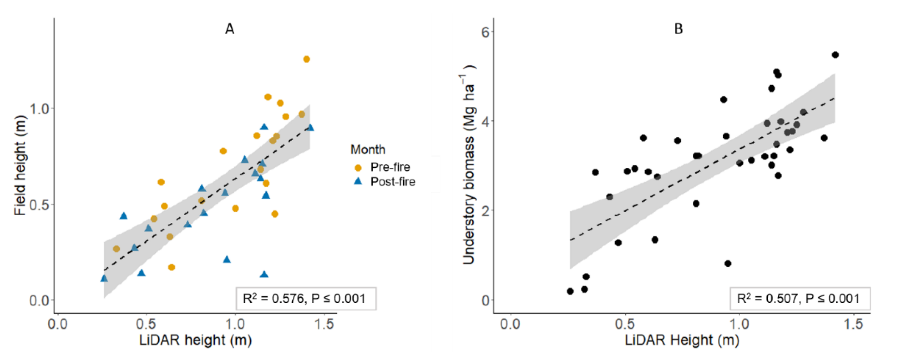
3.2. LiDAR Relationship with Field-Measured Understory Height and Biomass

Before the fire, LiDAR estimated the average (± stdev) understory vegetation height to be 0.98 ± 0.32 m. The average height of the understory changed to 0.84 ± 0.35 m five months after the fire. The t-test did not show any significant difference in mean understory height between the two time periods (p = 0.201).

Mean understory height estimates calculated from LiDAR had a significant positive correlation with field-based mean height measurements for both pre-fire (May 2018, R² = 0.617, p ≤ 0.001, n = 20) and 5 months post-fire (November 2018, R² = 0.495, p ≤ 0.001, n = 20) (Figure 6A). No significant differences were found in slope (p = 0.766) or intercept (p = 0.911) between the two time periods (slope: May 2018 = 0.877, November 2018 = 0.957). Thus, we combined the two datasets from two different months for an examination of the LiDAR height vs. biomass relationship. The values obtained from LiDAR had an average understory height of 0.91 ± 0.34 m. The field measured understory height had an average of 0.58 ± 0.30 m. The combined LiDAR height estimates regressed against the corresponding field height measurements showed a significant positive relationship with R² = 0.576 (p ≤ 0.001, n = 40) (Figure 6A), a correlation coefficient (r) of 0.770, and an absolute RMSE of 0.216 m (relative RMSE of 18.61%).

LiDAR-derived understory heights (May 2018 and November 2018) were directly compared with field measured dry understory biomass, collected at the same field plots used for height measurements (Figure 6B). The goodness-of-fit analysis showed the best model form was a linear regression, with biomass versus combined height providing the highest R² value (R² = 0.507, p ≤ 0.001, n = 40). Similar to the equation for field height, the intercept was above zero but was closer to zero than for field measurements (Equations (3) and (4)).

$$Understory biomass =0.616 + 2.750\times LiDAR height$$

(4)

Slope and intercept comparisons performed to compare understory biomass with the field- and LiDAR- derived understory height estimates (Equations (3) and (4)) showed no significant difference between the two methods (slope: field = 3.461, LiDAR = 2.750, p = 0.278, and intercept: p = 0.272).

3.3. LiDAR Biomass and Change at the Plot Scale

The areas of plots 1–4 were 0.11, 0.10, 0.15, and 0.16 ha, as was defined by the positions of trees monitored for growth and after removing the wetland areas. However, this area included the tree and trunk buffer regions (0.75 m), which were removed for understory analysis (described in Methods). In May 2018 (pre-fire), the mean plot biomass estimated with LiDAR ranged from 2.87 to 3.34 Mg ha⁻¹, while in November 2018 (five months post-fire), the mean plot biomass changed to 2.40 to 2.75 Mg ha⁻¹, or a 12.7% reduction (

Table 1. Number of 0.5 × 0.5 m pixels (N), and the biomass (Mg ha⁻¹) minimum (Min), maximum (Max), Mean, standard deviation (Stdev), and change for each plot and flight. The before fire UAV LiDAR flight occurred on the 3/5/2018, and after the fire, it occurred on the 3/11/2018. Here, the dashed line (-) indicates that the change was not estimated.

LiDAR Flight	Plot	N	Min	Max	Mean	Stdev
Before fire	1	4635	1.00	6.31	3.01	0.87
	2	3441	0.86	17.13	3.13	0.92
	3	6185	1.03	17.13	2.87	0.97
	4	6262	0.94	17.15	3.34	1.39
After fire	1	4633	0.94	7.93	2.40	0.74
	2	3441	0.83	17.01	2.74	0.92
	3	6186	0.92	17.15	2.63	0.94
	4	6329	0.80	17.15	2.75	1.29
Change (after-before)	1	-	-	-	−0.61	-
	2	-	-	-	−0.39	-
	3	-	-	-	−0.24	-
	4	-	-	-	−0.59	-

). The field sampling method estimated a ~16% reduction in biomass five months post-fire and was much more variable than the estimates from LiDAR (Figure 7). The power analysis using estimated biomass from LiDAR indicated that the field sampling method would have required 59 1 × 1 m sample subplots to detect the estimated 12.7% reduction in biomass.

4. Discussion

For this flatwoods pine savanna, understory vegetation biomass was reduced by ~77% immediately after the fire (Figure 4A). However, the biomass quickly recovered within only a few months, and after one year, the fire’s effect on the understory structure was nearly indiscernible. Similar studies [38,39,40] have also shown the notable resilience of the understory to fire in southern pine ecosystems. The rapid return of understory height and biomass highlights the potential for fuel loads to build and for the soil surface environment to change very quickly post-fire in these ecosystems. Given the fairly consistent temporal dynamic of understory recovery across multiple studies at this site (Figure 4A) [38,39,40], focus could be better placed on the spatial distribution of understory recovery as it is clearly an important feature in determining where pine regeneration could occur and where key understory species (e.g., Aristida stricta) might be found within flatwood pine ecosystems.

The LiDAR approach captured the spatial distribution of understory height and biomass (e.g., Figure 2 and Figure 3) likely as well or better than field-based estimates. Interestingly, both methods returned estimates of positive biomass at the X-intercept for the heights vs. biomass equations (Figure 5 and Figure 6B), with the field sampling estimating a greater intercept. Because LiDAR measured more points within a subplot than the field sampling, it may have better-captured biomass variation than the field measurements. Moreover, relationships between field height and understory biomass likely have an upper limit in accuracy, similar to what is observed in the allometric relationship between individual plant height and biomass [37]. Where the upper limit for biomass prediction might exist with UAV technology remains unclear, as additional sensors (e.g., hyperspectral, thermal) on the UAV, advances in LiDAR technology, or UAV flight protocols (e.g., speed, height) could likely further improve prediction accuracy in characterizing understory height and biomass with this technology [27]. In addition, DEM accuracy could be improved with additional flights or accounting for changes in ground surface with forest development [41], as fire changes the actual ground surface by consuming the forest floor. Although these factors would further complicate the accuracy of LiDAR data to estimate understory parameters, the potential for further improvements in the application of UAV technology and the resulting spatial information suggests that remote sensing approaches should be explored to manage the understory of these ecosystems.

The high-density LiDAR point cloud data in this study showed that high-resolution LiDAR, with adequate canopy penetration, can be quite effective in quantifying understory height (R² = 0.58) and biomass (R² = 0.51). These findings are similar to the previous study by Su and Bork [23], where they used LiDAR data (0.54 points m⁻²) to estimate understory height (R² = 0.23) in an open Populus forest. Similarly, Jakubowksi et al. [25] successfully estimated the height of understory biomass using the combination of high-density airborne LiDAR (~9 points m⁻²) and multispectral imagery (R² = 0.59). In this study, we focused on using only LiDAR to estimate understory height and biomass, but further improvements in predicting biomass might be possible with additional sensors (e.g., hyperspectral).

The variance in LiDAR estimates of heights and biomass suggested that the change caused by fire could have only been captured if ~0.6% of the studied area had been sampled for biomass. Our 20 clipped plots, or 0.2% of the overall plot area, resulted in highly variable estimates of biomass change after the fire, with one plot even recording increased biomass (Figure 7). Accurate destructive sampling would mean increasing the number of clipped plots in this study from 20 to 59, with an equivalent increase in the field and lab time from ~40 to ~120 h. Thus, the slight reduction in explained variance using height to estimated biomass with LiDAR versus with field measurements is likely to have less of an impact on achieving management objectives than the benefits associated with savings in time and expense. In addition, mapping the spatial arrangement of understory heights and other features (e.g., wetlands, fire breaks, buildings) (Figure 2) would facilitate fire management, potentially saving time, reducing the threat of escaped fire, and an optimal approach to achieving the management objectives for a savanna system. An additional time-savings is indicated by the consistency in the LiDAR height vs. biomass equations across time, which suggests a robust calibrated equation could be created with a limited number of harvests.

5. Conclusions

We found that understory structure, specifically height and biomass, recovered quickly after the fire in these flatwood pine savannas. In general, this is consistent with past studies that used clipped plots, but here we find that the LiDAR measurements provide reasonable estimates of understory height and thus can be used to describe understory biomass in a more spatially explicit manner than what is feasible with a field sampling approach. The understory vegetation map produced in this study could be used by forest managers or ecologists to aid in a prescribed fire application by predicting fire behavior. In addition to benefitting restoration efforts, this approach to remote sensing could help scientists understand the controls on the spatial variability in ecosystem processes. Future research is recommended that explores the intersection between the spatial distribution of understory heights and ecological function.

References

1. Frost, C.C. Four centuries of changing landscape patterns in the longleaf pine ecosystem. In Proceedings of the Tall Timbers Fire Ecology Conference, Tallahassee, FL, USA, 3–6 November 1993; pp. 17–43. [Google Scholar]
2. Landers, J.L.; Van Lear, D.H.; Boyer, W.D. The longleaf pine forests of the southeast: Requiem or renaissance? J. For. 1995, 93, 39–44. [Google Scholar]
3. Abrams, M.D. Fire and the development of oak forests. BioScience 1992, 42, 346–353. [Google Scholar] [CrossRef]
4. Earley, L.S. Looking for Longleaf: The Fall and Rise of an American Forest; Univ of North Carolina Press: Chapel Hill, NC, USA, 2004. [Google Scholar]
5. Mitchell, R.J.; Hiers, J.K.; O’Brien, J.J.; Jack, S.; Engstrom, R. Silviculture that sustains: The nexus between silviculture, frequent prescribed fire, and conservation of biodiversity in longleaf pine forests of the southeastern united states. Can. J. For. Res. 2006, 36, 2724–2736. [Google Scholar] [CrossRef] [Green Version]
6. Frost, C. History and future of the longleaf pine ecosystem. In The Longleaf Pine Ecosystem; Springer: New York, NY, USA, 2007; pp. 9–48. [Google Scholar]
7. McEwan, R.W.; Dyer, J.M.; Pederson, N. Multiple interacting ecosystem drivers: Toward an encompassing hypothesis of oak forest dynamics across eastern north america. Ecography 2011, 34, 244–256. [Google Scholar] [CrossRef]
8. Kirkman, L.K.; Mitchell, R.J. Conservation management of pinus palustris ecosystems from a landscape perspective. Appl. Veg. Sci. 2006, 9, 67–74. [Google Scholar] [CrossRef]
9. Pecot, S.D.; Mitchell, R.J.; Palik, B.J.; Moser, E.B.; Hiers, J.K. Competitive responses of seedlings and understory plants in longleaf pine woodlands: Separating canopy influences above and below ground. Can. J. For. Res. 2007, 37, 634–648. [Google Scholar] [CrossRef]
10. Nowell, H.; Holmes, C.; Robertson, K.; Teske, C.; Hiers, J. A new picture of fire extent, variability, and drought interaction in prescribed fire landscapes: Insights from florida government records. Geophys. Res. Lett. 2018, 45, 7874–7884. [Google Scholar] [CrossRef] [Green Version]
11. Sharma, A.; Brethauer, D.K.; McKeithen, J.; Bohn, K.K.; Vogel, J.G. Prescribed burn effects on natural regeneration in pine flatwoods: Implications for uneven-aged stand conversion from a florida study. Forests 2020, 11, 328. [Google Scholar] [CrossRef] [Green Version]
12. Robertson, K.M.; Platt, W.J.; Faires, C.E. Patchy fires promote regeneration of longleaf pine (pinus palustris mill.) in pine savannas. Forests 2019, 10, 367. [Google Scholar] [CrossRef] [Green Version]
13. Riano, D.; Meier, E.; Allgöwer, B.; Chuvieco, E.; Ustin, S.L. Modeling airborne laser scanning data for the spatial generation of critical forest parameters in fire behavior modeling. Remote Sens. Environ. 2003, 86, 177–186. [Google Scholar] [CrossRef]
14. García, M.; Riaño, D.; Chuvieco, E.; Salas, J.; Danson, F.M. Multispectral and lidar data fusion for fuel type mapping using support vector machine and decision rules. Remote Sens. Environ. 2011, 115, 1369–1379. [Google Scholar] [CrossRef]
15. Wulder, M.; White, J.; Alvarez, F.; Han, T.; Rogan, J.; Hawkes, B. Characterizing boreal forest wildfire with multi-temporal landsat and lidar data. Remote Sens. Environ. 2009, 113, 1540–1555. [Google Scholar] [CrossRef]
16. Bishop, B.D.; Dietterick, B.C.; White, R.A.; Mastin, T.B. Classification of plot-level fire-caused tree mortality in a redwood forest using digital orthophotography and lidar. Remote Sens. 2014, 6, 1954–1972. [Google Scholar] [CrossRef] [Green Version]
17. Sato, L.Y.; Gomes, V.C.F.; Shimabukuro, Y.E.; Keller, M.; Arai, E.; Dos-Santos, M.N.; Brown, I.F. Post-fire changes in forest biomass retrieved by airborne lidar in amazonia. Remote Sens. 2016, 8, 839. [Google Scholar] [CrossRef] [Green Version]
18. McCarley, T.R.; Kolden, C.A.; Vaillant, N.M.; Hudak, A.T.; Smith, A.M.; Wing, B.M.; Kellogg, B.S.; Kreitler, J. Multi-temporal lidar and landsat quantification of fire-induced changes to forest structure. Remote Sens. Environ. 2017, 191, 419–432. [Google Scholar] [CrossRef] [Green Version]
19. Kwak, D.-A.; Chung, J.; Lee, W.-K.; Kafatos, M.; Lee, S.Y.; Cho, H.-K.; Lee, S.-H. Evaluation for damaged degree of vegetation by forest fire using lidar and a digital aerial photograph. Photogramm. Eng. Remote Sens. 2010, 76, 277–287. [Google Scholar] [CrossRef]
20. Kane, V.R.; Lutz, J.A.; Roberts, S.L.; Smith, D.F.; McGaughey, R.J.; Povak, N.A.; Brooks, M.L. Landscape-scale effects of fire severity on mixed-conifer and red fir forest structure in yosemite national park. For. Ecol. Manag. 2013, 287, 17–31. [Google Scholar] [CrossRef]
21. Clark, K.L.; Skowronski, N.; Hom, J.; Duveneck, M.; Pan, Y.; Van Tuyl, S.; Cole, J.; Patterson, M.; Maurer, S. Decision support tools to improve the effectiveness of hazardous fuel reduction treatments in the new jersey pine barrens. Int. J. Wildland Fire 2009, 18, 268–277. [Google Scholar] [CrossRef]
22. Skowronski, N.S.; Clark, K.L.; Duveneck, M.; Hom, J. Three-dimensional canopy fuel loading predicted using upward and downward sensing lidar systems. Remote Sens. Environ. 2011, 115, 703–714. [Google Scholar] [CrossRef]
23. Su, J.G.; Bork, E.W. Characterization of diverse plant communities in aspen parkland rangeland using lidar data. Appl. Veg. Sci. 2007, 10, 407–416. [Google Scholar] [CrossRef]
24. Estornell, J.; Ruiz, L.; Velázquez-Martí, B.; Fernández-Sarría, A. Estimation of shrub biomass by airborne lidar data in small forest stands. For. Ecol. Manag. 2011, 262, 1697–1703. [Google Scholar] [CrossRef] [Green Version]
25. Jakubowksi, M.K.; Guo, Q.; Collins, B.; Stephens, S.; Kelly, M. Predicting surface fuel models and fuel metrics using lidar and cir imagery in a dense, mountainous forest. Photogramm. Eng. Remote Sens. 2013, 79, 37–49. [Google Scholar] [CrossRef] [Green Version]
26. Greaves, H.E.; Vierling, L.A.; Eitel, J.U.; Boelman, N.T.; Magney, T.S.; Prager, C.M.; Griffin, K.L. High-resolution mapping of aboveground shrub biomass in arctic tundra using airborne lidar and imagery. Remote Sens. Environ. 2016, 184, 361–373. [Google Scholar] [CrossRef]
27. Beland, M.; Parker, G.; Sparrow, B.; Harding, D.; Chasmer, L.; Phinn, S.; Antonarakis, A.; Strahler, A. On promoting the use of lidar systems in forest ecosystem research. For. Ecol. Manag. 2019, 450, 117484. [Google Scholar] [CrossRef]
28. De Almeida, D.R.A.; Almeyda Zambrano, A.M.; Broadbent, E.N.; Wendt, A.L.; Foster, P.; Wilkinson, B.E.; Salk, C.; Papa, D.d.A.; Stark, S.C.; Valbuena, R. Detecting successional changes in tropical forest structure using gatoreye drone-borne lidar. Biotropica 2020, 52, 1155–1167. [Google Scholar] [CrossRef]
29. Dalla Corte, A.P.; Souza, D.V.; Rex, F.E.; Sanquetta, C.R.; Mohan, M.; Silva, C.A.; Zambrano, A.M.A.; Prata, G.; de Almeida, D.R.A.; Trautenmüller, J.W. Forest inventory with high-density uav-lidar: Machine learning approaches for predicting individual tree attributes. Comput. Electron. Agric. 2020, 179, 105815. [Google Scholar] [CrossRef]
30. Thiel, C.; Schmullius, C. Comparison of uav photograph-based and airborne lidar-based point clouds over forest from a forestry application perspective. Int. J. Remote Sens. 2017, 38, 2411–2426. [Google Scholar] [CrossRef]
31. D’Oliveira, M.V.; Broadbent, E.N.; Oliveira, L.C.; Almeida, D.R.; Papa, D.A.; Ferreira, M.E.; Zambrano, A.M.A.; Silva, C.A.; Avino, F.S.; Prata, G.A. Aboveground biomass estimation in amazonian tropical forests: A comparison of aircraft-and gatoreye uav-borne lidar data in the chico mendes extractive reserve in acre, brazil. Remote Sens. 2020, 12, 1754. [Google Scholar] [CrossRef]
32. Peet, R.K.; Allard, D.J. Longleaf Pine Vegetation of the Southern Atlantic and Eastern Gulf Coast Regions: A Preliminary Classification. In Proceedings of the Tall Timbers Fire Ecology Conference, Tallahassee, FL, USA, 3–6 November 1993; pp. 45–81. [Google Scholar]
33. Powell, T.L.; Starr, G.; Clark, K.L.; Martin, T.A.; Gholz, H.L. Ecosystem and understory water and energy exchange for a mature, naturally regenerated pine flatwoods forest in north florida. Can. J. For. Res. 2005, 35, 1568–1580. [Google Scholar] [CrossRef]
34. Powell, T.L.; Gholz, H.L.; Clark, K.L.; Starr, G.; Cropper Jr, W.P.; Martin, T.A. Carbon exchange of a mature, naturally regenerated pine forest in north florida. Glob. Chang. Biol. 2008, 14, 2523–2538. [Google Scholar] [CrossRef]
35. National Centers for Environmental Information: National Oceanic and Atmospheric Administration. Available online: https://www.Ncdc.Noaa.Gov./cdo-web/datatools/findstation (accessed on 5 August 2020).
36. Heady, H.F. The measurement and value of plant height in the study of herbaceous vegetation. Ecology 1957, 38, 313–320. [Google Scholar] [CrossRef] [Green Version]
37. Gholz, H.; Guerin, D.; Cropper, W. Phenology and productivity of saw palmetto (serenoa repens) in a north florida slash pine plantation. Can. J. For. Res. 1999, 29, 1248–1253. [Google Scholar] [CrossRef]
38. Kirkman, L.K.; Mitchell, R.J.; Helton, R.C.; Drew, M.B. Productivity and species richness across an environmental gradient in a fire-dependent ecosystem. Am. J. Bot. 2001, 88, 2119–2128. [Google Scholar] [CrossRef] [PubMed]
39. Abrahamson, W.G.; Abrahamson, C.R. Post-fire canopy recovery in two fire-adapted palms, serenoa repens and sabal etonia (arecaceae). Fla. Sci. 2006, 69, 69–79. [Google Scholar]
40. Lavoie, M.; Starr, G.; Mack, M.; Martin, T.; Gholz, H. Effects of a prescribed fire on understory vegetation, carbon pools, and soil nutrients in a longleaf pine-slash pine forest in florida. Nat. Areas J. 2010, 30, 82–94. [Google Scholar] [CrossRef]
41. Fisher, P.F.; Tate, N.J. Causes and consequences of error in digital elevation models. Prog. Phys. Geogr. 2006, 30, 467–489. [Google Scholar] [CrossRef]
Figure 1. Images depicting (A) map of the state of Florida, USA extracted from world imagery basemap in ArcGIS; (B) location of Austin Cary Forest within Florida, and (C) the four 50 × 50 m permanent plots (white squares) that were used to monitor overstory dynamics and where the five understory samplings per plot were placed (locations not shown).
Forests 12 00038 g001
Figure 2. LiDAR images depicting (A) a select part of the study area that shows the ground surface, understory, and trees, (B) an understory canopy height map (CHM) estimated for the fire management unit and a ~6.5-hectare area (white rectangle) around the eddy-covariance tower, and (C) an understory CHM for the selected area showing the removed eddy-covariance tower, support structure (black squares), and trees (black dots). Near continuous blue areas are wetland depressions, roads, or fire breaks. Blue is the lowest understory canopy height (0 m or ground surface), and red is the highest (2 m).
Forests 12 00038 g002
Figure 3. Pre- (Green) and Post-fire (Red) LiDAR point clouds for a 6 m sample profile along the transect presented in (Right) the overview map as a yellow dash line (Left).
Forests 12 00038 g003
Figure 4. Mean ± stdev understory biomass (A) and height (B) at different months after a prescribed fire (June 2018) using the field harvest method. Here, 0, 5, and 12 represented the months when the measurements were collected after the fire and 36 the months since a 2015 fire but immediately before the 2018 fire (pre-fire). Note: LiDAR data was collected pre-fire- and five months post-fire.
Forests 12 00038 g004
Figure 5. Relationship between field height (m) and understory biomass (Mg ha−1) along with the confidence interval of the regression line.
Forests 12 00038 g005
Figure 6. (A) Comparison between field understory height (m) and LiDAR understory height (m) for two sample dates that fell before (May 2018) and five months after (November 2018) a prescribed fire. (B) Relationship between LiDAR height (m) and understory biomass (Mg ha−1) along with the confidence interval of the regression lines.
Forests 12 00038 g006
Figure 7. Pixel-scale (0.5 × 0.5 m) LiDAR-derived biomass compared to biomass-derived from field sampling method before (Pre-) and after (Post-) the 2018 prescribed fire for each plot area.
Forests 12 00038 g007