Article

Simulation of Vegetation Cover Based on the Theory of Ecohydrological Optimality in the Yongding River Watershed, China

1
School of Soil and Water Conservation, Beijing Forestry University, Beijing 100083, China
2
Key Laboratory of State Forestry Administration on Soil and Water Conservation, Beijing 100083, China
3
Inner Mongolia Ulanqab Meteorological Bureau, Ulanqab 012000, China
*
Author to whom correspondence should be addressed.
Forests 2021, 12(10), 1377; https://doi.org/10.3390/f12101377
Submission received: 11 August 2021 / Revised: 6 October 2021 / Accepted: 8 October 2021 / Published: 10 October 2021
(This article belongs to the Section Forest Hydrology)

Abstract

:
During ecological restoration, it is necessary to comprehensively consider the state of vegetation in climate–soil–vegetation systems. The theory of ecohydrological optimality assumes that this state tends to reach long-term dynamic equilibrium between the available water supply of the system and the water demand of vegetation, which is driven by the maximization of productivity. This study aimed to understand the factors that affect the spatial distribution of vegetation and simulate the ideal vegetation coverage (M0) that a specific climate and soil can maintain under an equilibrium state. The ecohydrological optimality model was applied based on meteorological, soil, and vegetation data during the 2000–2018 growing seasons, and the sensitivity of the simulated results to input data under distinct vegetation and soil conditions was also considered in the Yongding River watershed, China. The results revealed that the average observed vegetation coverage (M) was affected by precipitation characteristic factors, followed by wind speed and relative humidity. The M, as a whole, exhibited horizontal zonal changes from a spatial perspective, with an average value of 0.502, whereas the average M0 was 0.475. The ecohydrological optimality theory ignores the drought resistance measures evolved by vegetation in high vegetation coverage areas and is applicable to simulate the long-term average vegetation coverage that minimizes water stress and maximizes productivity. The differences between M and M0 increased from the northwest to the southeast of this area, with a maximum value exceeding 0.3. Meteorological factors were the most sensitive factors of this model, and the M0 of the steppe was most sensitive to the stem fraction, mean storm depth, and air temperature. Whether soil factors are sensitive depends on soil texture. Overall, the study of the carrying capacity of vegetation in the natural environment contributes to providing new insights into vegetation restoration and the conservation of water resources.

1. Introduction

Vegetation, as the primary component of terrestrial ecosystems, interacts with hydrological processes [1,2]. The spatiotemporal responses of vegetation to water circulation mainly depend on the climate, soil, and physiological characteristics of the vegetation [3,4,5]. Precipitation is linked to vegetation through soil moisture [6]. The uncertainty of both the frequency and amount of precipitation promotes vegetation to optimize productivity [7,8]. Moreover, the soil texture is responsible for the differences in the hydraulic properties of the root zone soil and further impacts the spatial distribution of soil moisture [9]. The water available for use by vegetation in the soil increases from coarse sand, fine sand, sandy soil, loam to clay [10]. Clayey soils generally support shallow-rooted vegetation, and sandy soils favor deep-rooted vegetation [11]. Likewise, the physiological responses of plant species to moisture changes are related to their own structure and strategies for adaptation to drought, such as the crown shape, xylem structures, size and depth of roots, and leaf traits [12,13,14,15]. Diverse vegetation types show differences in water utilization efficiency and stomatal regulation, which are reflected by canopy conductance [16]. For instance, when vegetation is under water stress, reductions in the vegetation height, branch leaf area-to-sapwood area ratio, and leaf size could improve hydraulic efficiency and limit xylem tension [17,18]. The prevalent view is that natural selection and adaptation capability lead to the evolution of vegetation to the optimal state in climate–soil–vegetation systems for long periods of time [19]. Different studies have emphasized this optimal state differently, such as the stomatal optimization model from the perspective of plant physiology or the feasibility of vegetation patterns from the perspective of semiarid watersheds [20,21]. Fewer studies have considered the underlying mechanism of the optimal state from the combined aspects of vegetation physiology and hydrological processes.
This study used the theory of ecohydrological optimality proposed by Eagleson [22] (p. 341), which states that vegetation tends to prefer an average state of zero plant stress under given climate and soil conditions driven by productivity maximization [23]. Based on the precondition that the precipitation process obeys the Poisson distribution, a mathematical and physical expression of the water balance equation was established [24,25,26,27,28,29,30,31,32]. Then, the response of stomata to the available water of vegetation and light is idealized and the potential canopy conductance equation and water balance equation are coupled to formulate this average state of vegetation [23]. This model was improved, and its parameters as well as applicable conditions were subsequently verified by many scholars [33,34,35,36,37,38]. Furthermore, the advancement of satellite measurements as well as the feasibility and universality of ground surveys in China also provide plenty of data for model research [39]. For example, Mo [40] and Cong [41] compared the actual vegetation cover generated by the remotely sensed normalized difference vegetation index (NDVI) with the simulated cover from the model output and verified the applicability of the model in the Horqin Sands in China and the Northeast China Transect. Overall, the ecohydrological optimality model can obtain the ideal vegetation coverage ( M 0 ) to maximize productivity and minimize water stress in water-limited or energy-limited ecosystems.
The Yongding River watershed is an important water source conservation area and ecological corridor in the Beijing–Tianjin–Hebei region of China. The upper reaches of the basin are mountainous areas with steep slopes and an uneven distribution of vegetation, and these areas are prone to soil erosion. The lower reaches are plain areas, where the ecosystem is degraded and the river is cut off. China has formulated a series of comprehensive control and ecological restoration measures. The aim of these measures is to restore the local ecosystem to a sustainable natural state. Vegetation cover can represent the growth status of vegetation to a certain extent, and it can be used as a reference index for ecological restoration. Zhang [42] discussed the problem of excessive vegetation restoration in the “Grain-to-Green Program”, which was implemented over the Loess Plateau of China, and considered that the M 0 value of the model can be used as a limit for afforestation. Hence, research on the ecohydrological optimality model has practical significance for artificially improving the quality and stability of ecosystems.
Although the statistical–dynamical water balance model of Eagleson is well recognized, the theory of ecohydrological optimality is still controversial and needs to be verified in dissimilar regions and vegetation types [43]. In addition, vegetation types were rarely classified in detail and were not comprehensively considered together with soil texture and precipitation characteristics in previous related studies. In this context, the primary objectives of this study were to (1) analyze the spatial distribution characteristics and impact factors of the observed vegetation coverage ( M ) during the growing season from 2000 to 2018; (2) evaluate the applicability of ecohydrological optimality theory in the Yongding River watershed; (3) calculate the simulated M 0 value based on local meteorological, soil, and vegetation factors; and (4) investigate the sensitivity of the model to input parameters under varied vegetation and soil conditions. The results of this study provide detailed theoretical guidance and a scientific assessment of the application of ecological restoration and water resource management.

2. Materials and Methods

2.1. Study Area

The Yongding River watershed (Figure 1a), crossing five provinces (Inner Mongolia, Shanxi, Hebei, Beijing, and Tianjin), is located southwest of Beijing (112°–117°45′ E and 38°27′–41°20′ N). The total area of this watershed is 47,016 km2, with high elevations in the northwest and low elevations in the southeast, including mountain areas (45,063 km2) and plain areas (1953 km2), with Sanjiadian as the boundary. The average groundwater depth in the plain area is 4–50 m, most of which is more than 20 m (data were developed by the website of Ministry of Water Resources of the People’s Republic of China http://www.mwr.gov.cn/ accessed on 29 January 2019). The area has a temperate continental monsoon climate, with mean annual precipitation from 360 mm to 650 mm, a mean annual temperature of 6.9 °C, and a mean annual runoff of 12.13 mm (averaged from 1963 to 2018). The vegetation growing season in this region is from April to September since the precipitation is concentrated and the temperature is optimum during this period. Major vegetation types include needleleaf forest, broadleaf forest, scrub, steppe, and cultural vegetation, where cultural vegetation refers to the phytocommunity formed by artificial cultivation, including irrigated or nonirrigated crops and deciduous orchards (Figure 1b). The main soil texture types are clay loam and sandy loam (Figure 1c).

2.2. Data Preparation

Digital elevation model (DEM) data were used to divide the watershed boundaries, with a resolution of 30 m, provided by the Geospatial Data Cloud site, Computer Network Information Center, Chinese Academy of Sciences (http://www.gscloud.cn accessed on 1 December 2009). Then the spatial distributions of vegetation types and soil texture types were obtained from the Data Center for Resources and Environmental Sciences, Chinese Academy of Sciences (RESDC) (http://www.resdc.cn accessed on 30 May 2001) with a resolution of 1 km. We obtained NDVI from the MOD13A3 (monthly 1-km) VI product from 2000 to 2018 to analyze the spatial distribution of M . The method of converting NDVI data into M was improved by Li [44]:
M = NDVI NDVI min NDVI max NDVI min
We assumed that the maximum coverage of forest and the minimum coverage of barren land in the study area were 100% and 0%, respectively, corresponding to the maximum and minimum values of NDVI. Due to inevitable image noise, NDVI max and NDVI min are the maximum and minimum NDVI values, respectively, in the 95% confidence interval, spanning 19 years. The effective value range of the MOD13A3 product is from −0.2 to 1, while water bodies have NDVI values less than 0. NDVI max and NDVI min are 0.71 and 0.16, respectively, in this study.
The input data and parameters (which are listed and explained in Table 1 and Table 2) required to run the model include vegetation data, meteorological data, and soil data, among which the empirical parameters are derived from previous studies and the leaf area index (LAI) was obtained from the MCD15A2H (8-day 500-m) product. Multiple meteorological datasets were required to calculate the precipitation characteristic factors ( m h , m υ , m t r , and m t b ) and the potential evaporation using the Penman–Monteith equation [45]. Daily precipitation, average air temperature, maximum air temperature, minimum air temperature, sunshine duration, wind speed, and relative humidity data from 2000 to 2018 were acquired from 66 meteorological stations (Figure 1a) across the study area by the China Meteorological Data Service Center (http://data.cma.cn accessed on 5 October 2019). The data on precipitation characteristics and potential evaporation were interpolated to the whole study area with ordinary kriging in ArcGIS software, and the spatial resolution was set to 1 km. In addition, the observed evapotranspiration (ET) data were used to verify the theory of ecohydrological optimality and were from the MOD16A2 (8-day 500-m) product.
The above remote-sensing data products are collection 6, which was obtained from NASA EARTHDATA (https://earthdata.nasa.gov/ accessed on 1 April 2020) and includes MOD13A3, MCD15A2H, and MOD16A2. These products were defined to the WGS84 geographic coordinate system and Albers projection coordinate system and resampled to 1 km by the MODIS Reprojection Tool (MRT). Briefly, simulated M 0 was calculated in each grid cell with an area of 1 km × 1 km, and a variety of parameters were set in light of the actual vegetation and soil texture types (Figure 1b,c). It was assumed that there was no energy or water exchange between grids. After removing urban and built-up lands, water bodies, wetlands, and barren areas, a total of 47,690 grids were calculated.

2.3. The Ecohydrological Optimality Model

On the basis of the statistical–dynamic water balance approach, the ecohydrological optimality theory was developed by Eagleson. Later, the water balance equation and potential canopy conductance equation were simultaneously solved, and thus, M 0 in equilibrium was obtained.

2.3.1. Water Balance Equation

The statistical–dynamical water balance model and the analytical solutions of its components were suggested by Eagleson with the approach of event-based derived distribution [23]:
P τ + m τ w = m υ E [ E r ] + m υ E [ R s j ] + E [ E T τ ] + m τ v + Δ S ,
where E [   ] refers to the expected value of [   ] and the subscript τ indicates the growing season. The first term to the left of the equal sign is precipitation ( P τ , mm); the second term to the left is the capillary rise from the water table, where m τ is the length of the growing season, days, and w is the rate of capillary rise from the water table to the surface, mm day−1. The first term to the right is the surface retention capacity, where m υ is the number of independent storms per growing season, time−1, and E r is the surface retention depth of each independent storm, mm. The second term is the surface runoff, where R s j is the surface runoff of each storm, mm. The third term is ET, where E T τ is the total evapotranspiration, mm. The fourth term is the percolation of soil water, where v is the rate of percolation to the water table, mm day−1; and the last term is the seasonal change in soil moisture storage from the beginning to the end of the growing season ( Δ S , mm). All quantities in Equation (2) are the annual average in the growing season that has the same length in this study. The detailed calculation process refers to Appendix B.
In Equation (2), E [ E T τ ] consists of vegetation transpiration (represented by m υ E p s τ m t b M τ k v * β v ) and bare soil evaporation (represented by m υ E p s τ m t b ( 1 M τ ) β s ). Therefore,
E [ E T τ ] = m υ E p s τ [ m t b M τ k v * β v + m t b ( 1 M τ ) β s ] ,
where k v * is the potential canopy conductance, dimensionless, which is identically equal to E p v / E p s , where E p v is the long-term average potential transpiration rate, mm day−1, and E p s is the long-term average rate of the potential evaporation from the bare soil, mm day−1; β v is the canopy transpiration efficiency, β v E v E p v , dimensionless, where E v is the long-term average transpiration rate, mm day−1; β s is the bare soil evaporation efficiency, dimensionless; m t b is the average interstorm time available for transpiration, days; and m t b is the average interstorm time available for bare soil evaporation, days.
A state of maximum vegetation productivity, the critical moisture state, was proposed by Eagleson for the given species and the environment in terms of the water balance equation. Vegetation is assumed to be under initial stress at the end of the average growing season, and thus, the stomates are assumed to be fully open throughout the average interstorm period. We assume that when stomates are fully open, β v = 1. The maximum canopy moisture flux is
M τ k v * E p s τ = V e m t b ,
where the left-hand side of Equation (4) is the transpiration rate without water stress (the rate of vegetation water demand), and the right-hand side is the rate of available water supply for a specific environment. M τ and k v * are two vegetation state variables; V e is the water available for vegetation during the average interstorm period, mm, which is calculated from the water balance equation (the detailed calculation process can be found in Appendix B Equation (A1)). If the long-term average vegetation water demand is greater than the long-term average available water supply, the long-term average of M τ will decrease to maintain the water balance.

2.3.2. Potential Canopy Conductance Equation

We assume that the bare soil is saturated after the storm. Potential evaporation from a saturated surface for the given atmospheric conditions was proposed by Penman [45]:
λ E p s = Δ R n + ρ c p [ e s e a ] / r a Δ + γ 0 ,
while the vegetation transpiration is expressed by
E v = Δ R n + ρ c p [ e s e a ] / r a Δ + γ 0 ( 1 + r c r a )
In this study, the stomates were assumed to always be fully open; hence E v = E p v . The potential canopy conductance is
k v * E p v E p s = 1 + Δ γ 0 1 + Δ γ 0 + r c r a = 1 + Δ γ 0 1 + Δ γ 0 + ( 1 M ) ( r c r a ) M 0 + M ( r c r a ) M = 1 ,
where λ is the latent heat of vaporization, MJ kg−1;   R n is the net solar radiation, MJ m−2 day−1; ρ is the mean air density at constant pressure, kg m−3; c p is the specific heat at constant pressure, MJ kg−1 °C−1; e s is the saturation vapor pressure, kPa; e a is the actual vapor pressure, kPa; ( r c r a ) M 0 is the resistance ratio for open canopies, dimensionless; ( r c r a ) M = 1 is the resistance ratio for closed canopies, dimensionless; r a is the lumped atmospheric resistance over 2 m above the canopy top, s mm−1; and r c is the lumped resistance to flow through the canopy, s mm−1.
A state of maximum vegetation productivity, the optimum foliage state, was additionally suggested by Eagleson (for the given species and the environment). To use light reasonably, the appropriate fixed values of the cosine of the leaf angle ( β ) and the foliage area index ( L t ) were produced by natural selection; thus, the resistance ratio has its minimum when canopies are closed, and as a result, the k v * value is at a maximum (the detailed calculation process can be found in Appendix B Equation (A3)) [50].

2.3.3. Ideal Vegetation Coverage

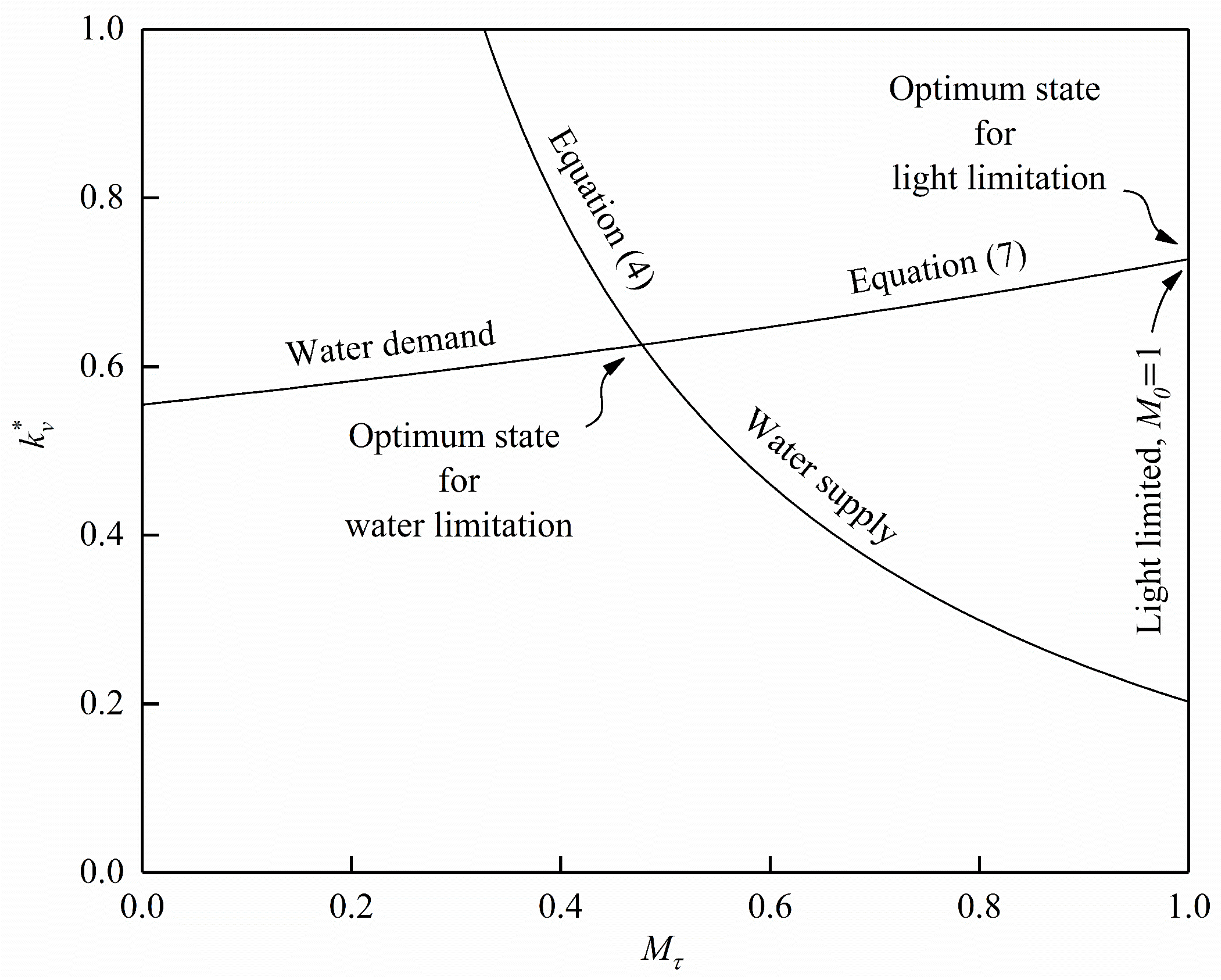
The M 0 required in this research is the vegetation coverage corresponding to the state of maximum productivity in the natural environment during the growing season. This state, also known as the optimum canopy state, must reach the critical moisture state and the optimum foliage state at the same time. Equations (4) and (7) are drawn in Figure 2. If
V e m t b E p s τ 1 + Δ γ 0 1 + Δ γ 0 + ( r c r a ) M = 1 ,
the canopy is light-limited,   k v * = 1 + Δ γ 0 1 + Δ γ 0 + ( r c r a ) M = 1 and its M 0 = 1.
In contrast, if
V e m t b E p s τ < 1 + Δ / γ 0 1 + Δ γ 0 + ( r c r a ) M = 1 ,
the canopy will be water limited, and M 0 is obtained by the simultaneous execution of Equations (4) and (7). At this time, the water supply of the system and the water demand of vegetation reach a dynamic equilibrium.

2.4. Multiple Linear Stepwise Regression Analysis

After checking for correlations between the independent variables, the bidirectional elimination stepwise method was utilized in the multiple linear regression analysis to screen variables and solve the problem of multicollinearity among variables. The bidirectional elimination stepwise method combines forward selection and backward elimination while considering the independent variables one by one [51]. The variance test and the minimum principle of the Akaike information criterion (AIC) were used whether selecting or eliminating variables. Each variable is standardized to obtain standardized partial regression coefficients and thus reflects the linear influence of each independent variable on the dependent variable when other independent variables are fixed.

2.5. Sensitivity Analysis

The relative sensitivity analysis method was used in this study [52,53].
C = i = 0 z 1 | Y i + 1 Y i Y 0 ( F i + 1 F i ) | z ,
where C is the sensitivity coefficient; Y i is the output value of the ith operation of the model;   Y 0 is the output value of the model that inputs the initial parameter value;   F i is the percentage change in the parameter value of the ith operation of the model relative to the initial parameter value; and   z is the number of model runs.

3. Results

3.1. Spatial Distribution and Impact Factors of Observed Vegetation Coverage

The theory of ecohydrological optimality focuses on the long-term average status of the growing season rather than dynamic trends. From the perspective of the spatial distribution, the M value showed horizontal zonal changes, with an average of 0.502 (Figure 3b). The average M values of needleleaf forest, broadleaf forest, scrub, steppe, and cultural vegetation were 0.784 ± 0.176, 0.593 ± 0.241, 0.691 ± 0.212, 0.501 ± 0.171, and 0.456 ± 0.139, respectively, in the 19-year growing season. There was a gradual decrease in M from the eastern edge of the mountainous area to the central section. The plain area is mainly planted with cultural vegetation, which has low vegetation cover.
The correlation of eight meteorological variables was analyzed and then the highly correlated variables were manually removed (here, high correlation means that the correlation coefficient is higher than 0.80 and the results of correlation can be found in the “Supplementary Materials”). We found that the number of independent storms ( m υ ), the mean time between storms ( m t b ), and the mean daily air temperature ( T τ ) were highly correlated except steppe. m υ and T τ were thus excluded due to our primary focus being the response of vegetation to available water during the average interstorm period. Next, the bidirectional elimination multiple linear stepwise regression was used to analyze the influence of meteorological variables on the average growing season M for the five vegetation types from 2000 to 2018 (Table 3). The standardized partial regression coefficient results suggest that the M values of all the vegetation types were significantly affected by the mean storm depth ( m h ), the mean storm duration ( m t r ), and m t b , of which m h is the most significant variable. For the needleleaf forest, the M value was only significantly affected by the precipitation characteristic factors. For the other vegetation types, the mean daily wind speed ( μ ) and the mean daily relative humidity ( R H ) are also important to the M value. It is worth noting that the M value of the steppe was negatively correlated with T τ . Generally, the associations between the precipitation characteristic factors and the M value are stronger than other variables and the M value on a long-term average time scale.

3.2. Verification of Ecohydrological Optimality Theory

To verify the theory of ecohydrological optimality, the k v * value corresponding to the actual vegetation coverage is obtained by inputting the M data into Equation (7). Then, the k v * and M values are substituted into Equation (4) and combined with the water balance equation to obtain the simulated ET. Figure 4a,b presents similar spatial distributions of the average simulated ET data and average observed ET data during the growing season from 2000 to 2018. The simulation results and the observation results are drawn in the scatter plot and fitted by a linear function. As illustrated in Figure 4d, the Nash–Sutcliffe efficiency coefficient (NSE) and the coefficient of determination (R2) demonstrate that the ecohydrological optimality theory is applicable to this watershed in general, with the NSE value being 0.316 and the R2 value being 0.770.
Interestingly, the slope and intercept of the linear function are 1.300 ± 0.003 and −43.084 ± 0.729, respectively. The simulated ET is slightly higher than the observed ET. With successive increases in the observed ET, the degree of deviation of the simulated ET increases. The root mean square error (RMSE) of the scatter plot is 58.280, which indicates that there are marked differences between the simulated ET and the observed ET in some areas. The spatial distribution of these differences is provided in Figure 4c. Compared with the vegetation type distribution (Figure 1b), it can be seen that vegetation types with large differences between the simulated ET and the observed ET are forest (including needleleaf forest and broadleaf forest) and scrub, with high vegetation coverage.

3.3. Simulated Vegetation Coverage Based on the Ecohydrological Optimality Model

The simulated M 0 under the natural environment that a specific climate and soil can maintain was calculated based upon the meteorological, soil, and vegetation data of the watershed for 19 years, with an average of 0.475 (Figure 3a, 2000–2018). The average M 0 values of needleleaf forest, broadleaf forest, scrub, steppe, and cultural vegetation in the growing season were 0.433 ± 0.066, 0.395 ± 0.089, 0.498 ± 0.090, 0.548 ± 0.116, and 0.458 ± 0.100, respectively, from 2000 to 2018. The simulated values were highest in the north and east of the study area and lowest in the central and southwest regions, where the simulated values were roughly similar to the observed values. M exhibited a wide range, from 0.058 to 1, while M 0 exhibited a range from 0.212 to 0.949. The differences between the M and M 0 values increase from the northwest to the southeast of this area, with a maximum value exceeding 0.3 (Figure 3c).

3.4. Sensitivity of the Ideal Vegetation Coverage to the Input Data of the Model

The input parameters of this model were divided into physical parameters ( m h , m v , m t r , m t b , T τ , μ , R H , N , P d , E p s d , L t , M d ) and empirical parameters ( β , h s / h , η 0 , m , n , n e , d , ψ ( 1 ) ,   K ( 1 ) , m s ). The relative sensitivity analysis method facilitated the screening of insensitive parameters in the model. Therefore, the efficiency of the model operation and validation will be improved. When the absolute value of C was less than 0.05, the parameters were considered insensitive and are not shown in Figure 5. The M 0 was not sensitive to soil conditions if the whole watershed was simulated as sandy loam soil (Figure 5a). However, the results of the model were sensitive to all parameters if the soil texture was loam (Figure 5b). When the soil texture was simulated as loamy clay, clay loam, or sandy clay loam, the outputs were sensitive to only effective saturated hydraulic conductivity of soil ( K ( 1 ) ) among all soil parameters (Figure 5c). In all situations, L t was an insensitive parameter, which implied that it may be displaced by an empirical value in future research. Remarkably, the reason the C value of the stem fraction ( h s / h ) of the steppe could not be calculated by this method is that the initial value of this parameter was 0.00. Taken together, these results indicated that the accuracy of meteorological data primarily affected the model results.
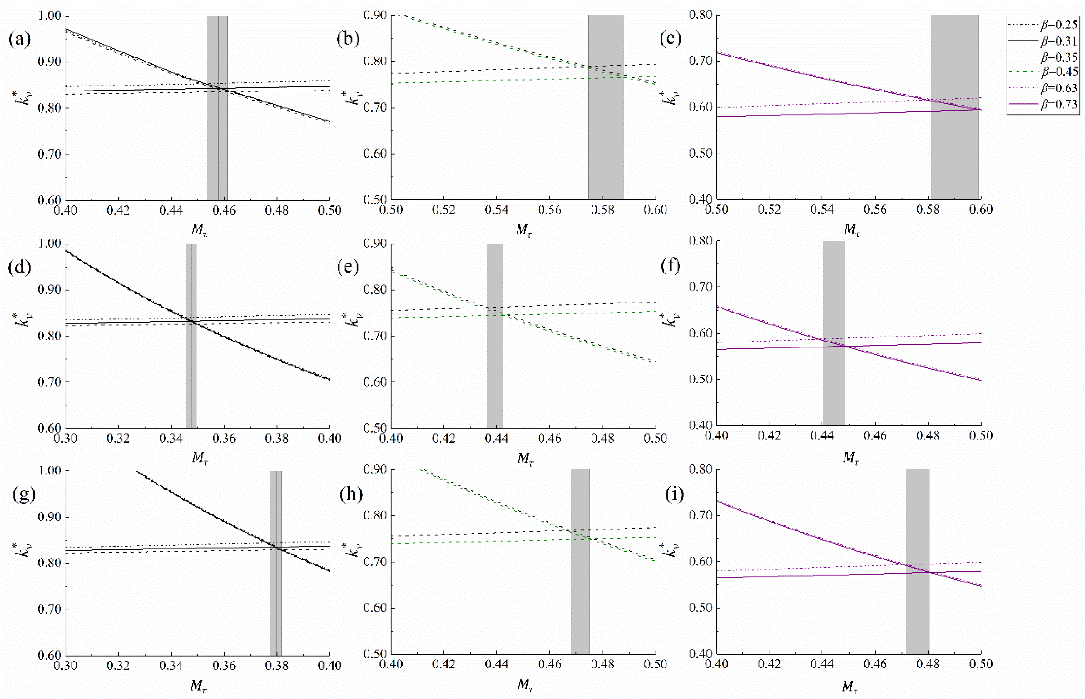
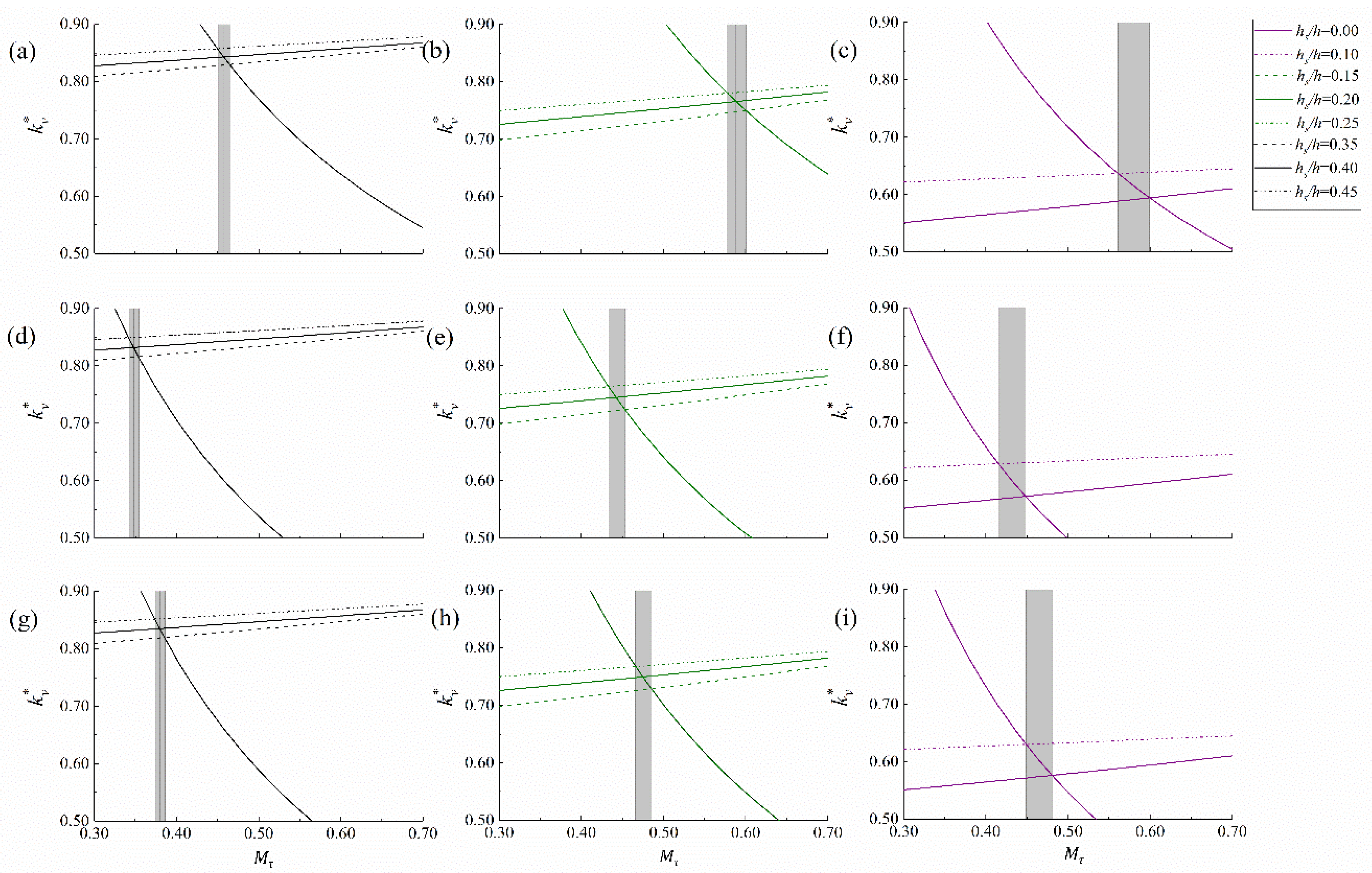
The relative sensitivity analysis method can only qualitatively analyze the input parameters and produce the relative sensitivity ranking of the model parameters. To compare the sensitivities of M 0 at disparate vegetation and soil texture types to the same parameter, further quantitative analysis is needed in accordance with the actual range of the parameters. The observed range of parameters β and h s / h came from previous studies [41,42,46]. As shown in Figure 6 and Figure 7, the variation range of M 0 is quite narrow when β and h s / h change in terms of their actual range. M 0 increases with increasing β or decreasing h s / h . In addition, the change in parameter h s / h changes only the water demand curve, which has nothing to do with soil properties. The results illustrated that the sensitivity of parameter h s / h is affected by only vegetation type, and the sensitivity of parameter β is mainly affected by soil texture. M 0 is more sensitive to β when the soil texture of the study area is simulated as sandy loam instead of other types. The M 0 of the steppe is more sensitive to h s / h than that of the other types.
To shed more light on the response of M 0 to changes in meteorological factors, it is necessary to determine the threshold values of these factors over the years. Obviously, the m h , m t b , and T τ values have a great influence on the M 0 value (Figure 5). M 0 increases as m h increases and m t b and T τ decrease (Figure 8). When the parameter m h changes in the same range, the variation value of M 0 for sandy loam soil is almost twice that for other soil types. Meanwhile, the M 0 of steppe changes more than that of scrub and broadleaf forest. When the parameter m t b changes in the same range, the fluctuation of M 0 for scrub is slightly larger than that for steppe and broadleaf forest. The response ranges of dissimilar vegetation types to temperature sorted by size are steppe, scrub, and broadleaf forest. In summary, the response of M 0 to meteorological factors fluctuates most intensively if the soil type is sandy loam. m h and T τ strongly affected the M 0 of the steppe, and the change in m t b had the greatest influence on the M 0 of scrub.

4. Discussion

In this study, we analyzed the relationship between meteorological factors and the vegetation distribution pattern, evaluated the applicability of the ecohydrological optimality theory in the Yongding River watershed, and calculated the M 0 value in this area based on the local climatic–soil–vegetation conditions. Our observations showed that M had the greatest correlation with the precipitation characteristic factors. The annual average M value in the growing season generally showed horizontal zonal changes. Compared with the simulated M 0 values, there were several differences between M 0 and M in some areas. To use the model more conveniently, we analyzed the sensitivity of the input parameters as well. Collectively, our results indicate that the ecohydrological optimality model is suitable to simulate M 0 in this watershed, and these results could provide reference indicators for ecological restoration.

4.1. Causes for the Distribution Pattern of Vegetation

A large number of studies have shown that vegetation coverage is affected by human activities, precipitation, temperature, and soil moisture conditions [54,55,56]. Analysis of M and meteorological factors enables us to speculate the causes of the distribution pattern of vegetation. Hydrothermal conditions directly affect the spatial distribution of M [57]. On the one hand, increases in the air temperature and radiation will increase evaporation rates, resulting in drier soils, which impede the growth of vegetation [58]. On the other hand, increases in the air temperature and radiation promote photosynthesis, which accelerates the increase in vegetation cover [59]. The steppe was negatively correlated with T τ , possibly because increases in T τ affect the shallow root community in areas such as the steppe to absorb water from the surface of the soil. The heat conditions of the study area are sufficient for steppe growth, which could not offset the negative effect of soil drying [60]. Secondly, the distinct effects of meteorological factors on the vegetation distribution pattern are associated with the vegetation type [61,62]. The mean sunshine duration per day ( N ) and μ significantly affected the broadleaf forest, but not the needleleaf forest. Changes in the needleleaf forest are more dependent on precipitation than ET due to their smaller leaf area and thicker leaf blade, which prevents heat accumulation and water evaporation on the leaf surface [63]. In addition, the variability in the precipitation characteristic factors, especially m h and m t b , changes the spatiotemporal availability of soil water uptake by plants and has a significant impact on vegetation [64]. Zhang [65] found that the number of rainy days, heavy-rainfall events, and consecutive dry days are three important indicators affecting the NDVI in the growing season across the Sahel. Although the multiple stepwise regression quantified the linear impact of the meteorological variables on M , further mathematical and physical deduction is needed for mechanism analysis.
Geographical factors indirectly affect the spatial distribution of M [61,66]. Eastern and southeastern China face the Pacific Ocean, and the amounts of precipitation and humidity decrease from southeast to northwest. Nevertheless, a part of the Tai-hang Mountains is located on the southeast edge of the mountainous area of the Yongding River watershed. The high-altitude mountains influence the distribution of not only hydrothermal conditions but also soil moisture and nutrient conditions [67]. As a consequence, the M of the southeast slope is higher than that of the northwest slope of the Tai-hang Mountains.
Furthermore, the average M value of the steppe and cultural vegetation was lower than that of the other vegetation types in the growing season. This difference may be related to human activities and the drought escape mechanism of vegetation [68]. Because of the undeveloped xylem, herbaceous plants have a low water storage capacity and are sensitive to climate change [69]. Some plants will complete their life cycle ahead of water deficits [70]. Some types of cultural vegetation have the ability to avoid drought by delaying ripening [71]. In addition, this difference is also related to the calculation principle of NDVI. The chlorophyll content and the photosynthetic capacity of the forest were greater than those of the steppe, reflecting the presence of less visible red light, more near infrared light, and a higher NDVI.

4.2. Applicability of the Ecohydrological Optimality Theory

We introduced the MOD16A2 products from NASA to validate the theory. The MOD16A2 data have been verified by the observed latent heat flux from 232 global watersheds and 46 field-based eddy covariance flux towers, and the results, the observed ET, should be considered robust [72]. The annual average M value (Figure 3b) in the growing season is the value obtained under actual local water supply conditions, which is the performance of actual water consumption of vegetation. Similarly, the simulated ET was calculated under the same conditions based on the ecohydrological optimality theory. Consequently, the results presented here can be used to demonstrate the applicability of this theory for cultural vegetation and other types of vegetation (Figure 4). Our findings are consistent with those of Zhang [42]. Conversely, the water supply condition calculated by the water balance equation is under a natural environment without interference (Figure 3a). The simulated M 0 obtained by the model is an ideal value. The correlation between it and the M may be interfered with by human beings.
One unanticipated finding was that the average simulated ET calculated by substituting M in the model was higher than the average observed ET in the region with forest and scrub during the growing season for 19 years. This result implies that the vegetation did not reduce M to avoid water stress but did reduce the transpiration amount in these areas on the scale of 19 years. In other words, this result contradicts the hypothesis that transpiration always occurs at the rate without stress until the vegetation is under initial stress just at the end of the average growing season. Kerkhoff [43] proposed that this seems to be a critical oversight that can cause the transpiration simulated by models to exceed the amount of water available to vegetation. This phenomenon may be related to the simulation process in which the actual situation is replaced by the long-term average value. In a short period of time (within one drought episode), for both trees and herbaceous plants, physiological regulation, such as adjusting the stomata to cope with the situation that the soil moisture is not enough to maintain the maximum transpiration rate in the later interstorm period, will occur in vegetation [73,74]. However, for long time scales, the selection pressure of productivity and the competitive pressure for water allow the types of vegetation that close the stomata much later to survive [75]. Diversified vegetation has different feedback on the frequency of stomatal closure. Most herbaceous plants cannot tolerate premature stomatal closure or frequent stomatal closure, and thus a low vegetation coverage is selected to reduce the demand for water. On the contrary, some woody plants can tolerate or avoid intermittent short-term perturbations of water stress and thereby prevent reductions in vegetation coverage [76,77]. Specifically, longleaf pine responds to extreme drought by better controlling its stomata to limit water loss, and transpiration recovers rapidly during the next precipitation event [78]. The leaves of Robinia pseudoacacia increase the elasticity of the cell wall and veins and the stomatal density to adapt to long-term water stress [15]. Obviously, this long-term, frequent resistance of woody plants to water stress was not considered by Eagleson. Therefore, the M 0 value calculated by ecohydrological optimality theory may be lower than the M value in some areas of forest and scrub, mainly in areas with a high vegetation coverage.
In the long run, the optimal vegetation coverage proposed in this paper is not the maximum vegetation coverage under the same water supply conditions, but the vegetation coverage obtained by minimizing water stress and maximizing productivity. Although trees can tolerate a certain frequency of hydraulic failure, such events may cause embolism in the xylem or roots [79]. The mechanism of drought tolerance or drought avoidance of trees will gradually degenerate as the number of droughts increases [80]. Some research has pointed out that decreases in hydraulic function and photosynthesis for long durations may increase the risk of death after many years [81]. In summary, ecohydrological optimality theory proposes a kind of vegetation coverage that can maintain ecosystem stability.

4.3. Comparison between Simulated and Observed Vegetation Coverage

Our results indicated that the growth of vegetation in this watershed under a natural environment was limited by water, not light, because M 0 < 1. The comparison of M 0 and M contributes to the more effective development of ecological restoration measures. The simulated M 0 was calculated according to the local hydrological cycle, without considering the artificial water supply and consumption. Although built-up lands with intense human activity were not the focus of this research, artificial irrigation, planting, or fertilization of both forest land and farmland occur locally. This condition is one of the reasons M is larger than the simulated M 0 in some areas. In addition, we found that the simulated values along the southeastern edge of the study area were not as high as the observed values. This difference may be caused by the shortage in the number and uneven distribution of meteorological stations, which fails to simulate the actual differences in the hydrothermal distribution due to the impacts of topography. Interpolation of meteorological stations also means that the simulated values are not as detailed as the observed values for the description of the dynamic distribution of vegetation. In general, combined with Figure 4c, when M is obviously larger than M 0 and the observed ET is similar to the simulated ET, it implies that the vegetation has an extra water supply or artificial cultivation and is not under water stress. However, if M is clearly larger than M 0 and the simulated ET is much larger than the observed ET, regardless of whether or not there is extra water supply, the vegetation will suffer from water stress and evolve drought resistance measures.
In the practical process of ecological restoration, we should pay more attention to the quality of vegetation rather than pursue high vegetation coverage. Vegetation restoration should be carried out as the water capacity permits. Excessive vegetation restoration not only keeps vegetation under water stress but also threatens water resources. As the limit of vegetation restoration, M 0 should be classified and discussed in this region. Most needleleaf forests and broadleaf forests in this region have reached M 0 . At this time, we should strengthen the management and protection of existing trees and adopt measures such as forest tending, pruning, and thinning to ensure the growth quality of vegetation [80]. For cultural vegetation, we should use water-saving irrigation technologies and adjust the structure of agricultural planting. For the steppe, we should use fencing and strengthen management measures to ensure natural growth [82].

4.4. Sensitivity of the Ideal Vegetation Coverage to Meteorological, Soil, and Vegetation Factors

Diverse vegetation types and soil texture should be discussed separately in sensitivity analyses because the vegetation and soil parameters are set to different values derived from the actual situation of each grid cell when the model runs. The soil texture mainly affects surface runoff, which results in the distinction of the water available for vegetation. Vegetation type primarily affects the water demand capacity of vegetation. The results demonstrated that the ideal coverage of vegetation planted in sandy loam soil is highly sensitive to changes in meteorological and vegetation factors. This result could be attributed to the runoff calculated from soil properties being extremely small and more water being supplied to the vegetation in this case; thus, soil properties have little effect on the model. The variation in β changed both the water supply curve and the water demand curve. The less surface runoff there is, the more important the surface retention capacity determined by β is. The higher the value of β is, the lower the value of the water demand curve.
These findings suggest that it is better to measure the soil parameters on site if the soil texture is loam or utilize weather stations with high precision to measure the meteorological factors if the soil texture is sandy loam to improve the accuracy of simulations. In addition, scrub vegetation with larger β and smaller h s / h values should be considered in place of forests that are under water stress to increase the vegetation coverage or save water resources.

5. Conclusions

On a long-term average timescale, the optimal coverage of vegetation in the Yongding River watershed is limited by water rather than light. In this study, the spatial patterns and impact factors of vegetation were explored at the watershed scale. Meanwhile, we verified the applicability of the ecohydrological optimality theory in this region and calculated the M 0 value in terms of the local meteorological, soil, and vegetation factors from 2000 to 2018. Finally, the sensitivity of M 0 to the input parameters of the model under disparate conditions of vegetation and soil was also considered. Additionally, a large number of studies with long-term observations of precipitation, runoff, transpiration, soil moisture, and root depth of vegetation are needed in future work. The main findings obtained from this research are as follows:
  • From the spatial point of view, the holistic M exhibits horizontal zonal changes that basically correspond to topographic factors, which gradually decrease from the eastern edge of the mountainous area to the central section. Temperature increases limited the water needed by the steppe. The m h , m t r , and m t b values had the highest correlation with the M value, as they controlled the spatial and temporal distribution of the water available for vegetation.
  • The ecohydrological optimality model simulates a kind of vegetation coverage that maximizes the productivity of biomass in the absence of water stress rather than the maximum vegetation coverage, as this model cannot completely simulate the adaptive strategies of vegetation to water stress. The vegetation coverage proposed by ecohydrological optimality theory can reduce the risk of embolism in the xylem or roots or vegetation death in the years following drought events, which is significant for maintaining the stability of ecosystems.
  • The M 0 should be used as the limit of vegetation restoration, regardless of whether the vegetation evolves drought resistance measures. For forests that have reached M 0 , we should strengthen the management and improve the quality of existing vegetation. For cultural vegetation that has not reached the M 0 value, we should use water-saving irrigation technologies and adjust the structure of agricultural planting. For the steppe, we should use fencing and strengthen management measures to ensure natural growth.
  • In this model, the accuracy of meteorological data is essential. The M 0 value was the most sensitive to the meteorological factors and β when the soil texture of the study area was simulated as sandy loam instead of the other types. The M 0 of the steppe is most sensitive to h s / h , m h , and T τ .

Supplementary Materials

The following are available online at https://www.mdpi.com/article/10.3390/f12101377/s1, Table S1: Correlation coefficients between the meteorological variables for needleleaf forest, Table S2: Correlation coefficients between the meteorological variables for broadleaf forest, Table S3: Correlation coefficients between the meteorological variables for scrub, Table S4: Correlation coefficients between the meteorological variables for steppe, and Table S5: Correlation coefficients between the meteorological variables for cultural vegetation.

Author Contributions

Conceptualization, Y.Z. and T.Z.; methodology, Y.Z. and C.S.; software, Y.Z.; validation, Y.Z. and T.Z.; formal analysis, Y.Z.; investigation, Y.Z. and Q.M.; resources, Q.M.; data curation, Y.Z. and Q.M.; writing—original draft preparation, Y.Z.; writing—review and editing, T.Z.; visualization, Y.Z.; supervision, C.S.; project administration, C.S.; funding acquisition, T.Z. All authors have read and agreed to the published version of the manuscript.

Funding

This research was funded by the entrusted project of the Beijing Gardening and Greening Bureau, China (the project title is Monitoring and Evaluation of Ecological Benefits of Cooperative Afforestation Project between Beijing and Hebei Province in 2018), grant number 2018HXFWSBXY029.

Institutional Review Board Statement

Not applicable.

Informed Consent Statement

Not applicable.

Data Availability Statement

Publicly available datasets were analyzed in this study and their websites are provided in the Section 2 “Materials and Methods”.

Acknowledgments

Acknowledgements for the data support from the China Meteorological Data Service Center (http://data.cma.cn accessed on 5 October 2019), the Geospatial Data Cloud site, Computer Network Information Center, Chinese Academy of Sciences (http://www.gscloud.cn accessed on 1 December 2009), the Data Center for Resources and Environmental Sciences, Chinese Academy of Sciences (RESDC) (http://www.resdc.cn accessed on 30 May 2001), the NASA EARTHDATA (https://earthdata.nasa.gov/ accessed on 1 April 2020), and the website of Ministry of Water Resources of the People’s Republic of China (http://www.mwr.gov.cn/ accessed on 29 January 2019).

Conflicts of Interest

The authors declare no conflict of interest.

Appendix A. Assumptions of the Theory of Ecohydrological Optimality

In the theory of ecohydrological optimality, the natural environment refers to ideal conditions that are not irrigated, cultivated, or artificially fertilized. Vegetation is not affected by human-made factors or natural disasters. Water and light are the only limiting factors of vegetation, while nutrients and CO2 (carbon dioxide) are infinite. In addition, the groundwater level in the study area is sufficiently deep, which is according to the premise of the assumption that all surface runoff was “Hortonian” [83].

Appendix B. Supplementary Formula

The term of precipitation in Equation (2) described by Eagleson is
P τ = m υ m h ,
where P τ is the precipitation in the growing season, mm. The probability density functions of the storm depth, h , were expressed as incomplete gamma. Hence,   m h = κ 0 / λ 0 , in which κ 0 is the shape parameter of the gamma distribution, dimensionless; λ 0 is the scale parameter of the gamma distribution, mm−1. The precipitation characteristic parameters also have the storm duration,   t r , the time between storms,  t b , and the storm intensity,   i . These parameters were all assumed to be exponentially distributed, with m t r = 1 / δ , m t b = 1 / α and m i = 1 / ω , where δ , α , and ω aret eh exponential distribution rate parameters of precipitation characteristic parameters.
The capillary rise from the water table is expressed as
m τ w = m τ K ( 1 ) [ 1 + 3 / 2 m s c 1 ] [ Ψ ( 1 ) z w ] m s c ,
where c is the permeability index of soil, dimensionless; and z w is the depth to the water table, mm.
Eagleson assumed that the surface retention of each independent storm is evaporated during the subsequent interstorm period. The temporal average storm surface retention is estimated by
E [ E r ] ( 1 + M τ η 0 β L t ) h 0 ,
where h 0 is the storm retention depth on all surfaces, mm, with a constant nominal value of 1. The available values of LAI were used as the first approximation to L t .
When i and t r are assumed to be independent random variables, the expected value of the R s j is obtained by
E [ R s j ] = m h [ ( 1 M τ ) e G ( 0 ) 2 σ ( 0 ) 3 2 + M τ e 2 G ( 0 ) ] ,
where G ( 0 ) is the gravitational infiltration parameter, dimensionless, and σ ( 0 ) is the capillary infiltration parameter, dimensionless. They can be further expressed as
G ( 0 ) ω K ( 1 ) 2 ,
σ ( 0 ) [ 5 n e λ 2 K ( 1 ) ψ ( 1 ) ϕ i ( d , 0 ) 6 π δ m s κ 0 2 ] 1 3 ,
in which ϕ i ( d , 0 ) is the sorption diffusivity, expressed as ϕ i ( d , 0 ) = 1 d + 5 / 3 , dimensionless.
The percolation of soil water is
m τ v = m τ K ( 1 ) s 0 c ,
where s 0 is the spatiotemporal average soil moisture concentration in the root zone, dimensionless.
The last term of Equation (2) is
Δ S = [ P d ( 1 M d ) E p s d m d Y d ]
where Y d is the long-term average water yield of the nongrowing season, mm, which is assumed to be 0.
In Equation (3),
m t b = m t b η 0 β L t h 0 2 E p s τ ,
m t b = m t b h 0 E p s τ
The capillary rise from the water table, the percolation of soil water, and bare soil evaporation were ignored in this article. According to Equations (2)–(4), it can be calculated that,
V e m h [ 1 ( 1 + M τ η 0 β L t ) h 0 m h ( 1 M τ ) e G ( 0 ) 2 σ ( 0 ) 3 2 M τ e 2 G ( 0 ) Δ S m υ m h ]
In Equation (7), the resistance ratio for open canopies simplifies to
( r c r a ) M 0 1 h s / h 0.33 + h s / h
The resistance ratio for closed canopies is
n s ( r c r a ) M = 1 = ( 1 m m ) ( γ L t ) 2 ( L t 1 ) ( 1 e 1 m m γ L t ) [ 0.577 + ln ( L t 1 ) + 1 2 ( L t 1 ) 1 ] ,
where n s is the ratio of the stomated leaf area to the projected leaf area, whose value is 1 in this study, dimensionless; γ is the extinction parameter for horizontal wind velocity,   γ m n β , dimensionless; and L t is the foliage area index for closed canopies.

References

  1. Rodriguez-Iturbe, I.; Porporato, A. Ecohydrology of Water-Controlled Ecosystems: Soil Moisture and Plant Dynamics; Cambridge University Press: New York, NY, USA, 2004. [Google Scholar]
  2. Wang, X.J.; Zhang, B.Q.; Xu, X.F.; Tian, J.; He, C.S. Regional water-energy cycle response to land use/cover change in the agropastoral ecotone, northwest China. J. Hydrol. 2020, 580, 124246. [Google Scholar] [CrossRef]
  3. Tian, S.Y.; Renzullo, L.J.; van Dijk, A.I.J.M.; Tregoning, P.; Walker, J.P. Global joint assimilation of GRACE and SMOS for improved estimation of root-zone soil moisture and vegetation response. Hydrol. Earth Syst. Sci. 2019, 23, 1067–1081. [Google Scholar] [CrossRef] [Green Version]
  4. Xu, X.Y.; Yang, D.W.; Sivapalan, M. Assessing the impact of climate variability on catchment water balance and vegetation cover. Hydrol. Earth Syst. Sci. 2012, 16, 43–58. [Google Scholar] [CrossRef] [Green Version]
  5. Zhang, X.Y.; Zhang, B.Q. The responses of natural vegetation dynamics to drought during the growing season across China. J. Hydrol. 2019, 574, 706–714. [Google Scholar] [CrossRef]
  6. Weltzin, J.F.; Loik, M.E.; Susanne, S.; Williams, D.G.; Fay, P.A.; Haddad, B.M.; John, H.; Huxman, T.E.; Knapp, A.K.; Guanghui, L. Assessing the response of terrestrial ecosystems to potential changes in precipitation. Bioscience 2003, 53, 941–952. [Google Scholar] [CrossRef]
  7. Noy-Meir, I. Desert ecosystems: Environment and producers. Annu. Rev. Ecol. Syst. 1973, 4, 25–51. [Google Scholar] [CrossRef]
  8. Vicente-Serrano, S.M.; Gouveia, C.; Camarero, J.J.; Begueria, S.; Trigo, R.; Lopez-Moreno, J.I.; Azorin-Molina, C.; Pasho, E.; Lorenzo-Lacruz, J.; Revuelto, J.; et al. Response of vegetation to drought time-scales across global land biomes. Proc. Natl. Acad. Sci. USA 2013, 110, 52–57. [Google Scholar] [CrossRef] [Green Version]
  9. Brady, N.C.; Weil, R.R. The Nature and Properties of Soils, 8th ed.; Macmillan Publishers: New York, NY, USA, 1974. [Google Scholar]
  10. Osman, K.T. Physical properties of forest soils. In Forest Soils: Properties and Management; Springer International Publishing: Heidelberg, Germany, 2013; pp. 19–44. [Google Scholar]
  11. Eagleson, P.S. Ecological optimality in water-limited natural soil-vegetation systems: 1. Theory and hypothesis. Water Resour. Res. 1982, 18, 325–340. [Google Scholar] [CrossRef] [Green Version]
  12. Chaves, M.M.; Maroco, J.P.; Pereira, J.S. Understanding plant responses to drought—From genes to the whole plant. Funct. Plant Biol. 2003, 30, 239–264. [Google Scholar] [CrossRef]
  13. Ding, Y.B.; Xu, J.T.; Wang, X.W.; Peng, X.B.; Cai, H.J. Spatial and temporal effects of drought on Chinese vegetation under different coverage levels. Sci. Total Environ. 2020, 716, 137166. [Google Scholar] [CrossRef]
  14. Volaire, F. A unified framework of plant adaptive strategies to drought: Crossing scales and disciplines. Global Chang. Biol. 2018, 24, 2929–2938. [Google Scholar] [CrossRef] [Green Version]
  15. Zhang, Z.; Huang, M.; Zhao, X.; Wu, L. Adjustments of leaf traits and whole plant leaf area for balancing water supply and demand in Robinia pseudoacacia under different precipitation conditions on the Loess Plateau. Agric. For. Meteorol. 2019, 279, 107733. [Google Scholar] [CrossRef]
  16. Xu, H.J.; Wang, X.P.; Zhao, C.Y.; Yang, X.M. Diverse responses of vegetation growth to meteorological drought across climate zones and land biomes in northern China from 1981 to 2014. Agric. For. Meteorol. 2018, 262, 1–13. [Google Scholar] [CrossRef]
  17. Anderegg, L.; Hillerislambers, J. Drought stress limits the geographic ranges of two tree species via different physiological mechanisms. Glob. Chang. Biol. 2016, 22, 1029–1045. [Google Scholar] [CrossRef] [PubMed]
  18. Kijowska-Oberc, J.; Staszak, A.M.; Kamiński, J.; Ratajczak, E. Adaptation of forest trees to rapidly changing climate. Forests 2020, 11, 123. [Google Scholar] [CrossRef] [Green Version]
  19. Givnish, T.J. Adaptation to sun and shade: A whole-plant perspective. Aust. J. Plant Physiol. 1988, 15, 63–92. [Google Scholar] [CrossRef] [Green Version]
  20. Caylor, K.K.; Scanlon, T.M.; Rodriguez-Iturbe, I. Feasible optimality of vegetation patterns in river basins. Geophys. Res. Lett. 2004, 31, 1–4. [Google Scholar] [CrossRef] [Green Version]
  21. Wang, Y.J.; Sperry, J.S.; Anderegg, W.R.L.; Venturas, M.D.; Trugman, A.T. A theoretical and empirical assessment of stomatal optimization modeling. New Phytol. 2020, 227, 311–325. [Google Scholar] [CrossRef] [Green Version]
  22. Eagleson, P.S.; Tellers, T.E. Ecological optimality in water-limited natural soil-vegetation systems: 2. Tests and applications. Water Resour. Res. 1982, 18, 341–354. [Google Scholar] [CrossRef] [Green Version]
  23. Eagleson, P.S. Ecohydrology: Darwinian Expression of Vegetation Form and Function; Cambridge University Press: Cambridge, UK, 2002. [Google Scholar]
  24. Eagleson, P.S. Dynamics of flood frequency. Water Resour. Res. 1972, 8, 878–898. [Google Scholar] [CrossRef]
  25. Eagleson, P.S. Climate, soil, and vegetation: 1. Introduction to water balance dynamics. Water Resour. Res. 1978, 14, 705–712. [Google Scholar] [CrossRef] [Green Version]
  26. Eagleson, P.S. Climate, soil, and vegetation: 2. The distribution of annual precipitation derived from observed storm sequences. Water Resour. Res. 1978, 14, 713–721. [Google Scholar] [CrossRef] [Green Version]
  27. Eagleson, P.S. Climate, soil, and vegetation: 3. A simplified model of soil moisture movement in the liquid phase. Water Resour. Res. 1978, 14, 722–730. [Google Scholar] [CrossRef] [Green Version]
  28. Eagleson, P.S. Climate, soil, and vegetation: 4. The expected value of annual evapotranspiration. Water Resour. Res. 1978, 14, 731–739. [Google Scholar] [CrossRef] [Green Version]
  29. Eagleson, P.S. Climate, soil, and vegetation: 5. A derived distribution of storm surface runoff. Water Resour. Res. 1978, 14, 741–748. [Google Scholar] [CrossRef] [Green Version]
  30. Eagleson, P.S. Climate, soil, and vegetation: 6. Dynamics of the annual water balance. Water Resour. Res. 1978, 14, 749–764. [Google Scholar] [CrossRef] [Green Version]
  31. Eagleson, P.S. Climate, soil, and vegetation: 7. A derived distribution of annual water yield. Water Resour. Res. 1978, 14, 765–776. [Google Scholar] [CrossRef] [Green Version]
  32. Restrepo-Posada, P.J.; Eagleson, P.S. Identification of independent rainstorms. J. Hydrol. 1982, 55, 303–319. [Google Scholar] [CrossRef]
  33. Entekhabi, D.; Rodriguez-Iturbe, I.; Eagleson, P.S. Probabilistic representation of the temporal rainfall process by a modified Neyman-Scott rectangular pulses model: Parameter estimation and validation. Water Resour. Res. 1989, 25, 295–302. [Google Scholar] [CrossRef] [Green Version]
  34. Guo, Y.P.; Adams, B.J. Hydrologic analysis of urban catchments with event-based probabilistic models: 1. Runoff volume. Water Resour. Res. 1998, 34, 3421–3431. [Google Scholar] [CrossRef]
  35. Guo, Y.P.; Adams, B.J. Hydrologic analysis of urban catchments with event-based probabilistic models: 2. Peak discharge rate. Water Resour. Res. 1998, 34, 3433–3443. [Google Scholar] [CrossRef]
  36. Guo, Y.P.; Liu, S.G.; Baetz, B.W. Probabilistic rainfall-runoff transformation considering both infiltration and saturation excess runoff generation processes. Water Resour. Res. 2012, 48, 1–17. [Google Scholar] [CrossRef] [Green Version]
  37. Kochendorfer, J.P.; Ramirez, J.A. Modeling the monthly mean soil-water balance with a statistical-dynamical ecohydrology model as coupled to a two-component canopy model. Hydrol. Earth Syst. Sci. 2010, 14, 2099–2120. [Google Scholar] [CrossRef]
  38. Salvucci, G.D.; Entekhabi, D. Comparison of the Eagleson statistical-dynamical water balance model with numerical simulations. Water Resour. Res. 1994, 30, 2751–2757. [Google Scholar] [CrossRef]
  39. Rodriguez-Iturbe, I. Ecohydrology: A hydrologic perspective of climate-soil-vegetation dynamies. Water Resour. Res. 2000, 36, 3–9. [Google Scholar] [CrossRef] [Green Version]
  40. Mo, K.L.; Cong, Z.T.; Lei, H.M. Optimal vegetation cover in the Horqin Sands, China. Ecohydrology 2016, 9, 700–711. [Google Scholar] [CrossRef]
  41. Cong, Z.T.; Li, Q.S.; Mo, K.L.; Zhang, L.X.; Shen, H. Ecohydrological optimality in the Northeast China Transect. Hydrol. Earth Syst. Sci. 2017, 21, 2449–2462. [Google Scholar] [CrossRef] [Green Version]
  42. Zhang, S.L.; Yang, D.W.; Yang, Y.T.; Piao, S.L.; Yang, H.B.; Lei, H.M.; Fu, B.J. Excessive afforestation and aoil drying on China’s Loess Plateau. J. Geophys. Res. Biogeosci. 2018, 123, 923–935. [Google Scholar] [CrossRef]
  43. Kerkhoff, A.J.; Martens, S.N.; Milne, B.T. An ecological evaluation of Eagleson’s optimality hypotheses. Funct. Ecol. 2004, 18, 404–413. [Google Scholar] [CrossRef]
  44. Li, M.M.; Wu, B.F.; Yan, C.Z.; Zhou, W.F. Estimation of vegetation fraction in the upper basin of Miyun reservoir by remote sensing. Resour. Sci. 2004, 26, 153–159. [Google Scholar] [CrossRef]
  45. Allen, R.G.; Pereira, L.S.; Raes, D.; Smith, M. FAO Irrigation and Drainage Paper; Food and Agriculture Organization of the United Nations: Rome, Italy, 1998. [Google Scholar]
  46. Rauner, J.L. Deciduous forests. In Vegetation and the Atmosphere; Academic Press: New York, NY, USA, 1976; Volume 2, pp. 241–264. [Google Scholar]
  47. Ripley, E.A.; Redmann, R.E. Grassland. In Vegetation and the Atmosphere; Academic Press: New York, NY, USA, 1976; Volume 2. [Google Scholar]
  48. Waring, R.H. Estimating forest growth and efficiency in relation to canopy leaf area. Adv. Ecol. Res. 1983, 13, 327–354. [Google Scholar] [CrossRef]
  49. Amiro, B.D. Drag coefficients and turbulence spectra within three boreal forest anopies. Bound.-Lay Meteorol. 1990, 52, 227–246. [Google Scholar] [CrossRef]
  50. Horn, H.S. The Adaptive Geometry of Trees; Princeton University Press: Princeton, NJ, USA, 1971. [Google Scholar]
  51. Afantitis, A.; Melagraki, G.; Sarimveis, H.; Koutentis, P.A.; Markopoulos, J.; Igglessi-Markopoulou, O. A novel simple QSAR model for the prediction of anti-HIV activity using multiple linear regression analysis. Mol. Divers. 2006, 10, 405–414. [Google Scholar] [CrossRef]
  52. Francos, A.; Elorza, F.J.; Bouraoui, F.; Bidoglio, G.; Galbiati, L. Sensitivity analysis of distributed environmental simulation models: Understanding the model behaviour in hydrological studies at the catchment scale. Reliab. Eng. Syst. Saf. 2003, 79, 205–218. [Google Scholar] [CrossRef]
  53. Gao, Y.H.; Sha, X.J.; Xu, X.Y. Sensitivity analysis of SWMM model parameters based on Morris method. J. Water Res. Water Eng. 2016, 27, 87–90. [Google Scholar] [CrossRef]
  54. Al Balasmeh, O.I.; Karmaker, T. Effect of temperature and precipitation on the vegetation dynamics of high and moderate altitude natural forests in India. J. Indian Soc. Remote 2020, 48, 121–144. [Google Scholar] [CrossRef]
  55. Liu, S.Y.; Huang, S.Z.; Xie, Y.Y.; Wang, H.; Huang, Q.; Leng, G.Y.; Li, P.; Wang, L. Spatial-temporal changes in vegetation cover in a typical semi-humid and semi-arid region in China: Changing patterns, causes and implications. Ecol. Indic. 2019, 98, 462–475. [Google Scholar] [CrossRef]
  56. Yu, X.; Yang, H.B.; Li, S.E.; Yang, D.W. An improved conceptual model quantifying the effect of climate change and anthropogenic activities on vegetation change in arid regions. Remote Sens. 2019, 11, 2110. [Google Scholar] [CrossRef] [Green Version]
  57. Shen, Q.; Gao, G.Y.; Han, F.; Xiao, F.Y.; Ma, Y.; Wang, S.; Fu, B.J. Quantifying the effects of human activities and climate variability on vegetation cover change in a hyper-arid endorheic basin. Land Degrad. Dev. 2018, 29, 3294–3304. [Google Scholar] [CrossRef]
  58. Shaver, G.R.; Canadell, J.; Chapin, F.S.; Gurevitch, J.; Harte, J.; Henry, G.; Ineson, P.; Jonasson, S.; Melillo, J.; Pitelka, L. Global warming and terrestrial ecosystems: A conceptual framework for analysis. Bioscience 2000, 50, 871–882. [Google Scholar] [CrossRef]
  59. Illman, S. Hilbert’s fifth problem: Review. J. Math. Sci. 2001, 105, 1843–1847. [Google Scholar] [CrossRef]
  60. Bao, G.; Bao, Y.H.; Sanjjava, A.; Qin, Z.H.; Zhou, Y.; Xu, G. NDVI-indicated long-term vegetation dynamics in Mongolia and their response to climate change at biome scale. Int. J. Climatol. 2015, 35, 4293–4306. [Google Scholar] [CrossRef]
  61. Chen, Z.F.; Wang, W.G.; Fu, J.Y. Vegetation response to precipitation anomalies under different climatic and biogeographical conditions in China. Sci. Rep. 2020, 10, 830. [Google Scholar] [CrossRef] [PubMed] [Green Version]
  62. Sun, W.Y.; Song, X.Y.; Mu, X.M.; Gao, P.; Wang, F.; Zhao, G.G. Spatiotemporal vegetation cover variations associated with climate change and ecological restoration in the Loess Plateau. Agric. For. Meteorol. 2015, 209, 87–99. [Google Scholar] [CrossRef]
  63. Bhusal, N.; Lee, M.; Han, A.R.; Han, A.; Kim, H.S. Responses to drought stress in Prunus sargentii and Larix kaempferi seedlings using morphological and physiological parameters. For. Ecol. Manag. 2020, 465, 1–12. [Google Scholar] [CrossRef]
  64. Verbruggen, W.; Schurgers, G.; Horion, S.; Ardo, J.; Bernardino, P.N.; Cappelaere, B.; Demarty, J.; Fensholt, R.; Kergoat, L.; Sibret, T.; et al. Contrasting responses of woody and herbaceous vegetation to altered rainfall characteristics in the Sahel. Biogeosciences 2021, 18, 77–93. [Google Scholar] [CrossRef]
  65. Zhang, W.M.; Brandt, M.; Tong, X.Y.; Tian, Q.J.; Fensholt, R. Impacts of the seasonal distribution of rainfall on vegetation productivity across the Sahel. Biogeosciences 2018, 15, 319–330. [Google Scholar] [CrossRef] [Green Version]
  66. Deng, S.F.; Yang, T.B.; Zeng, B.; Zhu, X.F.; Xu, H.J. Vegetation cover variation in the Qilian Mountains and its response to climate change in 2000–2011. J. Mt. Sci. 2013, 10, 1050–1062. [Google Scholar] [CrossRef]
  67. Riihimäki, H.; Heiskanen, J.; Luoto, M. The effect of topography on arctic-alpine aboveground biomass and NDVI patterns. Int. J. Appl. Earth Obs. 2017, 56, 44–53. [Google Scholar] [CrossRef] [Green Version]
  68. Shavrukov, Y.; Kurishbayev, A.; Jatayev, S.; Shvidchenko, V.; Zotova, L.; Koekemoer, F.; De Groot, S.; Soole, K.; Langridge, P. Early flowering as a drought escape mechanism in plants: How can it aid wheat production? Front. Plant Sci. 2017, 8, 1950. [Google Scholar] [CrossRef]
  69. Craine, J.M.; Ocheltree, T.W.; Nippert, J.B.; Towne, E.G.; Skibbe, A.M.; Kembel, S.W.; Fargione, J.E. Global diversity of drought tolerance and grassland climate-change resilience. Nat. Clim. Chang. 2013, 3, 63–67. [Google Scholar] [CrossRef]
  70. Piao, S.L.; Friedlingstein, P.; Ciais, P.; Viovy, N.; Demarty, J. Growing season extension and its impact on terrestrial carbon cycle in the Northern Hemisphere over the past 2 decades. Glob. Biogeochem. Cycles 2007, 21, 3018. [Google Scholar] [CrossRef]
  71. Butterfield, Z.; Buermann, W.; Keppel-Aleks, G. Satellite observations reveal seasonal redistribution of northern ecosystem productivity in response to interannual climate variability. Remote Sens. Environ. 2020, 242, 111755. [Google Scholar] [CrossRef]
  72. Running, S.W.; Mu, Q.Z.; Zhao, M.S.; Moreno, A. MODIS Global Terrestrial Evapotranspiration (ET) Product (MOD16A2/A3 and Year-End Gap-Filled MOD16A2GF/A3GF) NASA Earth Observing System MODIS Land Algorithm (For Collection 6). 2019. Available online: https://modis-land.gsfc.nasa.gov/pdf/MOD16UsersGuideV2.022019.pdf (accessed on 29 January 2019).
  73. Levitt, J. Water, radiation, salt, and other stresses. In Responses of Plants to Environmental Stresses, 2nd ed.; Academic Press: New York, NY, USA, 1980; Volume 2. [Google Scholar]
  74. McDowell, N.; Pockman, W.T.; Allen, C.D.; Breshears, D.D.; Cobb, N.; Kolb, T.; Plaut, J.; Sperry, J.; West, A.; Williams, D.G. Mechanisms of plant survival and mortality during drought: Why do some plants survive while others succumb to drought? New Phytol. 2008, 178, 719–739. [Google Scholar] [CrossRef] [PubMed]
  75. Lu, Y.J.; Duursma, R.A.; Farrior, C.E.; Medlyn, B.E.; Feng, X. Optimal stomatal drought response shaped by competition for water and hydraulic risk can explain plant trait covariation. New Phytol. 2020, 225, 1206–1217. [Google Scholar] [CrossRef]
  76. Moran, E.; Lauder, J.; Musser, C.; Stathos, A.; Shu, M. The genetics of drought tolerance in conifers. New Phytol. 2017, 216, 1034–1048. [Google Scholar] [CrossRef] [Green Version]
  77. Schwarz, J.; Skiadaresis, G.; Kohler, M.; Kunz, J.; Schnabel, F.; Vitali, V.; Bauhus, J. Quantifying growth responses of trees to drought—A critique of commonly used resilience indices and recommendations for future studies. Curr. For. Rep. 2020, 6, 185–200. [Google Scholar] [CrossRef]
  78. Samuelson, L.J.; Stokes, T.A.; Ramirez, M.R.; Mendonca, C.C. Drought tolerance of a Pinus palustris plantation. For. Ecol. Manag. 2019, 451, 117557. [Google Scholar] [CrossRef]
  79. Anderegg, W.R.L.; Plavcova, L.; Anderegg, L.D.L.; Hacke, U.G.; Berry, J.A.; Field, C.B. Drought’s legacy: Multiyear hydraulic deterioration underlies widespread aspen forest die-off and portends increased future risk. Glob. Chang. Biol. 2013, 19, 1188–1196. [Google Scholar] [CrossRef] [PubMed]
  80. Berdanier, A.B.; Clark, J.S. Multiyear drought-induced morbidity preceding tree death in southeastern US forests. Ecol. Appl. 2016, 26, 17–23. [Google Scholar] [CrossRef] [Green Version]
  81. McDowell, N.G.; Williams, A.P.; Xu, C.; Pockman, W.T.; Dickman, L.T.; Sevanto, S.; Pangle, R.; Limousin, J.; Plaut, J.; Mackay, D.S.; et al. Multi-scale predictions of massive conifer mortality due to chronic temperature rise. Nat. Clim. Chang. 2016, 6, 295–300. [Google Scholar] [CrossRef]
  82. Li, Y.R.; Cao, Z.; Long, H.L.; Liu, Y.S.; Li, W.J. Dynamic analysis of ecological environment combined with land cover and NDVI changes and implications for sustainable urban–rural development: The case of Mu Us Sandy Land, China. J. Clean. Prod. 2017, 142, 697–715. [Google Scholar] [CrossRef]
  83. Horton, R.E. The role of infiltration in the hydrologic cycle. Eos Trans. Am. Geophys. Union 1933, 14, 446–460. [Google Scholar] [CrossRef]
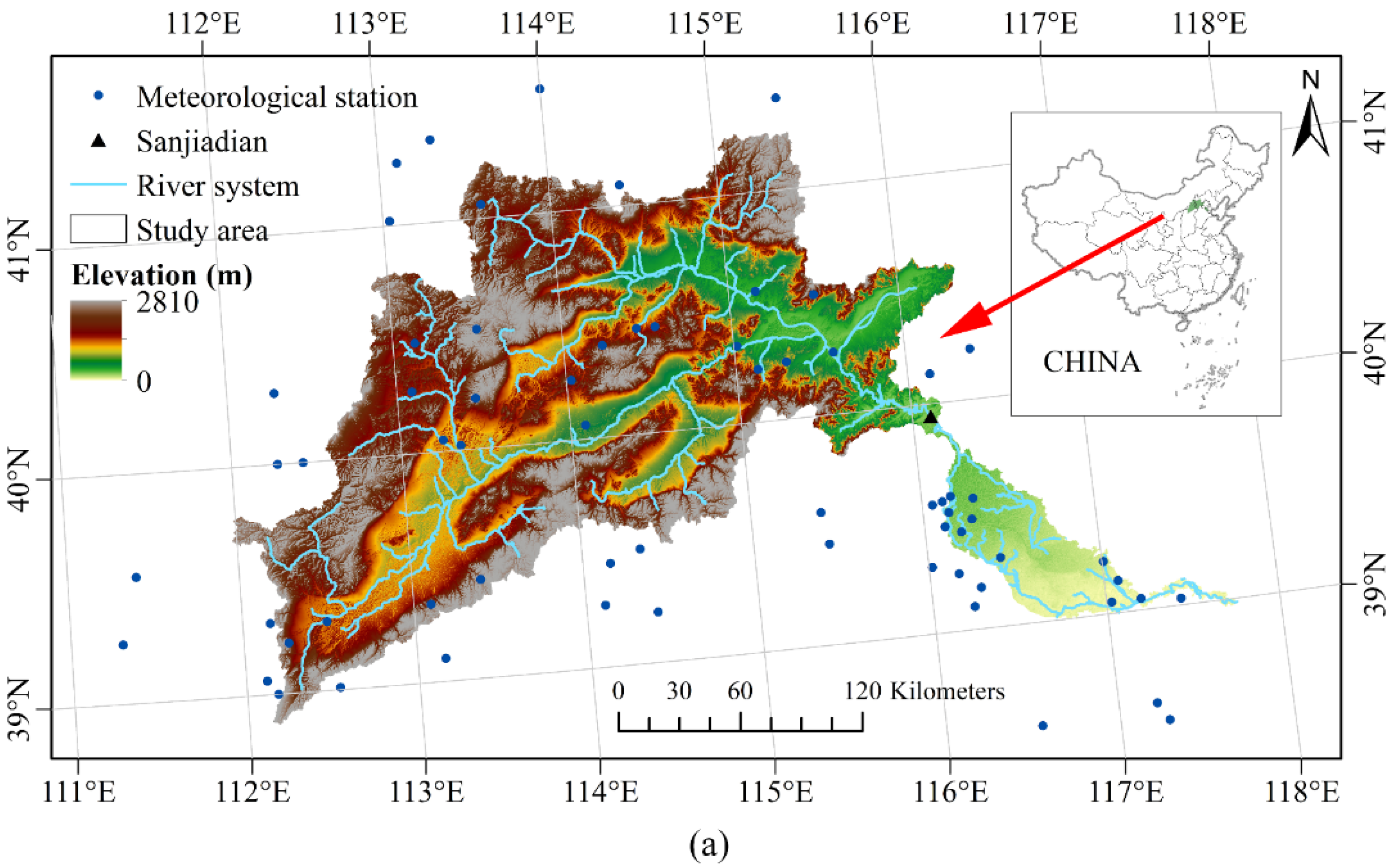
Figure 1. General conditions of the Yongding River watershed, China. (a) Geographic location; (b) major vegetation types; (c) soil texture types. Blank grids in the study area are urban and built-up lands, water bodies, wetlands, or barren areas, which are not included in the research of this paper. The WGS84 geographic coordinate system and Albers projection coordinate system were used. The resolution of (a) is 30 m and that of (b,c) is 1 km.
Forests 12 01377 g001aForests 12 01377 g001b
Figure 2. Optimum canopy state, where M τ is the mean vegetation coverage during growing season, dimensionless; and k v * is the potential canopy conductance, dimensionless [23].
Forests 12 01377 g002
Figure 3. Comparison of the average ideal vegetation coverage ( M 0 ) versus the average M during the growing season from 2000 to 2018. (a) Distribution of M 0 . (b) Distribution of M . (c) Difference between M 0   and M .
Forests 12 01377 g003
Figure 4. Comparison of the average simulated evapotranspiration (ET) versus the average observed ET during the growing season from 2000 to 2018. Spatial distribution of simulated ET in (a); spatial distribution of observed ET in (b); difference between simulated and observed ET in (c); scatterplot of simulated and observed ET in (d), in which the sample capacity was 47690. * represents significance at a level of 0.05.
Forests 12 01377 g004
Figure 5. Sensitivity coefficient distribution of M 0 for diverse vegetation and soil texture types to input parameters. The soil texture of this area is simulated as sandy loam in part (a); the soil texture is simulated as loam soil in part (b); and the soil texture is simulated as loamy clay, clay loam, or sandy clay loam in part (c).
Forests 12 01377 g005
Figure 6. M 0 changed with the cosine of the leaf angle ( β ). In this study, the observed β of broadleaf forest ranged from 0.25 to 0.35 with an original value of 0.31 in the model; the observed β of scrub ranged from 0.35 to 0.45 with an original value of 0.45, and the observed β of steppe ranged from 0.63 to 0.73 with an original value of 0.73. The intersection of the auxiliary vertical line and abscissa is M 0 . Vegetation types and soil texture types: (a,d,g) Broadleaf forest; (b,e,h) scrub; (c,f,i) steppe; (ac) sandy loam; (df) loam; (gi) loamy clay, clay loam, or sandy clay loam.
Forests 12 01377 g006
Figure 7. Changes in M 0 with variations in the stem fraction ( h s / h ). In this study, the observed h s / h of broadleaf forest ranged from 0.35 to 0.45 with the original value of 0.40 in the model; the observed h s / h of scrub ranged from 0.15 to 0.25 with the original value of 0.20, and the observed h s / h of steppe ranged from 0.00 to 0.10 with the original value of 0.00. The intersection of the auxiliary vertical line and abscissa is M 0 . Vegetation types and soil texture types: (a,d,g) Broadleaf forest; (b,e,h) scrub; (c,f,i) steppe; (ac) sandy loam; (df) loam; (gi) loamy clay, clay loam, or sandy clay loam.
Forests 12 01377 g007
Figure 8. M 0 changes with the mean storm depth ( m h ), the mean time between storms ( m t b ), and the mean daily air temperature ( T τ ). In this study, m h   changed from 11.26 to 20.13 mm, m t b changed from 5.21 to 6.81 days, and T τ changed from 13.79 to 23.32 °C. Soil texture types: (a) Sandy loam; (b) loam; (c) loamy clay, clay loam, or sandy clay loam.
Forests 12 01377 g008
Table 1. The symbols, description, and values of meteorological data and vegetation data of five vegetation types.
SymbolsDescriptionUnitsValues
Needleleaf ForestBroadleaf ForestScrubSteppeCultural Vegetation
Meteorological data m h mean storm depth during growing seasonmm13.9013.4114.2512.9313.63
m υ number of independent storms per growing seasontime−128.4128.8728.4929.3028.73
m t r mean storm duration during growing seasondays0.540.530.540.530.53
m t b mean time between storms during growing seasondays5.915.815.895.725.85
T τ mean daily air temperature during growing season°C19.6418.1719.3016.3718.29
μ mean daily wind speed at 2 m height during growing seasonm/s2.142.202.132.362.29
R H mean daily relative humidity during growing season%56.3855.2156.7555.4155.78
N mean sunshine duration per day during growing seasonh7.797.947.738.037.87
P d precipitation during nongrowing seasonmm57.0956.8158.9255.9556.44
E p s τ mean potential rate evaporation during growing seasonmm/day4.144.144.124.124.14
E p s d mean potential rate evaporation during nongrowing seasonmm/day1.351.301.341.271.30
Δ slope of saturation vapor pressure curvekPa/°C0.150.140.140.130.14
γ 0 surface psychrometric constantkPa/°C0.060.060.060.060.06
m τ length of the growing seasondays183183183183183
m d length of the nongrowing seasondays182182182182182
Vegetation data M τ mean vegetation coverage during growing seasondimensionless0.780.590.690.500.46
M d mean vegetation coverage during nongrowing seasondimensionless0.520.390.510.350.31
L t mean foliage area index during growing seasondimensionless1.821.291.470.920.86
β cosine of leaf angledimensionless0.45 a0.31 a0.45 a0.73 a0.73 a
h s / h stem fraction, stem height/tree heightdimensionless0.40 b0.40 b0.20 b0.00 b0.15 b
η 0 stomatal leaf area/illuminated leaf areadimensionless2.50 c1.00 c1.00 c1.00 c1.00 c
m exponent relating shear stress on foliage to horizontal wind velocitydimensionless0.50 d0.50 d0.50 d0.59 d0.59 d
n number of sides of each foliage element producing surface resistance to winddimensionless2.00 d2.00 d2.00 d2.00 d2.00 d
Note: The symbols and description of meteorological and vegetation data are from Eagleson [23]. “a”, “b”, “c”, and “d” represent the empirical value of the parameter, while the other values are the annual average values of the observed data from 2000 to 2018. “a” from Rauner [46] and Ripley [47], “b” from Cong [41], Rauner [46], and Zhang [42], “c” from Waring [48], and “d” from Amiro [49]. The above empirical value of cultural vegetation was obtained without considering seeding and harvesting.
Table 2. The empirical values of the soil parameters of five soil texture types.
SymbolsDescriptionUnitsValues
Loamy ClayClay LoamSandy Clay LoamLoamSandy Loam
n e effective soil porositydimensionless0.450.450.450.350.25
d diffusivity index of soildimensionless4.304.304.302.902.30
Ψ ( 1 ) saturated matrix potential of soilmm900900900450250
Κ ( 1 ) effective saturated hydraulic conductivity of soilmm/day29.4029.4029.4029.402940
m s soil pore-size distribution indexdimensionless0.440.440.441.203.30
Note: The symbols, description, and values of the soil parameters are from Eagleson [23].
Table 3. Standardized partial regression coefficients of multiple linear stepwise regression between the observed vegetation coverage ( M ) value and meteorological variables for the five vegetation types.
Meteorological VariablesVegetation Types
Needleleaf ForestBroadleaf ForestScrubSteppeCultural Vegetation
m h 0.55150.52560.20600.13050.7294
m υ -----
m t r 0.19070.27780.026310.052100.04273
m t b −0.1144−0.1214−0.05810−0.1769−0.2335
T τ ---−0.2071-
μ -−0.1674−0.1687−0.2834−0.06677
R H --0.39560.5016-
N -−0.08726---
Note: “-” indicates that the variable corresponding to the regression coefficient was eliminated based on the bidirectional elimination stepwise method. All the selected variables and regression equations passed the significance test at a significance level of 0.001. The adjusted coefficients of determination (adjR2) of the regression equations are 0.2864, 0.5907, 0.5389, 0.3376, and 0.3419 for the five vegetation types, respectively.
Publisher’s Note: MDPI stays neutral with regard to jurisdictional claims in published maps and institutional affiliations.