Article

Impact of Past and Future Climate Change on the Potential Distribution of an Endangered Montane Shrub Lonicera oblata and Its Conservation Implications

Laboratory of Systematic Evolution and Biogeography of Woody Plants, School of Ecology and Nature Conservation, Beijing Forestry University, Beijing 100083, China
*
Author to whom correspondence should be addressed.
Forests 2021, 12(2), 125; https://doi.org/10.3390/f12020125
Submission received: 16 November 2020 / Revised: 22 January 2021 / Accepted: 22 January 2021 / Published: 23 January 2021
(This article belongs to the Section Forest Ecology and Management)

Abstract

:
Climate change is an important driver of biodiversity patterns and species distributions, understanding how organisms respond to climate change will shed light on the conservation of endangered species. In this study, we modeled the distributional dynamics of a critically endangered montane shrub Lonicera oblata in response to climate change under different periods by building a comprehensive habitat suitability model considering the effects of soil and vegetation conditions. Our results indicated that the current suitable habitats for L. oblata are located scarcely in North China. Historical modeling indicated that L. oblata achieved its maximum potential distribution in the last interglacial period which covered southwest China, while its distribution area decreased for almost 50% during the last glacial maximum. It further contracted during the middle Holocene to a distribution resembling the current pattern. Future modeling showed that the suitable habitats of L. oblata contracted dramatically, and populations were fragmentedly distributed in these areas. As a whole, the distribution of L. oblata showed significant migration northward in latitude but no altitudinal shift. Several mountains in North China may provide future stable climatic areas for L. oblata, particularly, the intersections between the Taihang and Yan mountains. Our study strongly suggested that the endangered montane shrub L. oblata are sensitive to climate change, and the results provide new insights into the conservation of it and other endangered species.

1. Introduction

There are four billion species that have evolved on Earth over the last 3.5 billion years, and approximately 99% of them have gone extinct [1], particularly during the “Big Five” mass extinctions [2,3,4]. Species are continuing to disappear, as the earth is currently experiencing a possible sixth mass extinction because of anthropogenic climate change [5]. Over the past few decades, degradation, fragmentation, and over-exploitation of habitats have resulted in an unprecedented rate of extinction of species, fundamentally altering the future evolution of biota [6]. With the intensification of human activities, the accompanying climate warming has profoundly influenced the geographical distribution of species and has shifted the latitudinal and altitudinal ranges of many species, especially those distributed in high mountain environments [7,8,9,10]. Hence, understanding the dynamics of the organisms’ distributions in response to climate change can help to develop effective conservation strategies [11].
Climate change is recognized as one of the most important drivers of biodiversity patterns and species distributions [12,13,14]. Indeed, climatic periodic reciprocating oscillations between the glacial and interglacial periods and other sudden events during geological history had major effects on contemporary geographical distribution patterns of vegetation [15,16,17]. The two contrasting extremes of climate during the late Quaternary were the Last Interglacial (LIG, about 140–120 ka) and Last Glacial Maximum (LGM, about 22 ka) [18]. The former most closely resembles modern climate [19], while the latter represents one of Earth’s most extreme periods of environmental variability [20]. Because of the dramatic cooling of the climate during the LGM, several species went extinct, and many surviving species were driven to glacial refugia as areas of suitable habitats sharply decreased [21]. After postglacial climate warming, the surviving populations began to expand from their refugia and then recolonized [22,23]. However, recolonization may be restricted by dispersal capacity of species, leading to endemism and disjunctive distributions [17,24,25]. Therefore, reconstructing the historical distribution dynamics of species could enhance our understanding of the response of species to climate change [11,26].
Climate change is expected to be the greatest force altering the geographical distribution of species in the 21st century because of the rapid rate of warming [27]. According to the appraisal of the Fifth Assessment Report (AR5) of the Intergovernmental Panel on Climate Change (IPCC), the global average surface temperatures are expected to rise by 0.3–4.8 °C by the end of the 21st century as greenhouse gas emissions continue to increase [9]. As a response to such warming trends, numerous studies have shown that species are expected to shift their current suitable habitats to cope with the altered environmental conditions, especially upward in elevation and northward in latitude [28,29]. Of particular concern is the high-elevation mountain species, which are thought to be the most vulnerable to warming, given that there may be a lack of sufficient habitats at higher elevations to accommodate their migration [10,30,31,32] and more dispersal barriers to shift to other newly suitable habitat areas [33,34], leading to a “nowhere to go” scenario [30,32]. Furthermore, ongoing climate warming will reduce population sizes and push many species closer to extinction, especially endangered species with small distributions and specific habitat requirements [35]. There is thus a need to predict the consequences and impacts of climate change on organisms and then develop appropriate conservation strategies.
Species distribution models (SDMs), also known as ecological niche models (ENMs), are one approach to estimate the relationship between species occurrence and environmental factors and then construct the potential distribution of species via extrapolating in multiple spatial and temporal scales using multiple algorithms [36,37]. Over the last few decades, species distribution models have played an important role in predicting the potential geographic distributions of species in response to climate change and have been widely applied in various disciplines, including global change biology, ecology, biogeography, evolution, species conservation, and selection of natural reserves [38,39,40]. There are currently many niche models used to predict species distributions, such as bioclimate analysis and prediction system (BIOCLIM) [41], genetic algorithm for rule set production (GARP) [42], random forest (RF) [43], and Maximum Entropy (MaxEnt) [44]. Among them, MaxEnt has been widely used for endangered species with small populations and few presence-only occurrence data because of the advantage of reliable stability and prediction accuracy with incomplete data and small sample sizes [45,46,47,48,49].
Lonicera oblata Hao ex Hsu et H. J. Wang (Caprifoliaceae) is a critically endangered deciduous shrub endemic to North China that inhabits highly fragmented and isolated areas of the Taihang and Yan mountains [50,51]. According to previous literature records [50,51,52] and our field observations, living individuals only occur in a few areas of North China, including Beijing, Hebei, and Shanxi provinces (Figure 1A). Moreover, the regeneration ability of population is weak under natural conditions, the population primarily consists of old individuals, and seedlings are rarely observed. Because of its small population, extremely narrow distribution and specific habitat requirements, L. oblata is listed in the national conservation plants list in China (http://www.forestry.gov.cn/main/4461/20200709/115401336526615.html). The locations of L. oblata are difficult to access because populations are limited to near or on the tops of cliffs (Figure 1D,E); consequently, the geographical distribution of the species is poorly known.
In this study, we developed species distribution models for L. oblata using a comprehensive habitat suitability model that integrated multiple environmental factors to simulate the spatiotemporal dynamics of potential suitable habitats across past, current, and future (2050s and 2070s) periods. Here, we aimed to address the following questions: (1) What is the current potential geographical distribution of L. oblata? (2) How has distribution of L. oblata changed across space and time in the study area? (3) What are the key environmental factors affecting the temporal and spatial changes on its distribution? (4) What can we do for the long-term conservation management of L. oblata? And our result will provide valuable information for the conversation of L. oblata and other endangered montane species.

2. Materials and Methods

2.1. Species Field Survey and Occurrence Data Compilation

Because of the few presence records of L. oblata in the literatures and online databases (e.g., Flora of China (FOC, http://www.efloras.org/), the Chinese Virtual Herbarium (CVH, http://www.cvh.ac.cn/), Plant Photo Bank of China (PPBC, http://ppbc.iplant.cn/), and Global Biodiversity Information Facility (GBIF, https://www.gbif.org/)), we conducted extensive field surveys along the Taihang and Yan mountains in Central and North China during the summer (June to September) of 2019–2020. Finally, in total 23 L. oblata occurrence sites were obtained to build the model (Figure 1A; Table S1).

2.2. Environmental Variables

In general, several natural factors including climate, topography, soil, and other environmental factors affect the growth, development, and reproduction of plants and consequently determine their distribution. In this study, we selected six categories of environmental datasets with a total of 65 environmental variables, including 19 bioclimatic variables, three topographic variables, six UV-B radiation variables, 35 soil variables, vegetation type variable, and land-use type variable (Table S2). Among these environmental variables, 19 bioclimatic layers were acquired from the WorldClim Version 1.4 dataset (http://www.worldclim.org) under the past, current, and future periods, with a resolution of 30” (approximately 1 km2 on the ground) [53]. The current climate data are the average for the period from 1960 to 1990. Three paleoclimate datasets, including the LIG, the LGM, and the middle Holocene (MH, about 6 ka), were derived from the Community Climate System Model Version 4 (CCSM4) [54] to predict the potential historical distribution. The future data (i.e., 2050s (average for 2041–2060) and 2070s (average for 2061–2080) periods) were downloaded from the Beijing Climate Centre Climate System Modelling Version 1.1 (BCC–CSM 1.1) for future model building. We applied four IPCC–CMIP5 representative concentration pathways (RCPs), which were classified into one strict mitigation gas emission scenario (RCP2.6), two moderate gas emission scenarios (RCP4.5 and RCP6.0), and one high greenhouse gas emission scenario (RCP8.5), which were labeled after the possible pathways of radiative forcing values (measured as +2.6, +4.5, +6.0, and +8.5 W/m2, respectively) in the year 2100 [9] to describe future temperature and rainfall, and simulate global climate responses to increased greenhouse gas emissions. The slope and aspect variables were extracted by the ArcGIS 10.2 (http://www.esrichina.com.cn/) spatial analysis function based on the elevation variable which was also acquired from the WorldClim dataset at a 30” spatial resolution. We downloaded the Global UV-B radiation dataset from the gIUV database (https://www.ufz.de/gluv/) [55]. Among the soil variables, the soil type (ST) variable was the 1:1 million soil type database of China, which was derived from the Data Center for Resources and Environmental Sciences, Chinese Academy of Sciences (RESDC, http://www.resdc.cn); the other soil data (Table S2) were all downloaded from the Harmonized World Soil Database (HWSD, http://www.fao.org/soils-portal/soil-survey/soil-maps-and-databases/harmonized-world-soil-database-v12/zh/). Both of the vegetation type variable attained from the 1:1 million China vegetation data set, and land-use type variable acquired from the 1:1 million China land-use dataset in 2018, were also obtained from the RESDC. Excluding climatic variables of these environmental variables, we assumed that the other environmental variables remain unchanged in all six periods and used these data in the past and the future climate change scenarios, primarily because changes in these variables lag behind climate change and historical data are lacking at the continental scale [56,57].
In this study, all of these environmental variables were converted into American Standard Code for Information Interchange (ASCII) format using ArcGIS 10.2 Conversion Tools and were resampled at a 30” spatial resolution. In addition, all layers were clipped in the study area with a map of China which was obtained from the RESDC and then were processed with the same cell size, spatial extent, and a WGS_1984_Albers projection system. We then calculated Pearson correlation coefficients (r) for each pairwise comparison of two sets of environmental parameters (one included 19 bioclimatic variables, three topographic variables, and six UV-B radiation variables; the other included 35 soil variables) using the Band Collection Statistics tool in ArcGIS 10.2 to reduce multicollinearity that may hamper the analysis of species-environment relationships because of over-fitting and imprecise modeling [58,59,60]. When two variables were strongly correlated (|r| ≥ 0.8), we kept only the most ecologically meaningful variable based on the contribution values and the biological significance of the variables to L. oblata (see Tables S3 and S4 for more details). After these analyses, we selected eight bioclimatic variables, two topographic variables, one UV-B radiation variable, 25 soil variables, one vegetation type variable, and one land-use variable. Eventually, a total of 38 environmental variables were retained to model the distribution of L. oblata (Table S2).

2.3. Model Processing, Evaluation, and Comprehensive Habitat Suitability Model Building

Lonicera oblata was mostly observed to grow near or on the top of hills with altitude at ~1100 m a.s.l. along the Taihang and Yan mountains with the exposed limestone environments. The type of vegetation-environment suitable for L. oblata is precisely known in shrubland, alpine meadows, and woodlands, and the soil type is calcium carbonate. For unique growth requirements of L. oblata, it does not grow in the absence of suitable vegetation and soil conditions, even in a favorable climate and topography. For such specific growth requirements of species, some studies built a comprehensive habitat suitability (CHS) model to assess their potential suitable distributions using the soil and vegetation condition as overlying variables to further test the prediction results [61,62,63,64]. Considering L. oblata’s special preference of habitat, we also conducted a CHS model (Figure 2) to evaluate the potential distribution of L. oblata by dividing 38 environmental parameters into three categories to construct three models following [61,62,63,64], and each category is of equal importance for predicting the distribution of L. oblata, only when all three conditions are suitable, the species will be considered to grow.
For the first model, we defined vegetation and land-use conditions as limiting ecological factors based on the natural habitats of L. oblata. For vegetation type, it was divided into suitable habitats (coniferous, mixed coniferous, broad-leaved forests, alpine forest land, shrubland, and alpine meadows) with a value of 1, and unsuitable habitats (all other vegetation types) with a value of 0. For land-use type, it was divided into suitable habitats (forest land, shrubland, open forest land, medium and low covered grassland, and other unused land) with a value of 1, and unsuitable habitats (all other land-use types) with a value of 0. For the second model, we assessed the soil environment requirements for the growth of L. oblata using MaxEnt 3.4.1 (https://biodiversityinformatics.amnh.org/open_source/maxent/) with 25 soil variables (Tables S2 and S4) because there are no clearly defined soil conditions for it. For the third model, we used MaxEnt to simulate the shifting trend between the past, current, and future potential distribution of L. oblata under climate change scenarios with eight bioclimatic variables, one UV-B radiation variable, and two topographic environmental variables (Tables S2 and S3).
During the MaxEnt modeling procedure, we randomly separated species presence data into two parts: 25% of the point data for testing the capacity of the model, and the remaining 75% of the data for model training. In addition, 10 bootstrap replications and a mix number of 10,000 background points were performed to reduce the uncertainty, other values were kept as default. A jackknife approach was used to assess the contribution of each variable to the model in terms of how significant each variable was in explaining the species distribution [65]. We also used the value of the area under the receiver operating characteristic curve (AUC) [66,67] to evaluate the performance of each model. The value of AUC ranges from 0 to 1, and value >0.9 indicates great prediction [68]. The results for each model were averaged after 10 replications.
Finally, based on the prediction model of climatic, UV-B radiation and topographic variables and considering the effect of soil as well as vegetation and land-use conditions following previous studies (e.g., [61,62,63,64]), we built the CHS model to assess the comprehensive suitable distribution of L. oblata (Equation (1)):
CHSi = CTi × Si × VLi
where CHSi is the comprehensive habitat suitability index in each evaluation grid; CTi is the possibility value of the MaxEnt result based on eight bioclimatic variables, two topographic variables and one UV-B radiation variable in each grid; Si is the possibility value of the MaxEnt result that used 25 soil variables in each grid; and VLi is the intersection of the binary vegetation and land-use projections. The value of CHSi ranges from 0 to 1. Following [61,62,63,64], we used ArcGIS 10.2 to classify CHSi into three categories of potential suitable habitats: unsuitable habitats (CHSi < 0.3), marginally suitable habitats (0.3 ≤ CHSi < 0.5), and highly suitable habitats (CHSi ≥ 0.5). Finally, the CHS model was used to simulate the potential changes in the suitable distribution of L. oblata for different periods. We mapped the comprehensive distribution of habitat suitability for L. oblata in China and calculated the areas of all habitat suitability categories. We then calculated the centroid of the suitable habitats in the past, current, and future scenarios using the SDM tool-box, a type of python-based GIS software [69], to assess trends in change of suitable areas. Lastly, suitable habitat changes from one period to the next were estimated by cross-checking the suitable habitat areas in the past and future scenarios against the areas of the current distribution.

3. Results

3.1. Model Evaluation and Potential Distribution of Current Suitable Habitats

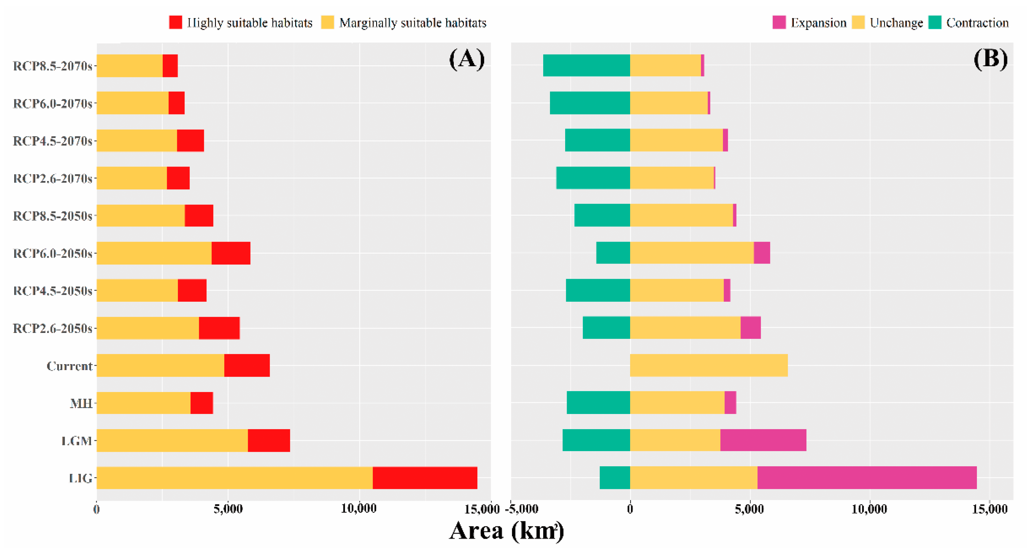
The AUC values of the models for L. oblata were higher than 0.9, indicating that our SDMs had a good performance (Table S5). Using eight bioclimatic variables, one UV-B radiation variable, and two topographic environmental variables, the training and testing AUC values of the current model were 0.9981 and 0.9962, respectively (Table S5). The training and testing AUC values of the MaxEnt model that used 25 soil variables were 0.9838 and 0.9654, respectively (Table S5). Thus, the model results can be considered satisfactory for predicting the potential suitable habitats for L. oblata. The CHS model showed that the current suitable habitats of L. oblata were primarily located in two regions: northern China, which mainly include Shanxi, Hebei, Beijing, Inner Mongolia, and Liaoning; and southwestern China, which mainly include Sichuan and Gansu. The most suitable areas were concentrated in the northern Taihang Mountains and the southern Yan Mountains (Figure 3A). According to the area calculation results, the marginally suitable and highly suitable areas of L. oblata in China were 4860.18 km2 and 1725.85 km2, respectively, and accounting for 6586.03 km2 (Figure 4A and Table S6). Notably, the current potential distribution is slightly larger than the actual distribution of L. oblata (Figure 3A).

3.2. Dynamics of Suitable Habitat Distribution under Past and Future Scenarios

Under the three paleoclimate periods, our result of the LIG indicated that the suitable habitats of L. oblata were mainly located from southwest to northeast China that including Sichuan, Gansu, Shaanxi, Henan, Shanxi, Hebei, Beijing, and Liaoning (Figure 3D); the area of suitable habitats (10,483.32 km2 and 3974.39 km2 of the marginally suitable and highly suitable areas, respectively, accounting for 14,457.71 km2) was greater than the area of suitable habitats of the current distribution (Figure 4A and Table S6). The original suitable habitat area of Sichuan and Gansu decreased significantly, and the suitable habitats in Shaanxi and Henan have been completely lost in modern times (Figure S1A,D). In total, there was 9147.47 km2 (63.27%) area expansion in the LIG than there is now (Figure 4B and Table S7). Compared with the LIG, the suitable habitats during the LGM changed slightly in location (Figure 3B,D and Figure S1B,D), but reduced by half in area which was 7360.65 km2 (5747.76 km2 and 1612.89 km2 of the marginally suitable and highly suitable areas, respectively), which was similar to the area of suitable habitats predicted by the current climate scenario (Figure 4A and Table S6). Furthermore, the suitable habitats in the MH showed a significant change in location and a great reduction in size compared with LIG, resulting in a predicted location more similar to the current climate scenario (Figure 3A,B,D). The marginally suitable and highly suitable areas in the MH were 3560.19 km2 and 859.79 km2, respectively, accounting for 4419.98 km2 (Figure 4A and Table S6).
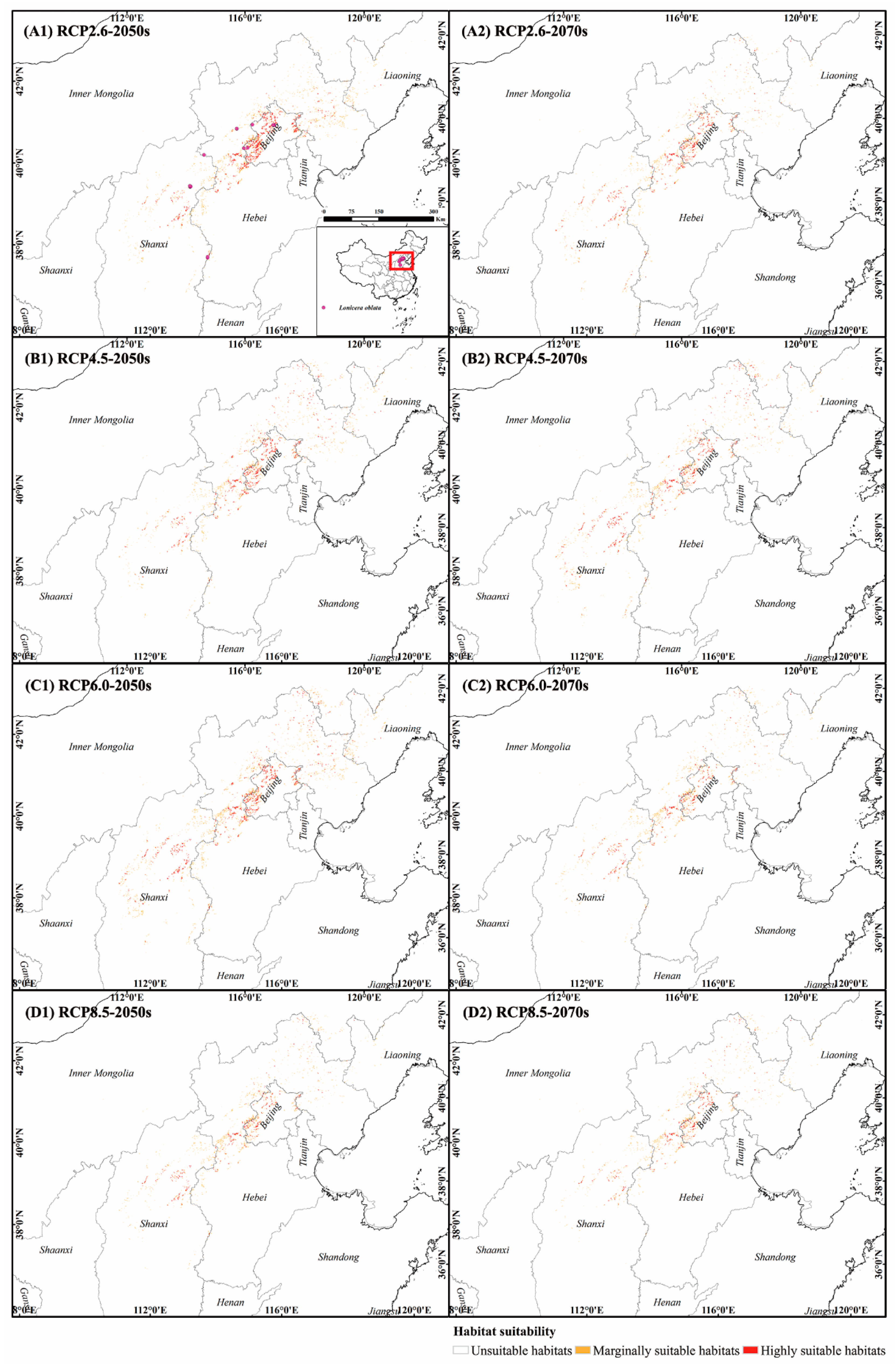
Of future global warming scenarios, our model prediction results indicated that the potential distribution area of L. oblata would decrease in eight different climate scenarios. Under four low levels of greenhouse gas emission scenarios, the suitable habitats were predicted to increase by 840.96 km2 (15.44%) by RCP2.6-2050s, mainly in northeastern Hebei, Beijing, and southwestern Liaoning, but to lose suitable habitats by 1981.37 km2 (36.38%), mainly in northeastern Sichuan, southeastern Gansu, Shanxi, and Hebei (Figure 4B and Figure S2(A1) and Table S7). By RCP2.6-2070s, the range of suitable habitats would only increase by 47.52 km2 (1.34%), mostly in scattered locations in northeastern Hebei and southwestern Beijing, but that 3085.91 km2 (86.99%) of suitable habitats would be lost (Figure 4B, Figure S2(A2) and Table S7). Compared with the RCP2.6 climate scenarios, the suitable habitat area of Beijing would be lost under RCP4.5 climate scenarios; expansions of only 275.24 km2 (6.60%) and 211.59 km2 (5.18%) were predicted in northeastern Hebei and southwestern Liaoning compared with modern times by the 2050s and 2070s, respectively (Figure 4B, Figure S2(B1,B2) and Table S7). Under high levels of greenhouse gas emission scenarios of RCP6.0 and RCP8.5, there were no significant changes in suitable habitats of L. oblata compared with that of RCP2.6 and RCP4.5 by the 2050s (Figure 4 and Figure 5 and Tables S6 and S7). However, the suitable habitats decreased dramatically to 3345.91 km2 and 3623.84 km2 under RCP6.0-2070s and RCP8.5-2070s, respectively (Figure 4B and Table S7). Overall, by comparing the eight future periods to the present time, the area of suitable habitats for L. oblata was ecologically stable from the northern Taihang Mountains to the southern Yan Mountains in Beijing.

3.3. Shifts of the Core Suitable Habitat Distributions under Climate Change Scenarios

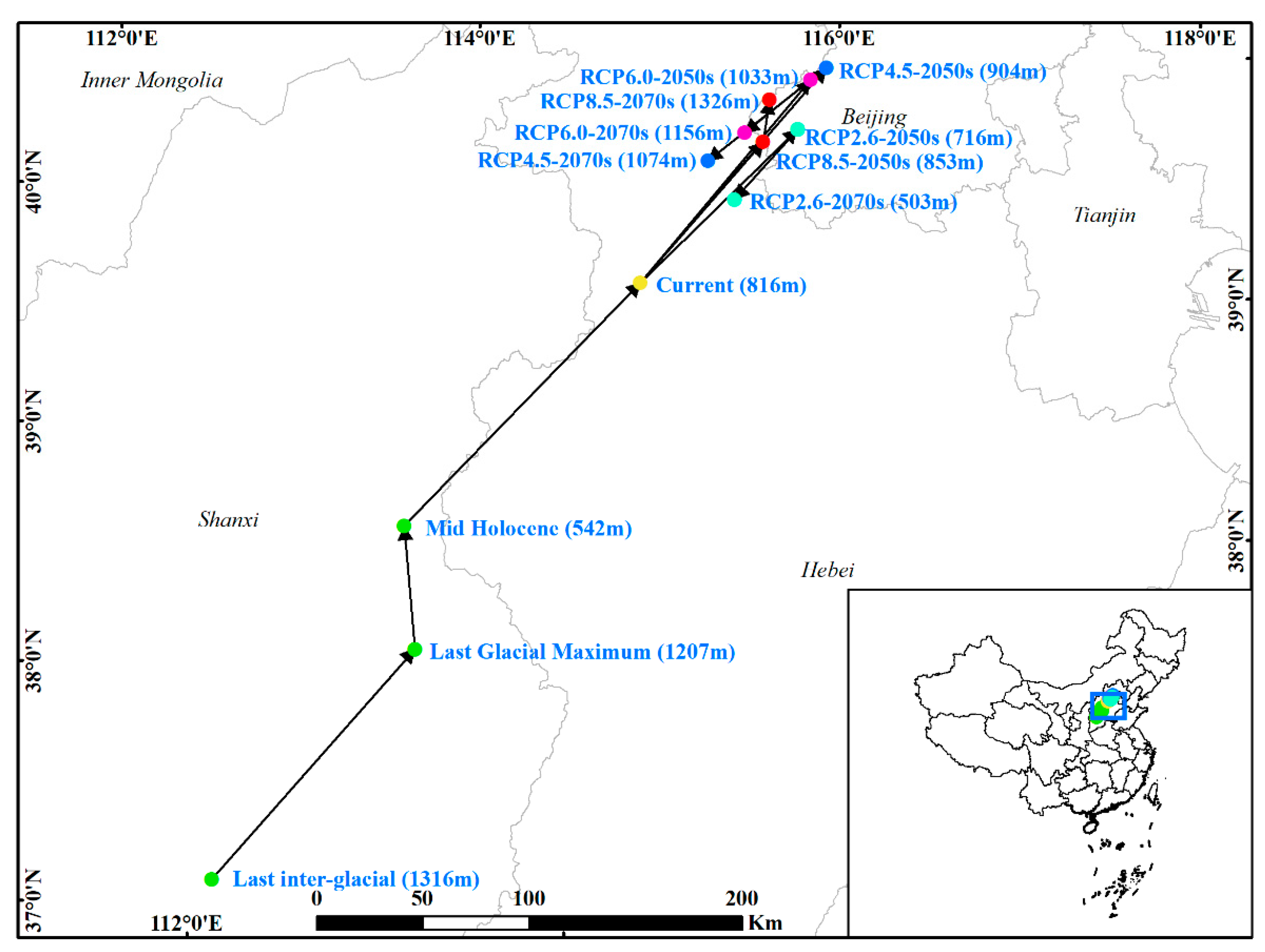
The current habitat centroid position of L. oblata represented by the yellow dot was estimated to be in central Hebei (39.3661° N, 114.7490° E). During the three paleoclimate periods (green dots), the habitat centroid of the LIG was in southwestern Shanxi (37.0331° N, 112.1550° E) and then shifted northeastward to 37.9262° N, 113.3410° E during the LGM and to 38.4423° N, 113.3400° E during the MH. Under the low-concentration greenhouse gas emission scenarios, the centroid was predicted to migrated to Beijing (39.9368° N, 115.7030° E) under RCP2.6-2050s and finally shifted to North Hebei in 2070s (39.6731° N, 115.3150° E) (cyan dots); it migrated from Beijing (40.1804° N, 115.8990° E) under RCP4.5-2050s to North Hebei in 2070s (39.8459° N, 115.1910° E) (blue dots). Under the high-concentration greenhouse gas emission scenarios, the centroid shifted to the border of Hebei and Beijing (40.1385° N, 115.8050° E) under RCP6.0-2050s, then shifted to North Hebei (39.9479° N, 115.4080° E) in 2070s (purple dots); it migrated from Beijing (39.9010° N, 115.5060° E) under RCP8.5-2050s to the border of Hebei and Beijing (40.0731° N, 115.5660° E) in 2070s (red dots). Generally, the centroid of suitable habitats for L. oblata moved toward the northeast from southwest Shanxi to the border of Hebei and southwest Beijing from the past to the future period; however, there was no significant correlation of the centroid shift observed between the low and high concentrations of greenhouse gas emissions (Figure 6 and Table S8).

3.4. Contribution of Environmental Variables to Species Distributions

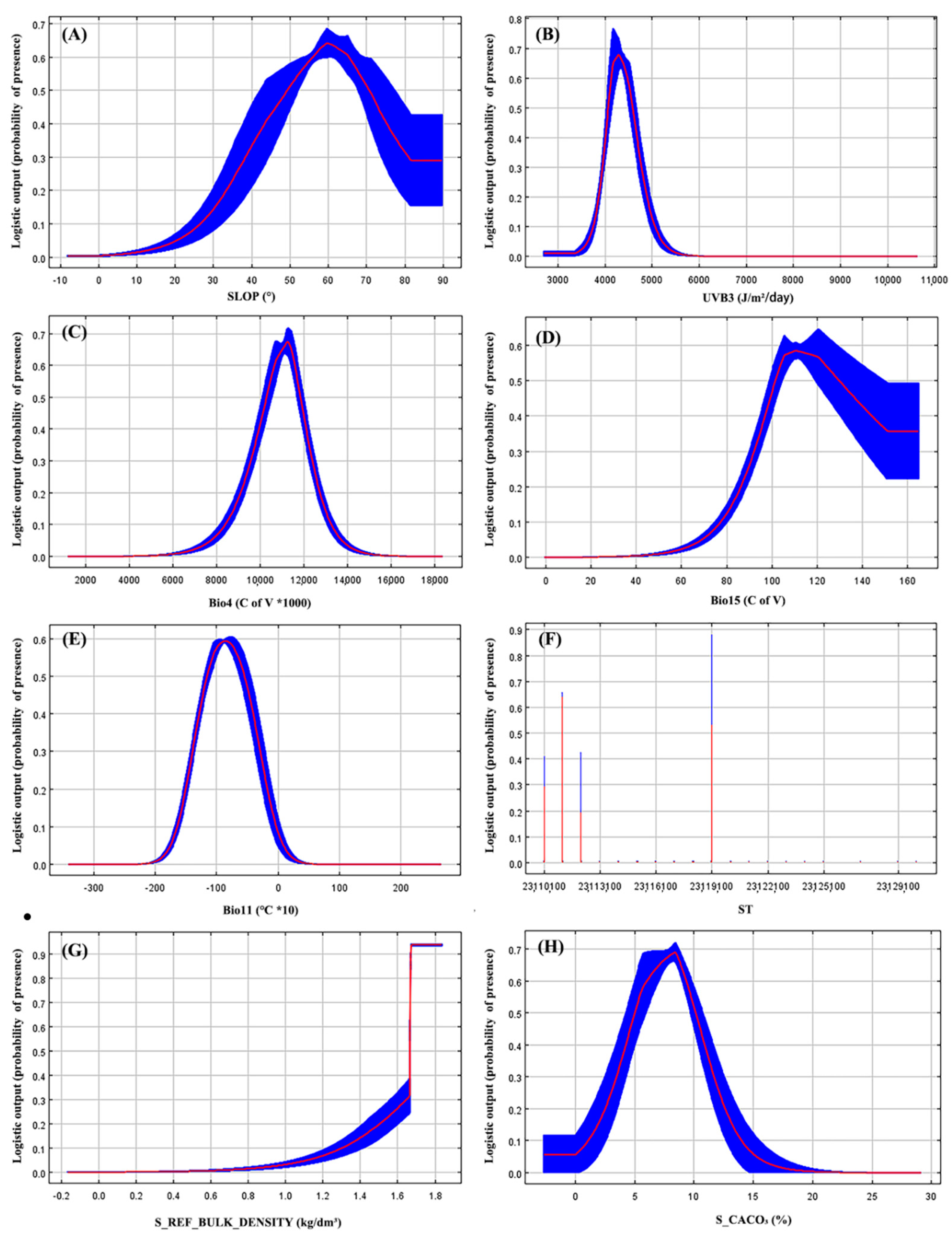
The CT MaxEnt model’s internal jackknife training of factor importance showed that slope (SLOP, 36.53 ± 0.94% of variation), mean UV-B of highest month (UVB3, 16.65 ± 1.29% of variation), temperature seasonality (Bio4, 15.37 ± 1.64% of variation), precipitation seasonality (Bio15, 11.05 ± 1.96% of variation), and mean temperature of coldest quarter (Bio11, 7.55 ± 1.42% of variation) contributed the most to the model performance for L. oblata (Table S9). The cumulative contributions of these factors reached values as high as 87.15%. To further elucidate the features of climate and geography that influenced the suitable habitats of L. oblata, we created different MaxEnt models only using one of the corresponding variables mentioned above. When the logistic probability of presence was maximal, the value of the environmental factors was optimal; when the logistic probabilities of presence were >0.3, the range of the environmental factors was within the variable threshold. Our results showed that the suitable range of slope (SLOP) ranged from 31.78° to 89.72°, and the optimal value was approximately 65.06° (Figure 7A and Table 1 and Table S10). The optimal value of UV-B of highest month (UVB3) was 4170.53 J/m2/day and ranged from 3900.26 to 4901.84 J/m2/day (Figure 7B and Table 1 and Table S10). In addition, the suitable range and optimal value of temperature seasonality (Bio4) were 9318.22 to 12,583.18 (9.32 to 12.58) and 10,693.94 (10.69), respectively (Figure 7C and Table 1 and Table S10), and the suitable range and optimal value of precipitation seasonality (Bio15) were 87.63 to 164.80 and 120.42, respectively (Figure 7D and Table 1 and Table S10). The optimal value of mean temperature of coldest quarter (Bio11) was −104.79 (−10.48 °C), ranging from −143.65 to −18.57 (−14.37 °C to −1.86 °C) (Figure 7E and Table 1 and Table S10).
Regarding the soil suitability requirements, the MaxEnt result showed that soil type variable (ST, 73.6% of variation), subsoil reference bulk density (S_REF_BULK_DENSITY, 9.6% of variation), and subsoil calcium carbonate (S_CACO3, 6.1% of variation), accounting for 89.3% of variation, were the key soil factors determining the distribution of L. oblata (Table 1 and Table S10). According to the response curves of the soil model, the optimal soil type of L. oblata was anthropogenic alluvial soil; other suitable soil types, including eluvial brown soil, semi-eluvial cinnamon soil and semi-eluvial gray cinnamon soil, were also suitable (Figure 7F and Table 1 and Table S10). The suitable range of subsoil reference bulk density (S_REF_BULK_DENSITY) ranged approximately from 1.44 to 1.84 kg/dm3, and the optimal value was approximately 1.84 kg/dm3 (Figure 7G and Table 1 and Table S10). The optimal value of subsoil calcium carbonate (S_CACO3) was 5.75%, and the threshold value of S_CACO3 ranged from 0.91% to 14.20% (Figure 7H and Table 1 and Table S10).

4. Discussion

4.1. Key Environmental Factors Shaping Species Distribution

The distributional pattern of species is the result of multiple factors, such as climate, topography, soil, human activities, species interactions, and the physiological characteristics of species [70]. In this study, we comprehensively considered the bioclimatic, UV-B, topographical, soil, vegetation, and land-use factors to simulate the potential distribution for L. oblata. The result indicated that the key factors determining the distribution of L. oblata were slope (SLOP), mean UV-B of highest month (UVB3), temperature seasonality (Bio4), precipitation seasonality (Bio15), and mean temperature of coldest quarter (Bio11). The most important soil-related variables were soil type variables (ST), subsoil reference bulk density (S_REF_BULK_DENSITY), and subsoil calcium carbonate (S_CACO3). This finding is consistent with the results of our field surveys. Specifically, populations of L. oblata were mostly observed to grow near or on the top of mountains along the Taihang and Yan mountains with the exposed limestone environments that lacking in water, poor in organic matter, low density in canopy, and with alkaline soil conditions, suggesting that slope, mean UV-B of highest month, soil type variables, subsoil reference bulk density, and subsoil calcium carbonate mainly limit the distribution of L. oblata.
Topography, including altitude, slope, aspect, and ground surface texture, is an important driver of plant species distributions through its effect on the redistribution of moisture and heat in the natural environment, especially for montane plants [64,71]. The response curve of slope (SLOP) showed that the suitable slope of L. oblata was generally greater than 31.78°. When the slope was approximately 65.06°, the logistic probability of presence reached its maximum (Table 1 and Table S10). However, the contribution value of aspect (ASPE) was 3.52 ± 0.62%, which covered a wide range from 0.15° to 309.37° (Table S10). The model estimation was highly consistent with our field observations for L. oblata, which grows on steep slopes from 30° to 75° without slope exposure limitation.
Ultraviolet (UV) radiation (280–315 nm) is an abiotic environmental factor that has significant effects on the subaerial organs of plants and limits the distribution of species, especially alpine plants, which experience some of the highest levels of UV-B irradiance [72,73]. Because the upper limits of each population of L. oblata are located near or on top of mountains with low density canopy and is consistently exposed to solar radiation, it was no surprise that one of the UV-B factors, mean UV-B of highest month (UVB3, 16.65 ± 1.29% of variation) (Table S9), was one of the most important factors in the model. L. oblata may have a limited tolerance of ultraviolet light. Prolonged exposure to intense solar UV radiation may have several potentially deleterious effects on plants, such as disrupting DNA and proteins, inducing oxidative damage, decreasing photosynthesis, inhibiting growth, and reducing the quality and yield of seeds [74,75,76,77,78]. Hence, when ultraviolet light is strong, the growth and development of L. oblata may be inhibited. Quantitative studies of the effects of UV-B radiation on the physiology of L. oblata should be performed in the future work.
Temperature and precipitation are two major environmental factors affecting the distribution of sessile plant species, especially cold tolerance, growth-season temperatures, and the available water supply for alpine vegetation [79,80]. Temperature seasonality (Bio4), precipitation seasonality (Bio15), and mean temperature of coldest quarter (Bio11) in our model each contributed greatly to the predicted distribution of L. oblata (Table 1 and Table S10), probably because the temperature during the summer is often high in China; however, the minimum temperature and temperature variation in the winter can vary substantially with latitude [81,82]. Temperature seasonality is positively correlated with latitude [83], and strong seasonal variation in temperature may inhibit the growth of vegetation [84]. Our result indicated that the suitable range of temperature seasonality (Bio4) for L. oblata was from 9.32 to 12.58 (Figure 7E and Table 1 and Table S10). Thus, temperature seasonality (Bio4) may limit the latitudinal range of L. oblata, and mean temperature of coldest quarter (Bio11) may determine whether temperatures are appropriate for vernalization. Generally, higher variation in seasonal precipitation may facilitate the presence of L. oblata.
Soil provides the necessary space and nutrients for plants to survive and also restricts their distributions [63]. In this study, we used soil variables as limiting factors to further assess the comprehensive suitability distribution of L. oblata. Our soil model results indicated that anthropogenic alluvial soil is the optimal soil type for the growth of L. oblata, followed by eluvial brown soil, semi-eluvial cinnamon soil, and semi-eluvial gray cinnamon soil. The optimal values for subsoil reference bulk density (S_REF_BULK_DENSITY), subsoil calcium carbonate (S_CACO3), subsoil CEC (soil) (S_CEC_SOIL) and topsoil gravel content (T_GRAVEL) were 1.84 kg/dm3, 5.75%, 16.54 cmol/kg, and 5%, respectively (Table S10). These characteristics conform to the unique natural habitats that L. oblata prefers to limestone soil with good cation exchange capacity. Other parameters such as topsoil organic carbon (T_OC) and topsoil pH (H2O) (T_PH) were also taken into account in our study, but they were not significant. The suitable ranges of topsoil organic carbon (T_OC) and topsoil pH (H2O) (T_PH) for L. oblata growth were 0.03%–0.88% and 6.37%–9.79%, respectively (Table S10). These results suggested the suitable soil characteristics of L. oblata habitats were characterized by alkalinity, brown calcareous soil, and a lack of organic matter.

4.2. Impacts of Climate Change on Species Range Dynamics and Migration Trends

Climate change is the main factor affecting the large-scale distribution pattern of species, and the historical factors that contributed to the development of species current distribution are often unique [85,86]. We found that changes in the area of suitable habitats in five periods for L. oblata went through a process of expansion/expansion/retreat/retreat/retreat compared with the current period (Figure 4 and Table S6). During the LIG, L. oblata had the largest distribution area and the widest geographical distribution range from northeastern Sichuan in southwest China to southwestern Liaoning in northeast China (Figure 3D). The distribution of L. oblata decreased by about half compared with the LIG, but the area of suitable habitats predicted during the LGM was still larger than that in contemporary times (Figure 3A,C,D and Figure 4). Subsequently, in the MH, the distribution of L. oblata was similar to that of the present, but area of the suitable habitats was relatively smaller (Figure 3A,B and Figure 4). This may be caused by the fact that the average annual temperature in the MH was slightly higher than that during modern times [87]. The expansion of the potential distribution area in the LIG and LGM in southwest and central China, such as in southeastern Gansu, the Qinling Mountains of Shaanxi, northwestern Henan, and southern Shanxi, was mostly lost in the MH (Figure 3). If the climate continues to warm, the potential distribution area of L. oblata is predicted to reduce to varying degrees (Figure 4, Figure 5 and Figure S2), indicating that this species is vulnerable to climate warming.
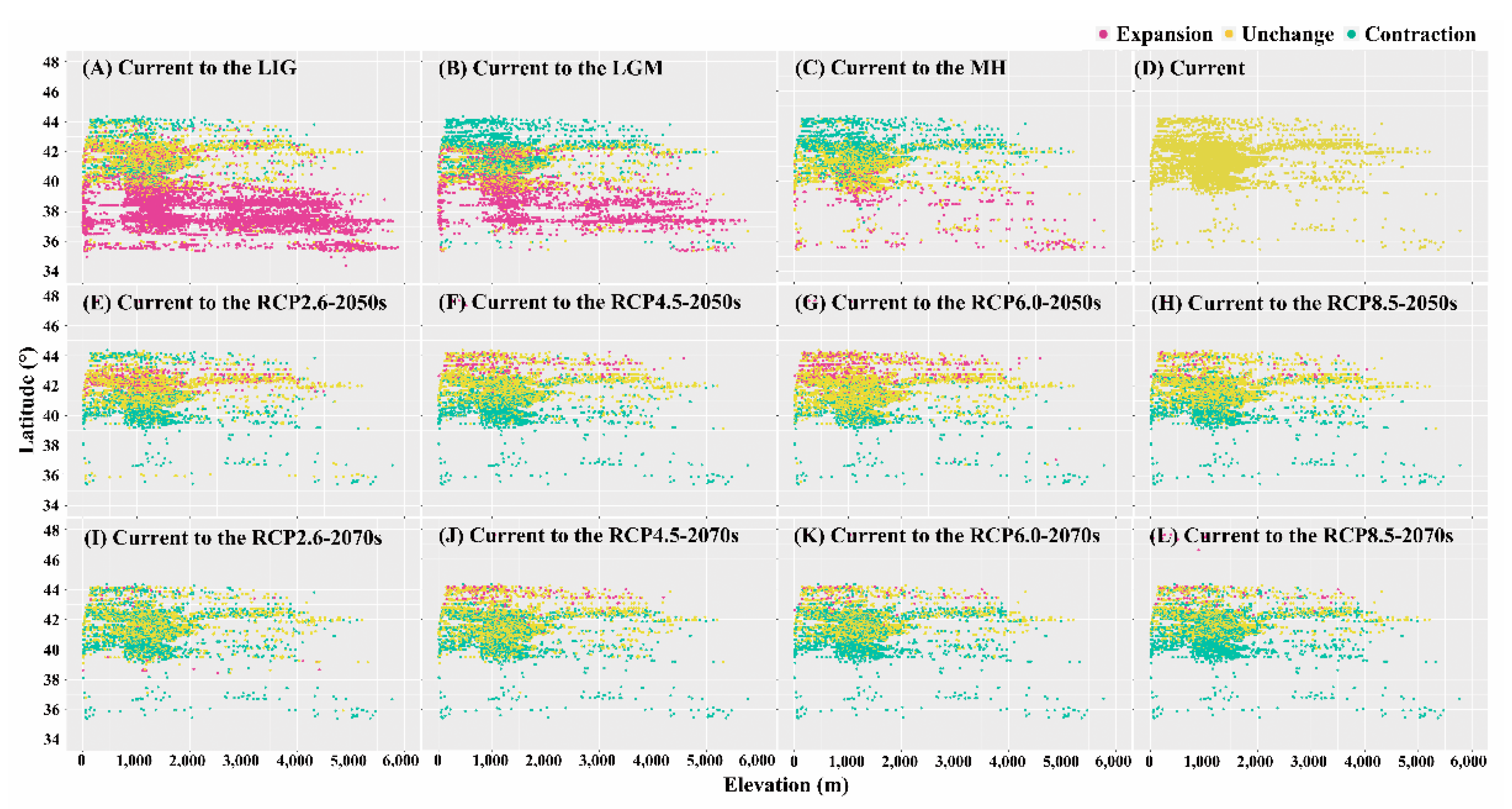
The LIG and the LGM represented contrasting extremes of climate, and L. oblata exhibited an expansion–expansion response during the late Quaternary. This pattern differs from the expansion–contraction model of temperate species distributed in Europe and North America [26,88] or contraction–expansion for cold-adapted species [10,89] in response to glacial cycles. Because of the interactions and effects of multiple factors, the historical patterns of species distribution and migration become more complicated among species [26,70]. Complex topography and greater microclimatic variation also affected historical distribution of certain species [90]. L. oblata grows on steep slopes near the tops of mountains, which are characterized unique habitat. This expansion-expansion pattern during past climatic oscillations is similar to that previously reported for the cliff plant Thuja sutchuenensis [49]. According to the paleodistribution models, the area of suitable habitats for L. oblata at lower latitudes decreased from the past to the present, and the centroid moved northward (Figure 6 and Figure 8).
In response to global warming, some species may remain in place via physiological or phenological adaptation [91,92], but several species will migrate to higher latitudes or higher elevations to escape warming temperatures [7]. Our findings suggested that the suitable habitats of L. oblata drastically contracted at lower latitudes and slightly expanded at higher latitudes with future climate warming, but there was no obvious altitudinal migration (Figure 8). This result further suggested that L. oblata would have a more limited geographic range under future climate warming (Figure 4, Figure 5, Figure 8 and Figure S2). This finding implies that, for higher elevation montane species such as L. oblata, there may be insufficient suitable alpine habitat to facilitate future migration. Thus, for this species at least, prediction of future distribution is consistent with the “nowhere to go” hypothesis.

4.3. Stable Climatic Areas, Risks to Species in Climate-Vulnerable Areas, and Conservation Management

We identified the stable climatic areas of L. oblata that likely to have been or will be suitable from the LIG to current and until at least 2070s. Paleoclimate change may have profoundly influenced the historical space and population dynamics of ancient L. oblata. Our results suggest that the border of Sichuan and Gansu, the southern border of Shaanxi and Gansu, and the southern Lüliang Mountains and Taihang Mountains may have provided important stable climatic areas (Figure S3). Comparison of the changes under the current and eight future scenarios revealed that the central and northern regions of the Taihang Mountains, the north part of the Lüliang Mountains and Yan Mountains were stable areas with suitable habitats that could facilitate the presence of L. oblata in response to future climate change (Figure S3). These regions may provide future stable climatic areas for L. oblata and be vital for future conservation efforts.
Distribution models predicted severe range contractions of suitable habitats in the future for both high and low emission scenarios (Figure 4 and Figure S2 and Table S7), indicating L. oblata is susceptible to climate change. Nearly half of the potential distributions, particularly in southern Shanxi, the border of Shanxi and Hebei, and northeastern Hebei were identified as climate-vulnerable areas for L. oblata (Figure S2). It grows near or on the top of the mountains with calcium carbonate soil; there is an insufficient amount of suitable habitats at higher altitudes for migration to permit escape from global warming through changes in elevation [10,30,31,32]. Furthermore, other species from lower elevations may migrate upward to exert pressure on the original habitats of L. oblata [93,94]. This spatial limitation restriction and interspecific competition might cause a rapid loss of suitable habitats [31,34,95] as L. oblata approaches mountain peaks. Additionally, there was a low occurrence of new suitable areas in response to different climate change scenarios (Figure 4 and Figure S2 and Table S7). Normally, the habitats of plants growing on the tops of the mountains are surrounded by forests, making them into isolated and fragmented islands that increase the difficulty of the migration of pollen and fruit and prevent long-distance dispersal [49,60]. Hence, biogeographic barriers such as mountain ranges may limit the migration of L. oblata [34]. Hence, future climate warming may drive L. oblata into a “nowhere-to-go” scenario and this endangered montane shrub are facing a high risk of extinction. There is thus an urgent need to develop effective conservation strategies and long-term conservation actions for L. oblata.
Our field surveys showed that L. oblata only grows near or on the top of the Taihang and Yan mountains; most L. oblata populations were scattered in isolated patches of habitats, this was a challenge to collect existing locations and discover new populations of L. oblata. Several studies have successfully used species distribution model to predict species distribution and to detect previously unknown populations of endangered species [46,49]. In this study, we predicted new areas with suitable habitats for L. oblata; new areas were primarily located in the north of the Lüliang Mountains, the north of the Yan Mountains, and the border of Gansu–Sichuan (Figure 3A). So far, no record of L. oblata has been obtained from these newly identified suitable habitats; and further field surveys should be conducted. Additionally, in situ conservation strategies, such as the establishment of nature reserves, should be implemented. During our field studies, L. oblata was observed to suffer from the effects of logging, mining, overgrazing, and tourism. Hence, ex situ should also be planned for certain populations. Future conservation efforts should also involve the establishment of botanical gardens and core germplasm via the transplantation and cultivation of seedlings.

4.4. Model Rationality and Drawback

Environmental variables including topography, soil, vegetation, and land-use were set invariable in all six periods because of the lack of these data so far. These variables might not stay the same over time for a long period from the LIG to 2070s. It is also hard to model some ecological and evolutionary processes which may greatly affect the distribution of species, such as species interactions and human activities. However, our field investigation shows that L. oblata growing in the limestone cliff-habitat in shrubland and alpine meadows with low density in canopy. For unique growth requirements of L. oblata, the suitable vegetation and soil conditions are of great importance on the distribution of this species, even though climate is favorable. To make the prediction results more realistic, we further built a CHS model following previous studies [61,62,63,64] to assess the distribution of suitable habitats of L. oblata using the soil, vegetation, and land-use conditions as overlying variables. The AUC values of the models for L. oblata were higher than 0.9, indicating that our SDMs had an excellent performance (Table S5). Our results also showed the current potential distribution is highly consistent with our field research. Hence, the model results can be considered adequacy for predicting the potential suitable habitats for L. oblata, and SDMs and CHS model can provide valuable information for the practical conservation of endangered species.

5. Conclusions

In this study, we built the CHS model that considered bioclimatic, UVB radiation, topographical, edaphic, vegetation, and land-use demands to simulate the distribution pattern and dynamic of L. oblata in response to climate change since the LIG. The predicted current potential distribution of L. oblata was primarily located in North China (Beijing, Hebei, Shanxi, Inner Mongolia, and Liaoning), and it was most influenced by SLOP, UVB3, Bio4, Bio15, Bio11, ST, S_REF_BULK_DENSITY, and S_CACO3. Historically, L. oblata underwent a significant range expansion during the LIG and the LGM, but a slight range contraction during the MH. Under various future climate scenarios, the potential suitable areas of L. oblata were predicted to shrink at varied degrees latitudinal while no strong altitudinal relevance was detected. Consequently, this species is likely to face a “nowhere to go” predicament. Our work provides an important reference for the conservation of L. oblata and other endangered montane species under climate change.

Supplementary Materials

The following are available online at https://www.mdpi.com/1999-4907/12/2/125/s1, Figure S1: Suitable habitat changes under the past periods compared with the current condition; Figure S2: Suitable habitat changes under eight future periods compared with the current condition; Figure S3: The stable climatic areas of paleoclimate and future climate; Table S1: 23 species presence data for MaxEnt modeling; Table S2: Information of 65 environmental variables; Table S3 Correlations among 28 climatic variables; Table S4: Correlations among 35 soil variables; Table S5: The mean area under the curve (AUC) from 10 replicate models of Lonicera oblata under three past, present and eight future climate scenarios and soil model; Table S6: Two suitability levels of distribution areas of Lonicera oblata under three past, present and eight future climate scenarios; Table S7: Suitable habitats migration of Lonicera oblata under three past and eight future climate scenarios compared to the current; Table S8: Geographic coordinates and elevation of suitable area centroids of Lonicera oblata under twelve scenarios; Table S9: The contribution values for 11 environmental variables of CT model under twelve scenarios; Table S10: Contribution value, optimal and threshold values for each selected environmental variable under current scenario.

Author Contributions

Conceptualization, X.-Y.M.; methodology, X.-Y.M. and Y.-M.W.; software, Y.-M.W. and L.T.; validation, Y.-M.W., X.-L.S., L.T., F.-W.L., X.-Y.M., and Z.-X.Z.; formal analysis, Y.-M.W. and X.-L.S.; investigation, Y.-M.W., X.-L.S., L.T., and F.-W.L.; resources, X.-Y.M. and Z.-X.Z.; data curation, Y.-M.W.; writing—original draft preparation, Y.-M.W.; X.-L.S., L.T., and F.-W.L. writing—review and editing, X.-Y.M.; visualization, Y.-M.W.; supervision, X.-Y.M. and Z.-X.Z.; project administration, X.-Y.M.; funding acquisition, X.-Y.M. All authors have read and agreed to the published version of the manuscript.

Funding

This research was funded by the Beijing Natural Science Foundation (No.5192012) and the Natural Science Foundation of China (No. 32070235).

Acknowledgments

We would like to thank the contributors to the databases used in this study. We also appreciate the help from Nan Yang for field investigation at Dongling Mountain, Beijing, Ying-Chun Xie for field investigation at Bijia Mountain, Hebei Province, and Jian He for data analysis.

Conflicts of Interest

The authors declare no conflict of interest.

References

  1. Novacek, M.J. The Biodiversity Crisis: Losing What Counts; The New Press: New York, NY, USA, 2001. [Google Scholar]
  2. Raup, D.M.; Sepkoski, J.J. Mass extinctions in the marine fossil record. Science 1982, 215, 1501–1503. [Google Scholar] [CrossRef] [PubMed] [Green Version]
  3. Jablonski, D. Extinctions in the fossil record. Philos. Trans. R. Soc. B Biol. Sci. 1994, 344, 11–17. [Google Scholar] [CrossRef]
  4. Bambach, R.K. Phanerozoic biodiversity mass extinctions. Annu. Rev. Earth Planet. Sci. 2006, 34, 127–155. [Google Scholar] [CrossRef]
  5. Barnosky, A.D.; Matzke, N.; Tomiya, S.; Wogan, G.O.U.; Swartz, B.; Quental, T.B.; Marshall, C.R.; McGuire, J.L.; Lindsey, E.L.; Maguire, K.C.; et al. Has the Earth’s sixth mass extinction already arrived? Nature 2011, 471, 51–57. [Google Scholar] [CrossRef]
  6. Novacek, M.J.; Cleland, E.E. The current biodiversity extinction event: Scenarios for mitigation and recovery. Proc. Natl. Acad. Sci. USA 2001, 98, 5466–5470. [Google Scholar] [CrossRef] [PubMed] [Green Version]
  7. Root, T.L.; Price, J.T.; Hall, K.R.; Schneider, S.H.; Rosenzweigk, C.; Pounds, J.A. Fingerprints of global warming on wild animals and plants. Nature 2003, 421, 57–60. [Google Scholar] [CrossRef]
  8. Chen, I.-C.; Hill, J.K.; Ohlemüller, R.; Roy, D.B.; Thomas, C.D. Rapid range shifts of species associated with high levels of climate warming. Science 2011, 333, 1024–1026. [Google Scholar] [CrossRef]
  9. IPCC. Climate Change 2013: The Physical Science Basis. Contribution of Working Group I to the Fifth Assessment Report of the Intergovernmental Panel on Climate Change; Stocker, T.F., Qin, D., Plattner, G.-K., Tignor, M., Allen, S.K., Boschung, J., Nauels, A., Xia, Y., Bex, V., Midgley, P.M., Eds.; Cambridge University Press: New York, NY, USA, 2013; Volume 1535. [Google Scholar]
  10. You, J.; Qin, X.; Ranjitkar, S.; Lougheed, S.C.; Wang, M.; Zhou, W.; Ouyang, D.; Zhou, Y.; Xu, J.; Zhang, W.; et al. Response to climate change of montane herbaceous plants in the genus Rhodiola predicted by ecological niche modelling. Sci. Rep. 2018, 8, 5879. [Google Scholar] [CrossRef]
  11. Bai, Y.; Wei, X.; Li, X. Distributional dynamics of a vulnerable species in response to past and future climate change: A window for conservation prospects. PeerJ 2018, 6, e4287. [Google Scholar] [CrossRef]
  12. Araújo, M.B.; Rahbek, C. How does climate change affect biodiversity? Science 2006, 313, 1396–1397. [Google Scholar] [CrossRef] [PubMed]
  13. Beaumont, L.J.; Pitman, A.J.; Poulsen, M.; Hughes, L. Where will species go? Incorporating new advances in climate modelling into projections of species distributions. Glob. Chang. Biol. 2007, 13, 1368–1385. [Google Scholar] [CrossRef]
  14. Lenoir, J.; Gégout, J.-C.; Marquet, P.A.; De Ruffray, P.; Brisse, H. A Significant upward shift in plant species optimum elevation during the 20th century. Science 2008, 320, 1768–1771. [Google Scholar] [CrossRef] [PubMed]
  15. Comes, H.P.; Kadereit, J.W. The effect of Quaternary climatic changes on plant distribution and evolution. Trends Plant Sci. 1998, 3, 432–438. [Google Scholar] [CrossRef]
  16. Hewitt, G.M. The genetic legacy of the quaternary ice ages. Nature 2000, 405, 907–913. [Google Scholar] [CrossRef] [PubMed]
  17. Sandel, B.; Arge, L.; Dalsgaard, B.; Davies, R.G.; Gaston, K.J.; Sutherland, W.J.; Svenning, J.-C. The influence of late quaternary climate-change velocity on species endemism. Science 2011, 334, 660–664. [Google Scholar] [CrossRef] [Green Version]
  18. Dawson, A.G. Ice Age Earth: Late Quaternary Geology and Climate; Routledge: New York, NY, USA, 1992. [Google Scholar]
  19. Fačkovcová, Z.; Senko, D.; Svitok, M.; Guttová, A. Ecological niche conservatism shapes the distributions of lichens: Geographical segregation does not reflect ecological differentiation. Preslia 2017, 89, 63–85. [Google Scholar] [CrossRef]
  20. Clark, P.U.; Dyke, A.S.; Shakun, J.D.; Carlson, A.E.; Clark, J.; Wohlfarth, B.; Mitrovica, J.X.; Hostetler, S.W.; McCabe, A.M. The last glacial maximum. Science 2009, 325, 710–714. [Google Scholar] [CrossRef] [Green Version]
  21. Nogués-Bravo, D.; Ohlemüller, R.; Batra, P.; Araújo, M.B. Climate predictors of late quaternary extinctions. Evolution 2010, 64, 2442–2449. [Google Scholar] [CrossRef]
  22. Davis, M.B. Range shifts and adaptive responses to quaternary climate change. Science 2001, 292, 673–679. [Google Scholar] [CrossRef] [PubMed] [Green Version]
  23. Normand, S.; Ricklefs, R.E.; Skov, F.; Bladt, J.; Tackenberg, O.; Svenning, J.-C. Postglacial migration supplements climate in determining plant species ranges in Europe. Proc. R. Soc. B Boil. Sci. 2011, 278, 3644–3653. [Google Scholar] [CrossRef] [PubMed]
  24. Svenning, J.-C.; Skov, F. Ice age legacies in the geographical distribution of tree species richness in Europe. Glob. Ecol. Biogeogr. 2007, 16, 234–245. [Google Scholar] [CrossRef]
  25. Feng, G.; Ma, Z.; Sandel, B.; Mao, L.; Normand, S.; Ordonez, A.; Svenning, J. Species and phylogenetic endemism in angiosperm trees across the Northern Hemisphere are jointly shaped by modern climate and glacial–interglacial climate change. Glob. Ecol. Biogeogr. 2019, 28, 1393–1402. [Google Scholar] [CrossRef]
  26. Provan, J.; Bennett, K.D. Phylogeographic insights into cryptic glacial refugia. Trends Ecol. Evol. 2008, 23, 564–571. [Google Scholar] [CrossRef] [PubMed]
  27. Leadley, P.; Pereira, H.M.; Alkemade, R.; Fernandez-Manjarrés, J.F.; Proenca, V.; Scharlemann, J.P.W.; Walpole, M.J. Biodiversity Scenarios: Projections of 21st Century Change in Biodiversity and Associated Ecosystem Services; Secretariat of the Convention on Biological Diversity: Montreal, QC, Canada, 2010. [Google Scholar]
  28. Hickling, R.; Roy, D.B.; Hill, J.K.; Fox, R.; Thomas, C.D. The distributions of a wide range of taxonomic groups are expanding polewards. Glob. Chang. Biol. 2006, 12, 450–455. [Google Scholar] [CrossRef]
  29. Pecl, G.T.; Araújo, M.B.; Bell, J.D.; Blanchard, J.; Bonebrake, T.C.; Chen, I.-C.; Clark, T.D.; Colwell, R.K.; Danielsen, F.; Evengård, B.; et al. Biodiversity redistribution under climate change: Impacts on ecosystems and human well-being. Science 2017, 355, eaai9214. [Google Scholar] [CrossRef]
  30. Nogués-Bravo, D.; Araújo, M.B.; Errea, M.P.; Martínez-Rica, J.P. Exposure of global mountain systems to climate warming during the 21st century. Glob. Environ. Chang. 2007, 17, 420–428. [Google Scholar] [CrossRef]
  31. Colwell, R.K.; Brehm, G.; Cardelús, C.L.; Gilman, A.C.; Longino, J.T. Global warming, elevational range shifts, and lowland biotic attrition in the wet tropics. Science 2008, 322, 258–261. [Google Scholar] [CrossRef] [Green Version]
  32. Loarie, S.R.; Duffy, P.B.; Hamilton, H.; Asner, G.P.; Field, C.B.; Ackerly, D.D. The velocity of climate change. Nature. 2009, 462, 1052–1055. [Google Scholar] [CrossRef]
  33. Broennimann, O.; Thuiller, W.; Hughes, G.; Midgley, G.F.; Alkemade, J.M.R.; Guisan, A. Do geographic distribution, niche property and life form explain plants’ vulnerability to global change? Glob. Chang. Biol. 2006, 12, 1079–1093. [Google Scholar] [CrossRef]
  34. Boulangeat, I.; Gravel, D.; Thuiller, W. Accounting for dispersal and biotic interactions to disentangle the drivers of species distributions and their abundances. Ecol. Lett. 2012, 15, 584–593. [Google Scholar] [CrossRef]
  35. Malcolm, J.R.; Liu, C.; Neilson, R.P.; Hansen, L.; Hannah, L. Global warming and extinctions of endemic species from biodiversity hotspots. Conserv. Biol. 2006, 20, 538–548. [Google Scholar] [CrossRef] [PubMed]
  36. Guisan, A.; Zimmermann, N.E. Predictive habitat distribution models in ecology. Ecol. Model. 2000, 135, 147–186. [Google Scholar] [CrossRef]
  37. Elith, J.; Leathwick, J.R. Species distribution models: Ecological explanation and prediction across space and time. Annu. Rev. Ecol. Evol. Syst. 2009, 40, 677–697. [Google Scholar] [CrossRef]
  38. Guisan, A.; Thuiller, W. Predicting species distribution: Offering more than simple habitat models. Ecol. Lett. 2005, 8, 993–1009. [Google Scholar] [CrossRef]
  39. Kearney, M.R.; Wintle, B.A.; Porter, W.P. Correlative and mechanistic models of species distribution provide congruent forecasts under climate change. Conserv. Lett. 2010, 3, 203–213. [Google Scholar] [CrossRef]
  40. Baker, D.J.; Hartley, A.J.; Butchart, S.H.M.; Willis, S.G. Choice of baseline climate data impacts projected species’ responses to climate change. Glob. Chang. Biol. 2016, 22, 2392–2404. [Google Scholar] [CrossRef] [Green Version]
  41. Busby, J.R. BIOCLIM: A bioclimate analysis and prediction system. Plant Prot. Q. 1991, 6, 8–9. [Google Scholar]
  42. Stockwell, D. The GARP modelling system: Problems and solutions to automated spatial prediction. Int. J. Geogr. Inf. Sci. 1999, 13, 143–158. [Google Scholar] [CrossRef]
  43. Bradter, U.; Kunin, W.E.; Altringham, J.D.; Thom, T.J.; Benton, T.G. Identifying appropriate spatial scales of predictors in species distribution models with the random forest algorithm. Methods Ecol. Evol. 2013, 4, 167–174. [Google Scholar] [CrossRef]
  44. Phillips, S.J.; Dudík, M.; Schapire, R.E. A maximum entropy approach to species distribution modeling. In Proceedings of the Twenty-First International Conference on Machine Learning—ICML ’04, Banff, AB, Canada, 4–8 July 2004; Volume 9, pp. 655–662. [Google Scholar]
  45. Elith, J.; Graham, C.H.; Anderson, R.P.; Dudík, M.; Ferrier, S.; Guisan, A.; Hijmans, R.J.; Huettmann, F.; Leathwick, J.R.; Lehmann, A.; et al. Novel methods improve prediction of species’ distributions from occurrence data. Ecography 2006, 29, 129–151. [Google Scholar] [CrossRef] [Green Version]
  46. Phillips, S.J.; Anderson, R.P.; Schapire, R.E. Maximum entropy modeling of species geographic distributions. Ecol. Model. 2006, 190, 231–259. [Google Scholar] [CrossRef] [Green Version]
  47. Pearson, R.G.; Raxworthy, C.J.; Nakamura, M.; Townsend Peterson, A. Predicting species distributions from small numbers of occurrence records: A test case using cryptic geckos in Madagascar. J. Biogeogr. 2007, 34, 102–117. [Google Scholar] [CrossRef]
  48. Rebelo, H.; Jones, G. Ground validation of presence-only modelling with rare species: A case study on barbastelles Barbastella barbastellus (Chiroptera: Vespertilionidae). J. Appl. Ecol. 2010, 47, 410–420. [Google Scholar] [CrossRef]
  49. Qin, A.; Liu, B.; Guo, Q.; Bussmann, R.W.; Ma, F.; Jian, Z.; Xu, G.; Pei, S. Maxent modeling for predicting impacts of climate change on the potential distribution of Thuja sutchuenensis Franch., an extremely endangered conifer from southwestern China. Glob. Ecol. Conserv. 2017, 10, 139–146. [Google Scholar] [CrossRef]
  50. Wu, Z.Y.; Raven, P.H.; Hong, D.Y. Caprifoliaceae. In Flora of China; Yang, Q.E., Landrein, S., Osborne, J., Eds.; Science Press: Beijing, China, 2011; Volume 19, pp. 616–641. [Google Scholar]
  51. Jiang, W.J.; Wu, J.G.; Ren, J.W.; Bin, Y.B.; Wang, T. The research of characteristics of Lonicera oblata. Chin. Hortic. Abs. 2015, 5. [Google Scholar]
  52. Liu, Q.R.; Kang, M.Y.; Jiang, Y. Some new recorded plants from Beijing and Hebei (Ⅱ). J. Beijing Norm. Univ. (Nat. Sci.) 2003, 39, 674–676. [Google Scholar]
  53. Hijmans, R.J.; Cameron, S.E.; Parra, J.L.; Jones, P.G.; Jarvis, A. Very high resolution interpolated climate surfaces for global land areas. Int. J. Clim. 2005, 25, 1965–1978. [Google Scholar] [CrossRef]
  54. Gent, P.R.; Danabasoglu, G.; Donner, L.J.; Holland, M.M.; Hunke, E.C.; Jayne, S.R.; Lawrence, D.M.; Neale, R.B.; Rasch, P.J.; Vertenstein, M.; et al. The community climate system model version 4. J. Clim. 2011, 24, 4973–4991. [Google Scholar] [CrossRef]
  55. Beckmann, M.; Václavík, T.; Manceur, A.M.; Šprtová, L.; Von Wehrden, H.; Welk, E.; Cord, A.F. glUV: A global UV-B radiation data set for macroecological studies. Methods Ecol. Evol. 2014, 5, 372–383. [Google Scholar] [CrossRef]
  56. Wu, D.; Zhao, X.; Liang, S.; Zhou, T.; Huang, K.; Tang, B.; Zhao, W. Time-lag effects of global vegetation responses to climate change. Glob. Chang. Biol. 2015, 21, 3520–3531. [Google Scholar] [CrossRef]
  57. Shabani, F.; Ahmadi, M.; Peters, K.; Haberle, S.; Champreux, A.; Saltre, F.B.; Bradshaw, C.J.A. Climate-driven shifts in the distribution of koala-browse species from the Last Interglacial to the near future. Ecography 2019, 42, 1587–1599. [Google Scholar] [CrossRef] [Green Version]
  58. Graham, M.H. Confronting multicollinearity in ecological multiple regression. Ecology 2003, 84, 2809–2815. [Google Scholar] [CrossRef] [Green Version]
  59. Breiner, F.T.; Guisan, A.; Bergamini, A.; Nobis, M.P. Overcoming limitations of modelling rare species by using ensembles of small models. Methods Ecol. Evol. 2015, 6, 1210–1218. [Google Scholar] [CrossRef]
  60. Li, M.; He, J.; Zhao, Z.; Lyu, R.; Yao, M.; Cheng, J.; Xie, L. Predictive modelling of the distribution of Clematis sect. Fruticella s. str. under climate change reveals a range expansion during the Last Glacial Maximum. PeerJ 2020, 8, e8729. [Google Scholar] [CrossRef] [PubMed] [Green Version]
  61. Guo, Y.; Li, X.; Zhao, Z.; Wei, H.; Gao, B.; Gu, W. Prediction of the potential geographic distribution of the ectomycorrhizal mushroom Tricholoma matsutake under multiple climate change scenarios. Sci. Rep. 2017, 7, srep46221. [Google Scholar] [CrossRef] [PubMed] [Green Version]
  62. Guo, Y.; Li, X.; Zhao, Z.; Nawaz, Z. Predicting the impacts of climate change, soils and vegetation types on the geographic distribution of Polyporus umbellatus in China. Sci. Total. Environ. 2019, 648, 1–11. [Google Scholar] [CrossRef]
  63. Liu, J.; Yang, Y.; Wei, H.Y.; Zhang, Q.Z.; Zhang, X.H.; Zhang, X.Y.; Gu, W. Assessing habitat suitability of parasitic plant cistanche deserticola in Northwest China under future climate scenarios. Forests 2019, 10, 823. [Google Scholar] [CrossRef] [Green Version]
  64. Zhao, Z.; Guo, Y.; Wei, H.; Ran, Q.; Liu, J.; Zhang, Q.; Gu, W. Potential distribution of Notopterygium incisum Ting ex H. T. Chang and its predicted responses to climate change based on a comprehensive habitat suitability model. Ecol. Evol. 2020, 10, 3004–3016. [Google Scholar] [CrossRef]
  65. Baldwin, R.A. Use of maximum entropy modeling in wildlife research. Entropy 2009, 11, 854–866. [Google Scholar] [CrossRef]
  66. Fielding, A.H.; Bell, J.F. A review of methods for the assessment of prediction errors in conservation presence/absence models. Environ. Conserv. 1997, 24, 38–49. [Google Scholar] [CrossRef]
  67. Wang, Y.S.; Xie, B.Y.; Wan, F.H.; Xiao, Q.M.; Dai, L.Y. Application of ROC curve analysis in evaluating the performance of alien species' potential distribution models. Biodivers. Sci. 2007, 15, 365–372. [Google Scholar] [CrossRef]
  68. Swets, J.A. Measuring the accuracy of diagnostic systems. Science 1988, 240, 1285–1293. [Google Scholar] [CrossRef] [PubMed] [Green Version]
  69. Brown, J.L. SDMtoolbox: A python-based GIS toolkit for landscape genetic, biogeographic and species distribution model analyses. Methods Ecol. Evol. 2014, 5, 694–700. [Google Scholar] [CrossRef]
  70. Chahouki, M.A.Z.; Khojasteh, F.; Tavili, A. Distribution of vegetation type according to edaphic properties and topography in Iran. Pol. J. Environ. Stud. 2012, 21, 1071–1077. [Google Scholar]
  71. Wang, J.; Wang, Y.; Feng, J.; Chen, C.; Chen, J.; Long, T.; Li, J.-Q.; Zang, R.; Li, J. Differential responses to climate and land-use changes in threatened chinese taxus species. Forests 2019, 10, 766. [Google Scholar] [CrossRef] [Green Version]
  72. Caldwell, M.M. Solar ultraviolet radiation as an ecological factor for alpine plants. Ecol. Monogr. 1968, 38, 243–268. [Google Scholar] [CrossRef]
  73. Blumthaler, M.; Ambach, W.; Ellinger, R. Increase in solar UV radiation with altitude. J. Photochem. Photobiol. B: Biol. 1997, 39, 130–134. [Google Scholar] [CrossRef]
  74. Bornman, J.F.; Teramura, A.H. Effects of Ultraviolet-B Radiation on Terrestrial Plants; Young, A.R., Björn, L.O., Moan, J., Nultsch, W., Eds.; Environmental UV Photobiology: Springer, Boston, MA, USA, 1993. [Google Scholar]
  75. Battaglia, P.R.; Brennan, T.M. Differential effects of short-term exposure to ultraviolet-b radiation upon photosynthesis in cotyledons of a resistant and a susceptible species. Int. J. Plant Sci. 2000, 161, 771–778. [Google Scholar] [CrossRef]
  76. Albert, K.R.; Mikkelsen, T.N.; Ro-Poulsen, H.; Arndal, M.F.; Michelsen, A. Ambient UV-B radiation reduces PSII performance and net photosynthesis in high Arctic Salix arctica. Environ. Exp. Bot. 2011, 73, 10–18. [Google Scholar] [CrossRef]
  77. Jansen, M.A.; Bornman, J.F. UV-B radiation: From generic stressor to specific regulator. Physiol. Plant. 2012, 145, 501–504. [Google Scholar] [CrossRef]
  78. Hideg, É.; Jansen, M.A.K.; Strid, Å. UV-B exposure, ROS, and stress: Inseparable companions or loosely linked associates? Trends Plant Sci. 2013, 18, 107–115. [Google Scholar] [CrossRef] [PubMed] [Green Version]
  79. Woodwand, F.I. Climate and Plant Distribution; Cambridge University Press: Cambridge, UK, 1987. [Google Scholar]
  80. Zhong, L.; Ma, Y.; Salama, M.S.; Su, Z. Assessment of vegetation dynamics and their response to variations in precipitation and temperature in the Tibetan Plateau. Clim. Chang. 2010, 103, 519–535. [Google Scholar] [CrossRef]
  81. Chen, M.R. A preliminary study on climate regionalization in China. Sci. Geogr. Sin. 1990, 4. [Google Scholar]
  82. Lin, L.; He, J.; Xie, L.; Cui, G. Prediction of the suitable area of the Chinese white pines (Pinus subsect. Strobus) under climate changes and implications for their conservation. Forests 2020, 11, 996. [Google Scholar] [CrossRef]
  83. Feng, J.M. Spatial patterns of species diversity of seed plants in China and their climatic explanation. Biodivers. Sci. 2008, 16, 470. [Google Scholar] [CrossRef]
  84. Yang, Q.-S.; Xing, Y.; Zhou, Z.-K. Modern geographical distribution of tsuga and its climatic conditions in the Asian monsoon region. Acta Bot. Yunnanica 2009, 31, 389–398. [Google Scholar] [CrossRef]
  85. Pearson, R.G.; Dawson, T.P. Predicting the impacts of climate change on the distribution of species: Are bioclimate envelope models useful? Glob. Ecol. Biogeogr. 2003, 12, 361–371. [Google Scholar] [CrossRef] [Green Version]
  86. Loidi, J.; Biurrun, I.; Campos, J.A.; García-Mijangos, I.; Herrera, M. A biogeographical analysis of the European Atlantic lowland heathlands. J. Veg. Sci. 2010, 21, 832–842. [Google Scholar] [CrossRef]
  87. Ye, X.-Z.; Zhao, G.-H.; Zhang, M.-Z.; Cui, X.-Y.; Fan, H.; Liu, B. Distribution pattern of endangered plant semiliquidambar cathayensis (hamamelidaceae) in response to climate change after the last interglacial period. Forests 2020, 11, 434. [Google Scholar] [CrossRef]
  88. Ülker, E.D.; Tavşanoğlu, Ç.; Perktaş, U. Ecological niche modelling of pedunculate oak (Quercus robur) supports the ‘expansion–contraction’ model of Pleistocene biogeography. Biol. J. Linn. Soc. 2017, 123, 338–347. [Google Scholar] [CrossRef]
  89. Li, L.; Abbott, R.J.; Liu, B.; Sun, Y.; Li, L.; Zou, J.; Wang, X.; Miehe, G.; Liu, J. Pliocene intraspecific divergence and Plio-Pleistocene range expansions within Picea likiangensis (Lijiang spruce), a dominant forest tree of the Qinghai-Tibet Plateau. Mol. Ecol. 2013, 22, 5237–5255. [Google Scholar] [CrossRef] [PubMed]
  90. Navarro Cerrillo, R.M.; Duque-Lazo, J.; Ríos-Gil, N.; Guerrero-Álvarez, J.J.; López-Quintanilla, J.; Palacios-Rodríguez, G. Can habitat prediction models contribute to the restoration and conservation of the threatened tree Abies pinsapo Boiss. in Southern Spain? New For. 2020, 52, 89–112. [Google Scholar] [CrossRef]
  91. Bertrand, R.; Lenoir, J.; Piedallu, C.; Riofrío-Dillon, G.; de Ruffray, P.; Vidal, C.; Pierrat, J.-C.; Gégout, J.-C. Changes in plant community composition lag behind climate warming in lowland forests. Nature 2011, 479, 517–520. [Google Scholar] [CrossRef] [PubMed]
  92. Hu, X.-G.; Jin, Y.; Wang, X.-R.; Mao, J.-F.; Li, Y. Predicting impacts of future climate change on the distribution of the widespread conifer platycladus orientalis. PLoS ONE 2015, 10, e0132326. [Google Scholar] [CrossRef]
  93. Büchi, L.; Vuilleumier, S. Coexistence of specialist and generalist species is shaped by dispersal and environmental factors. Am. Nat. 2014, 183, 612–624. [Google Scholar] [CrossRef]
  94. Rumpf, S.B.; Hülber, K.; Klonner, G.; Schütz, M.; Wessely, J.; Willner, W.; Zimmermann, N.E.; Dullinger, S. Range dynamics of mountain plants decrease with elevation. Proc. Natl. Acad. Sci. USA 2018, 115, 1848–1853. [Google Scholar] [CrossRef] [Green Version]
  95. Araújo, M.B.; Luoto, M. The importance of biotic interactions for modelling species distributions under climate change. Glob. Ecol. Biogeogr. 2007, 16, 743–753. [Google Scholar] [CrossRef]
Figure 1. Photos of Lonicera oblata in the field and its distribution. (A) location; (B) flower; (C) fruit; (D) individual; (E) habitat.
Forests 12 00125 g001
Figure 2. Modelling process in a flow diagram.
Forests 12 00125 g002
Figure 3. Comprehensive habitat suitability of Lonicera oblata under past and current periods. (A) Current; (B) the middle Holocene; (C) the Last Glacial Maximum; (D) the Last Interglacial.
Forests 12 00125 g003
Figure 4. Area of habitats of different suitability and changes for Lonicera oblata at different times in China. (A) Area of habitats of different suitability; (B) Changes in the suitable area.
Forests 12 00125 g004
Figure 5. Comprehensive habitat suitability of Lonicera oblata under RCP2.6, RCP4.5, RCP6.0, and RCP8.5 in 2050s and 2070s. (A1) RCP2.6-2050s; (A2) RCP2.6-2070s; (B1) RCP4.5-2050s; (B2) RCP4.5-2070s; (C1) RCP6.0-2050s; (C2) RCP6.0-2070s; (D1) RCP8.5-2050s; (D2) RCP8.5-2070s.
Forests 12 00125 g005
Figure 6. Shifts of centroids under different scenarios.
Forests 12 00125 g006
Figure 7. Response curves of the key environmental variables of the modeled distribution of Lonicera oblata based on the MaxEnt algorithm. (A) SLOP; (B) UVB3; (C) Bio4; (D) Bio15; (E) Bio11; (F) ST; (G) S_REF_BULK_DENSITY; (H) S_CACO3.
Forests 12 00125 g007
Figure 8. Altitude and latitude change of the suitable habitats of Lonicera oblata under different scenarios compared with the current condition. Each dot represents a grid cell in the suitable area data. Purple dots represent expansion, green dots represent contraction, yellow dots represent unchanged. (A) Current to the LIG; (B) Current to the LGM; (C) Current to the MH; (D) Current; (E) Current to RCP6.0-2050s; (F) Current to RCP4.5-2050s; (G) Current to RCP6.0-2050s; (H) Current to RCP8.5-2050s; (I) Current to RCP2.6-2070s; (J) Current to RCP4.5-2070s; (K) Current to RCP6.0-2070s; (L) Current to RCP8.5-2070s.
Forests 12 00125 g008
Table 1. Contribution value, optimal and threshold values for each key environmental variable under current scenario.
Environmental
Variables
Contribution (%)Suitable RangesOptimal ValueUnits
Bio417.19318.22–12,583.1810,692.94* 1000
Bio118.5(−143.65) to (−18.57)−104.79°C * 10
Bio158.187.63–164.80120.42
SLOP35.031.78–89.7265.06°
UVB314.63900.26–4901.844170.53J/m2/day
S_REF_BULK_DENSITY9.61.44–1.841.84kg/dm3
S_CACO36.10.91–14.205.75% weight
ST73.6Eluvial brown soil; semi-eluvial cinnamon soil; semi-eluvial gray cinnamon soil; anthropogenic alluvial soilAnthropogenic alluvial soil
Publisher’s Note: MDPI stays neutral with regard to jurisdictional claims in published maps and institutional affiliations.