Biomass Estimation Models for Six Shrub Species in Hunshandake Sandy Land in Inner Mongolia, Northern China

Abstract

Shrub biomass estimation is valuable in assessing ecological health, soil, and water conservation capacity, and carbon storage in arid areas, where trees are scattered, and shrubs are usually dominant. Most shrub biomass estimation models are derived from trees designed for trees, yet shrubs and trees show significant differences in morphology. However, current biomass estimation methods specifically for shrubs are still lacking. This study aimed to test various predictors’ performance in estimating shrub biomass, particularly providing an improved cone frustum volume model as a new predictor. Seven different variables, including three univariates and four composite variables, were selected as predictors in allometric models. Six dominant shrub species of different sizes and morphology in the semi-arid Hunshandake Sandy Land in Inner Mongolia were selected as samples to test the seven predictors’ performances in above-ground biomass estimation. Results showed that the single measurements performed poorly and were not suitable for shrub biomass estimation. The allometric models, including crown-related volumes as predictors, performed much better and were considered ideal for common shrub biomass estimation. The improved cone frustum volume model had more flexible geometric for shrubs of different shapes and sizes, with high fitting accuracy and stability among all the volume predictors. Therefore, we recommend the volume of an inverted cone frustum with a crown diameter and ground diameter as the long and short diameters as an excellent predictor of shrub biomass estimation, especially when studies involve various shrub species, and a general model would be needed.

1. Introduction

Dry lands constitute 40% of the global land area, and 37% of the world’s human population occupy dry lands [1]. In China, arid and semi-arid land also accounts for 50% of the country’s land area, and where shrub covers an area of 2 × 10⁶ km², twice the forest cover [2]. Shrubs naturally are the dominant species and should be considered ecological key species within many ecosystems in an arid area. They perform a broad range of functions, such as protecting the soil, maintaining biodiversity, carbon sequestration, providing habitat for animals, etc. [3,4,5,6,7].

An ecosystem of Elm (Ulmus pumila L.) woodland characterizes the climatic climax community in the semi-arid Hunshandake Sandy Land in northern China, and the vegetation is represented by sparse Ulmus pumila and abundant shrub communities [8]. Shrubs account for a large proportion of the ecosystem’s total biomass and play an essential role in sand-dune stabilization and other ecological functions. A better understanding of the shrub biomass in Hunshandake Sandy Land will be of great significance for evaluating the ecosystem’s structure and function. In addition, accurate ground biomass data is essential for correcting remote sensing data to estimate large-scale biomass distribution [9,10].

Rapid and non-destructive methods are needed for biomass estimation because of the labor and cost of pruning and weighing large plants and avoiding damage to the ecological environment [11,12,13,14,15]. An allometric model describing the relationship between biomass and easily measured variables is a non-destructive and cost-effective method. It is considered the most accurate indirect method to estimate woody plant biomass and has been widely used in forestry [16,17]. More easily measured variables, such as diameter at breast height, height, crown size, and a combination of these variables have been popularly used to estimate tree biomass [18,19,20,21]. In most cases, successful relationships are developed from these simple measurements for trees [22].

Similarly, biomass estimation for various shrub species was developed using different dimensional measurements [14,23,24]. However, some of the variables, especially stem-related variables and height, have been shown to predict tree biomass accurately but often perform poorly in shrub biomass estimation [21,22,25,26,27]. Shrubs have distinct morphological characteristics compared to trees, with multiple stems from the plant’s base and shorter height. Predictors especially suitable for shrubs need to be developed, and many researchers have paid attention to this problem and made great efforts to it. Ludwig et al. [16] showed that the volume and canopy area were generally suitable variables for estimating shrub biomass in desert regions. Conti et al. [24] tested the relative performance of crown-related variables relative to stem-related variables to predict shrubs’ above-ground biomass in the semi-arid Chaco forest in central Argentina. Usó et al. [28] used three volume models as independent variables to estimate Mediterranean shrubs’ biomass and compared estimated accuracy based on the three models. Huff et al. [25] showed that the crown area had a good prediction capability of shrub biomass, and shrub height did not increase prediction accuracy. Sternberg & Shoshany [29] used an inverted cone, upper-half spheroid, and cylinder to fit different species’ shapes for estimating individual wood biomass in Israel.

Based on previous studies, this study further improved a particularly suitable predictor for shrub biomass estimation and assessed the new predictor’s goodness with six other commonly used predictors. This study provided more options for researchers who need an accurate estimation of shrub biomass, and give some suggestions for choosing the appropriate method.

2. Materials and Methods

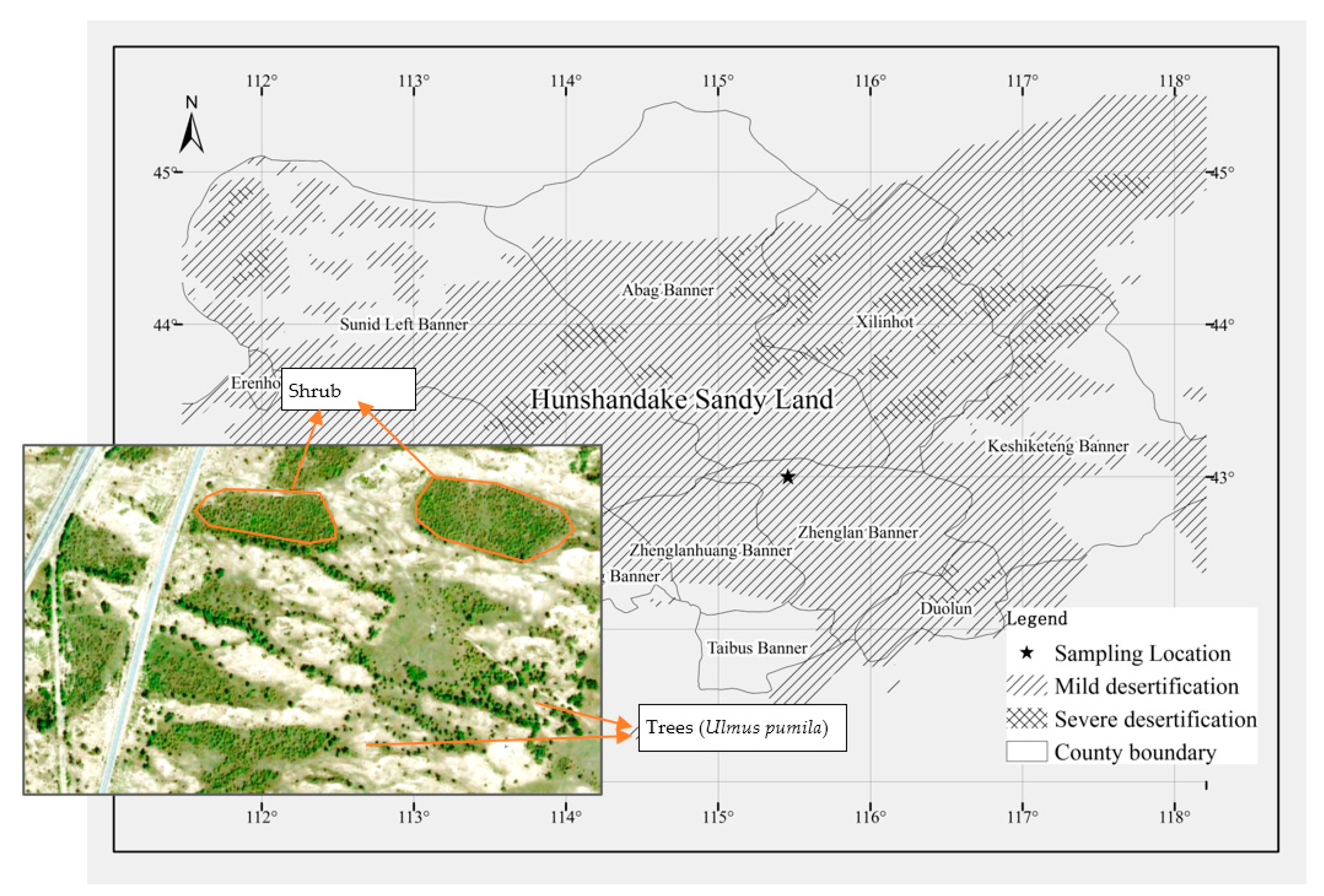
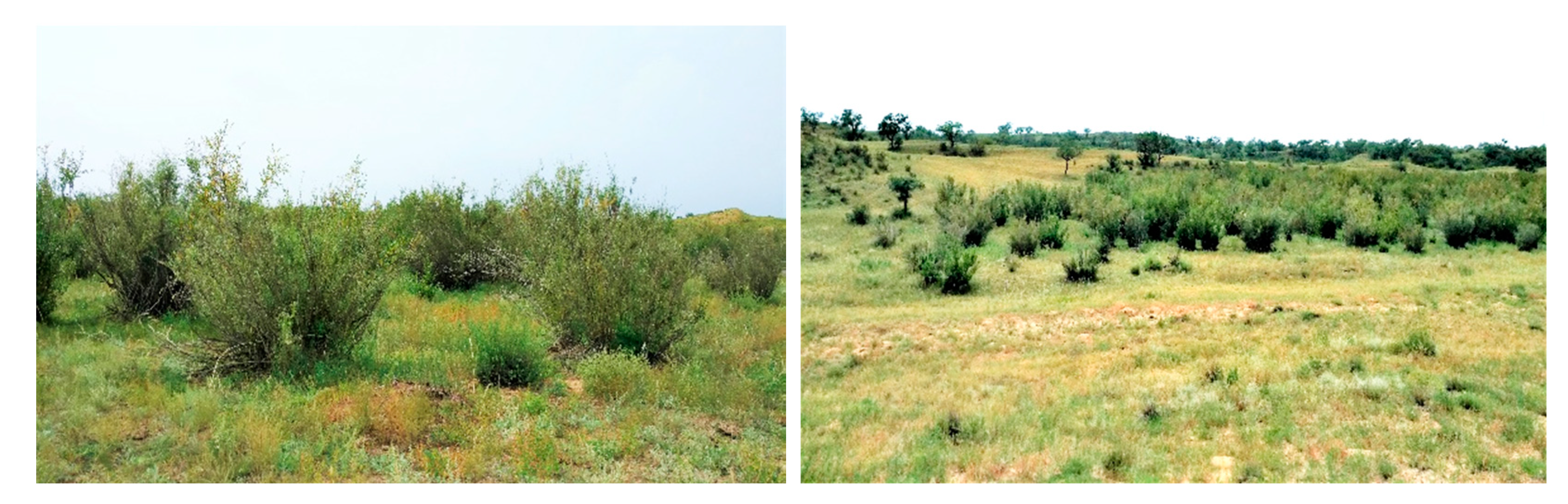
2.1. Study Area

The region of Hunshandake Sandy Land is in the middle of the Inner Mongolia Autonomous Region, which covers an area of 18,000 km² (42°–44° N, 113°–118° E) (Figure 1). The Sandy Land belongs to the eastern part of the desert belt in northern China, which stretches across the sub-humid, semi-arid, and arid climate zones. The average annual temperature is 0.9 °C–5.5 °C, the average yearly precipitation is 250–400 mm, and the annual evaporation is 2000–2700 mm. More than 98% of dunes are fixed or semi-fixed by vegetation. The Ulmus pumila woodland is the native top plant community in the Hunshandake Sandy Land, which is the most widely distributed, especially in the central and eastern regions. Ulmus pumila is the only tree species in the study area, concentrated on the shady slopes of sand dunes and scattered on the gentle slope between the dunes. Under the canopy of the trees, the lack of typical shade-tolerant undergrowth cannot form a real forest environment. Shrubs are distributed mainly in the depressions between sand dunes, where better water conditions are available. Ribes (Ribes diacantha Pall.) (S1), Betula (Betula fruticose Pall.) (S2), Red willow (Salix microstachya Turcz.) (S3) are the dominant species. The associated species include Hedysarum (Hedysarum mongolicum Turcz.), Ostryopsis (Ostryopsis davidiana Decne.), and Periploca (Periploca sepium Bunge.). These shrub species are tall, mixed in depressions, forming large shrub patches (Figure 1). Caragana (Caragana microphylla Lam.) (S4), Spiraea (Spiraea aquilegifolia Pall.) (S5) are smaller, often mixed on the shady slope, forming small patches of shrubs. Yellow willow (Salix flavida Chang et Skv.) (S6), usually scattered over bare sand, are pioneer plants for fixing sand dunes. The shrub community patches typically occupy a large area and stand out in the landscape of Hunshandake Sandy Land (Figure 2).

2.2. Above-Ground Biomass Sampling

The sample site had been built since 2013, about 100 hectares. All shrubs identified inside the sample site were measured, yielding a total of 30,000 individuals. The six dominant shrub species S1 to S6 were selected as samples, and averages of 20 individuals per species were randomly selected to cover the range of possible plant sizes. Five variables were measured for each individual plant using a long rod with scale: total height (h, cm), which is defined as the distance between the ground surface and highest crown point; maximum crown diameter (a₁, cm) and its perpendicular diameter (b₁, cm); and maximum diameter at the base (a₂, cm) and its perpendicular diameter (b₂, cm) (Figure 3). The maximum crown diameter was measured at the height where the crown width can be seen to be the largest. The maximum diameter at the base was measured at ground level, using a long rod with scale through bush branches.

The total above-ground live biomass (with leaves) of the 20 shrubs per species were harvested, weighed with a hanging scale (Nops Goldenlark OEM BT-203, accuracy = 0.01 kg), and recorded. A certain proportion of each individual’s branches were stored in plastic bags as samples. The samples were transported to a laboratory and dried in an air-forced oven at 80 °C until constant weight. Each individual’s water content was then calculated to convert fresh weight into dry weight, and the dry weight was used in the biomass models in this study. The descriptive statistics of the shrub measurements and the biomass data were shown in

Table 1. Descriptive statistics of the harvested shrubs.

Shrub Species	Height Range (cm)	Crown Diameter Range (cm)	Ground Diameter Range (cm)	Dried Biomass Range (g)
S1	80–190	43–250	13–107	130–7350
S2	180–380	90–335	18–131	450–14,380
S3	160–330	110–440	18–192	740–43,180
S4	55–140	60–280	17–243	120–5180
S5	55–170	60–215	22–84	160–1970
S6	150–340	52–455	14–296	340–3080

.

2.3. The Seven Models for Estimating Above-Ground Biomass of Shrub

Seven estimation methods for shrub biomass were classified into two kinds of fitting strategies. The models in the first kind were based on allometric models with single measurements as predictors, namely, total height (H), crown diameter (CD), and ground diameter (GD). Models in the second kind were based on allometric models with four different volumes as predictors, namely, V1, which was the volume of a circular cylinder with CD as the diameter; V2, which was the volume of a circular cylinder with GD as the diameter; V3, which was the volume of an elliptical cylinder with a1 and b1 as the long and short diameters, respectively; and V4, which was the volume of an inverted cone frustum with CD and GD as the long and short diameters, respectively. The mathematical expressions of these predictors were presented in

Table 2. Mathematical expressions of the seven predictors for shrub biomass estimation.

Code	Name	Formula
H	Height	H = h
CD	Crown Diameter	CD = (a1+ b1)/2
GD	Ground Diameter	GD = (a2 +b2)/2
V1	Circular Cylinder	V1 = πCD2h/4
V2	Circular Cylinder	V2 = πGD2h/4
V3	Elliptical Cylinder	V3 = πa1b1h/4
V4	Inverted Cone Frustum	V4 = 1/12πh(CD2 + CD × GD + GD2)

The formula’s parameters correspond to the parameters in Figure 3. a₁ is the maximum crown diameter, and b₁ is its perpendicular diameter, a₂ is the maximum ground diameter, and b₂ is its perpendicular diameter.

, and the geometric representations are shown in Figure 3.

Separate H and CD measurements were selected because they were the basic measurements of shrubs and popularly used in studies [25,30]. V1, V2, and V3 were selected because they were widely used in research and had definite geometric significance [7,12,31]. In this study, V4 has more geometries similar to actual shrubs and was introduced as a new predictor to improve estimation accuracy.

To obtain the most accurate biomass estimation models, initially, the main model forms, including linear, exponential, logarithmic, and power function proposed in the literature, were tested [19,25,32,33]. Finally, power function was selected to establish the allometric models because it generally performed well for all the six shrub species and predictors:

$$\mathrm{y}={\mathrm{ax}}^{\mathrm{b}}$$

(1)

where y is the above-ground shrub biomass, x is the predictor reflecting shrub size, a and b are the regression coefficients.

2.4. Regression Fitting and Accuracy Evaluation of the Seven Models

The Pearson’s correlation coefficients between the predictors and the biomass were calculated to observe each predictor’s estimation capability preliminarily. According to the bias-corrected Akaike Information Criterion (AICc), the best statistical model was selected, a likelihood criterion that penalizes the number of parameters [34]. We also reported the Coefficient of determination (R²), Root Mean Square Error (RMSE), and the regression’s p-value as alternative statistics reflecting the fitting accuracy.

Akaike Information Criterion (AIC) has been widely accepted for measuring the goodness of fit within a cohort of nonlinear models and frequently used for model selection [7,25,34,35]:

$$\mathrm{AIC}=-2\ln \left(\mathrm{L}\right)+2\mathrm{p}$$

(2)

where p is the number of parameters and ln(L) is the maximum log-likelihood of the estimated model.

To provide a fair playing ground, we employed an AIC variant that corrects for small sample sizes, the bias-corrected AIC (AICc) [34,35]:

$$\mathrm{AICc}=\mathrm{AIC}+\frac{2\mathrm{p}\left(\mathrm{p}+1\right)}{\mathrm{n}-\mathrm{p}-1}$$

(3)

where n is the sample size and p is the number of parameters.

The best statistical model with the highest R² and lowest SEE and AICc was selected [7,12,32]. All the statistical analyses were processed using IBM SPSS Statistics (Version 25.0, Armonk, NY, USA).

3. Results

3.1. Correlation Analysis between Predictors and Shrub Biomass

Pearson’s correlation coefficients preliminarily indicated each predictor’s estimation ability for shrub biomass, which were shown in

Table 3. Pearson’s correlation coefficients of predictors and biomass for the six shrub species.

Shrub Species	Predictors
	H	CD	GD	V1	V2	V3	V4
S1	0.54 *	0.83 **	0.81 **	0.83 **	0.81 **	0.88 **	0.91 **
S2	0.48 *	0.68 **	0.47 *	0.68 **	0.63 **	0.70 **	0.79 **
S3	0.74 **	0.83 **	0.77 **	0.92 **	0.88 **	0.91 **	0.95 **
S4	0.29	0.71 **	0.62 **	0.72 **	0.72 **	0.77 **	0.87 **
S5	0.63 **	0.76 **	0.51 *	0.66 **	0.71 **	0.70 **	0.71 **
S6	0.63 **	0.85 **	0.75 **	0.92 **	0.82 **	0.94 **	0.89 **
Average	0.55	0.78	0.66	0.79	0.76	0.82	0.85

* Correlation is significant at 0.05 level 2-tailed; ** Correlation is significant at 0.01 level 2-tailed.

. Among the three single measurements (H, CD, and GD), CD had the highest correlation coefficient with the six shrub species’ biomass, and this result was consistent with previous research [25,30]. Compared with the single measurements, the volume models V1, V3, and V4 had a better correlation with shrub biomass in general. Among all the predictors, the improved volume model V4 obtained the highest correlation with shrub biomass.

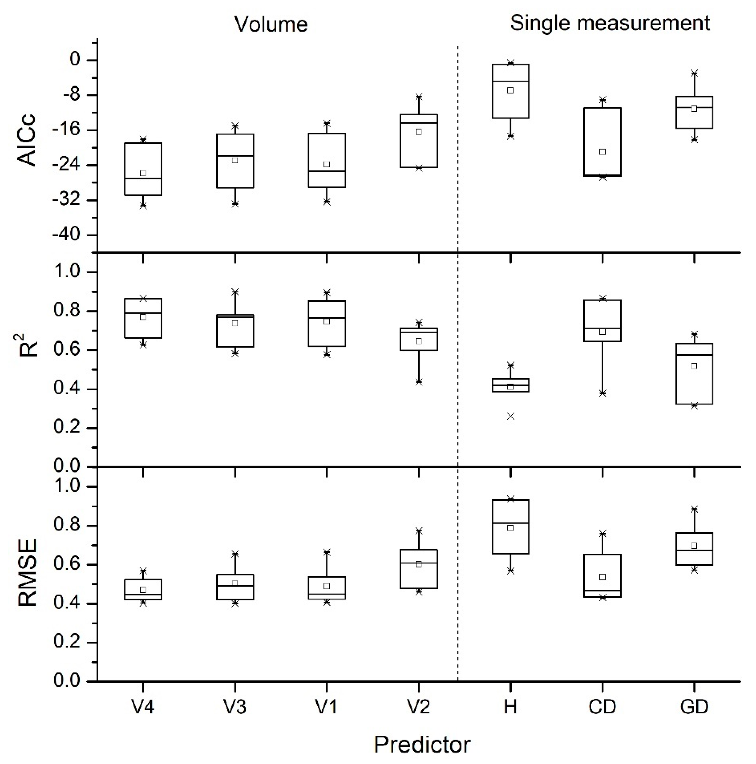
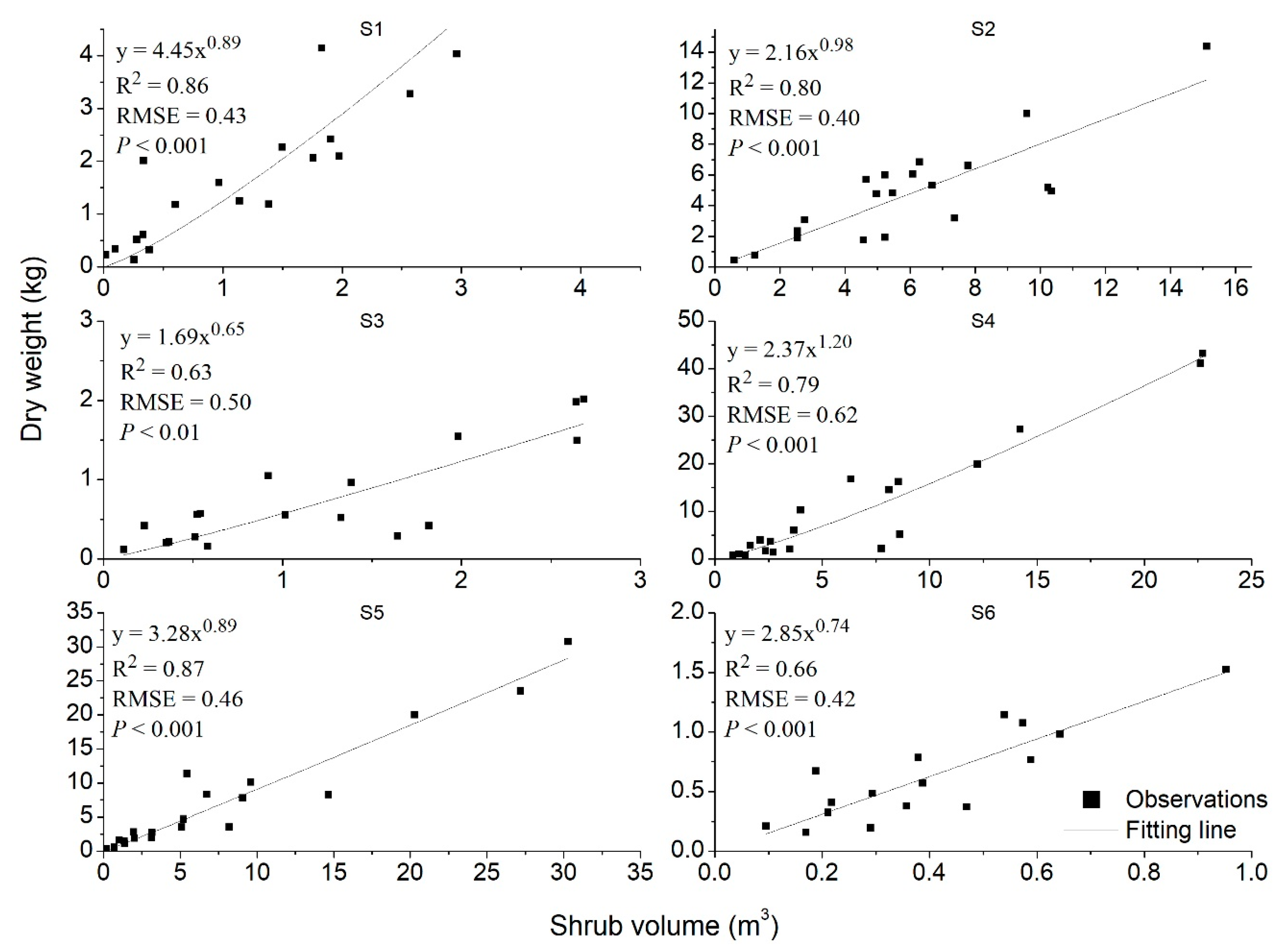
3.2. Fitting Accuracy Evaluation of the Seven Models

Based on the allometric model (Equation (1)), seven fitting models including different variables were established as predictors, and the model parameters are shown in

Table 4. Fitting parameters of the seven allometric models for the six shrub species.

Shrub Species	Predictors	a	b	AICc	R2	RMSE	p-Value
S1	H	1.00	2.84	−0.86	0.39	0.92	< 0.01
	CD	1.00	2.06	−26.47	0.87	0.43	<0.001
	GD	1.00	1.65	−11.88	0.68	0.66	<0.001
	V1	2.16	0.87	−25.01	0.85	0.45	<0.001
	V2	225.83	0.77	−15.48	0.74	0.60	<0.001
	V3	2.50	0.71	−18.23	0.78	0.55	<0.001
	V4	4.45	0.89	−26.39	0.86	0.43	<0.001
S2	H	1.00	3.10	−12.98	0.45	0.66	<0.01
	CD	1.00	2.37	−26.20	0.74	0.46	<0.001
	GD	1.02	1.30	−17.95	0.59	0.57	<0.001
	V1	1.42	1.00	−28.76	0.77	0.42	<0.001
	V2	37.43	0.68	−24.39	0.71	0.48	<0.001
	V3	1.43	1.00	−28.89	0.77	0.42	<0.001
	V4	2.16	0.98	−30.59	0.80	0.40	<0.001
S3	H	1.00	1.92	−8.03	0.26	0.71	0.052
	CD	1.00	1.25	−10.64	0.38	0.65	<0.05
	GD	1.02	0.72	−9.17	0.31	0.69	<0.05
	V1	1.47	0.78	−16.42	0.58	0.54	<0.01
	V2	1.95	0.43	−12.10	0.44	0.62	<0.01
	V3	1.47	0.78	−16.57	0.58	0.54	<0.01
	V4	1.69	0.65	−17.72	0.63	0.50	<0.01
S4	H	1.00	4.29	−0.70	0.52	0.93	<0.001
	CD	1.00	2.71	−8.83	0.68	0.76	<0.001
	GD	1.01	1.60	−2.69	0.57	0.89	<0.001
	V1	1.44	1.21	−14.17	0.76	0.67	<0.001
	V2	172.04	0.80	−8.06	0.67	0.78	<0.001
	V3	1.44	1.22	−14.75	0.76	0.66	<0.001
	V4	2.37	1.20	−16.76	0.79	0.62	<0.001
S5	H	1.00	3.51	−0.31	0.45	0.94	<0.01
	CD	1.00	2.12	−25.91	0.86	0.48	<0.001
	GD	1.01	1.33	−8.09	0.63	0.76	<0.001
	V1	1.88	0.96	−32.11	0.90	0.41	<0.001
	V2	24.13	0.66	−12.71	0.71	0.68	<0.001
	V3	1.91	0.96	−32.63	0.90	0.40	<0.001
	V4	3.28	0.89	−27.03	0.87	0.46	<0.001
S6	H	1.00	1.44	−17.04	0.39	0.57	<0.01
	CD	1.00	1.92	−26.25	0.64	0.43	<0.001
	GD	1.00	1.36	−15.33	0.32	0.60	<0.05
	V1	1.90	0.66	−25.13	0.62	0.45	<0.001
	V2	18.83	0.81	−24.22	0.60	0.46	<0.001
	V3	1.91	0.65	−24.95	0.62	0.45	<0.001
	V4	2.85	0.74	−27.23	0.66	0.42	<0.001

The mathematical structure and the model parameters are the same as the Formula (1).

. The block diagram in Figure 4 showed the mean and variation range of AICc, R², and RMSE, indicating the fitting accuracy and the fitting stability of different shrub species. Among the seven fitting models, the volume models (except V2) performed best, with lower AICc, and an average R² > 74%, RMSE < 0.50. V2 did not perform as well as the other three volume models, which may be related to the weak correlation between GD and shrub biomass (Table 3). V4 further improved the fitting accuracy with average higher R², lower AICc, and RMSE compared to V1 and V3. The variation of R², AICc and RMSE of V4-biomass models were relatively small across the six shrub species, which indicated that the V4-biomass model had a more stable fitting accuracy for different shrub species. Among the three single measurements, CD (average R² > 69%, RMSE < 0.54, AICc < −20) performed relatively better than H and GD (average R² < 52%, RMSE > 0.70, AICc > −11). Nevertheless, compared to the volume-biomass models (except V2), the AICc, R², and RMSE of CD-biomass models had a large variation across the six shrub species, suggesting that the CD-biomass model may not be accurate when fitting some shrub species.

Correlation analysis and fitting accuracy assessment showed that the V4-biomass allometric model best-estimated shrub biomass among the seven models. The fitting curves and parameters of the V4-biomass allometric models for the six species were shown in Figure 5. All equations were statistically significant (p < 0.01), and R² indicated that the models explained 63%–86% of biomass variability for the six shrub species. RMSE showed that approximately 95% of the observations fell within ±1.23% (double RMSE) of the fitting line.

4. Discussion

In recent years, with the attention to global warming and the carbon cycle, more and more researchers have begun to estimate the carbon sequestration capacity of vegetation in arid regions, where the vegetation is generally dominated by shrubs herbs [36]. It is first necessary to estimate the shrubs’ biomass more accurately to study shrubs’ carbon sequestration capacity [4]. However, the current shrub biomass estimation methods are not yet mature, and most of them are derived from the methods of tree biomass estimation. For trees, a single measurement such as diameter at breast height or height can generally get better prediction results, but this does not apply to shrubs because the shape of shrubs is very different from that of trees, and the shape of shrubs is more variable. Therefore, various compound predictors have appeared to meet researchers’ needs for shrub biomass estimation [30,33].

Nevertheless, researchers are easily confused when choosing among predictors because the studied shrub species may be very different, and it is hard to determine which predictor is suitable. This research attempts to find and improve predictors that are suited to different shrub species. Therefore, we selected six shrub species with different shapes and sizes and tested the performance of seven predictors for biomass estimating, including the new predictor (V4) that we improved ourselves.

Among the seven predictors, the single measurements performed relatively poorly compared to the volume models. Brown [37] established a suitable relationship between individual stem diameter and biomass for shrubs in northern Rocky Mountain. Still, in our study, it was impractical to measure each stems’ basal diameter because shrub species in our study area usually had dozens of stems at the base. Hence, we used the diameter of the area occupied by the shrub stems on the ground as GD rather than the diameter of the individual shrub stems. Among the three single measurements, CD performed much better than GD and H according to correlation analysis, which was consistent with the results in many other studies [5,23]. However, all these three single measurements performed poorly in the fitting analysis. The error varied significantly, indicating that the models’ accuracy with single measurements for different shrub species is unstable. The reason might be that the morphology of the shrub species was quite different, and it was difficult to accurately characterize the size of the shrub with a single measurement. Therefore, compound predictors have to be considered when simulating shrub biomass.

Among the four compound predictors, V1, V3, and V4 performed well, showing a good correlation with biomass and high fitting analysis accuracy. The volume model V2 associated with GD did not perform as well as the three other volume models, which was related to the weak correlation between GD and biomass (Table 3). V1 and V3, which are associated with CD, performed much better in biomass estimation, consistent with the strong correlation between CD and biomass. Conti et al. [24] also confirmed the superior performance of CD-related variables in estimating shrub biomass in their studies.

Murray and Jacobson [12] believed that surface areas and volumes could be derived from individual plants’ shapes, thereby further improving the development of biomass predictors for shrub species. Sternberg & Shoshany [29] tried different volume models to improve the estimation accuracy of shrub biomass in Israel. In this study, the V4 biomass model showed the best fitting accuracy and stability for different shrub species. Our study’s six shrub species had significantly different shapes and sizes, and the V4 model showed a good fitting effect on most of them. This is because the geometry of the V4 model is flexible and can be adapted to different shrub shapes. For example, if the GD is close to 0, the geometric shape would be similar to an inverted cone.

Additionally, if the GD is less than the CD, it would be an inverted cone frustum; and if the GD is close to the CD, the geometric shape would be similar to a cylinder. These geometric shapes can satisfy most shrub morphology, suggesting that V4 can be more widely used in different shrub species. In many studies, target shrubs were often multiple species, while the shapes of different shrub species were very different. Therefore, researchers need to use different volume models to estimate all shrub species’ volume to obtain better biomass estimates. The flexibility of the V4 can satisfy volume simulation of different shrubs shapes, provided that we fully measure the shrubs according to the routine without worrying about the differences of individual shrubs. Hence, if V4 was used as the shrub volume estimation method, and then use the volume as a predictor to establish a V4-biomass model, the research method could be simplified, and a more accurate and reliable biomass estimate could be obtained.

However, V4 involved more variables, which may be considered laborious in practice. Thus, we believe that if shrub measurements are sufficient, V4 would be the best predictor for shrub biomass estimation. Otherwise, the crown-related volumes V1 and V3 would be appropriate predictors.

In this study, we uniformly adopted a power function to establish allometric models. However, the linear function is also a commonly used form of function, and the relationship between volume (V1, V3, V4) and shrub biomass also showed a good linear relationship in this study (Figure 5). This article focused on selecting predictors and did not discuss the form of functions in detail. However, we tested linear functions, exponential functions, logarithmic functions, and polynomial functions before choosing power functions to construct the allometric model. However, no matter which form of the function we chose, the goodness of fit was consistent with the law: crown-related volumes > CD > H > GD. Therefore, we believe that, in addition to the functional form, the selection of independent variables (predictors) is of great significance to the effectiveness of the model and should be paid enough attention.

5. Conclusions

Our study showed that the single measurements were not suitable for estimating shrub biomass. The crown-related volumes performed much better than single measurements when used as predictors of shrub biomass estimation. Among the crown-related volumes, the improved predictor, the volume of an inverted cone frustum with a crown diameter and ground diameter as the long and short diameters performed best according to fitting accuracy and stability of different shrub species. Consequently, we suggest that if studies involve various shrub species, and a general model is needed to accurately estimate shrub volume and then use the volume as a predictor of biomass estimation, the volume of an inverted cone frustum with a crown diameter and ground diameter as the long and short diameters would be an ideal choice.

References

1. White, R.P.; Nackoney, J. Drylands, People, and Ecosystem Goods and Services: A Web-Based Geospatial Analysis; World Resources Institute: Washington, DC, USA, 2003. [Google Scholar]
2. Hou, X.Y. Vegetation Map of the People’s Republic of China and Its Illustration; China Cartographic Publishing House: Beijing, China, 1982. (In Chinese) [Google Scholar]
3. Cerrillo, R.M.N.; Oyonarte, P.B. Estimation of above-ground biomass in shrubland ecosystems of southern Spain. For. Syst. 2006, 15, 197–207. [Google Scholar]
4. Daryanto, S.; Eldridge, D.J.; Throop, H.L. Managing semi-arid woodlands for carbon storage: Grazing and shrub effects on above- and belowground carbon. Agric. Ecosyst. Environ. 2013, 169, 1–11. [Google Scholar] [CrossRef]
5. Pasalodostato, M.; Ruizpeinado, R.; Rio, M.D.; Montero, G. Shrub biomass accumulation and growth rate models to quantify carbon stocks and fluxes for the Mediterranean region. Eur. J. For. Res. 2015, 134, 537–553. [Google Scholar] [CrossRef]
6. Ruizpeinado, R.; Moreno, G.; Juarez, E.; Montero, G.; Roig, S. The contribution of two common shrub species to above-ground and belowground carbon stock in Iberian dehesas. J. Arid. Environ. 2013, 91, 22–30. [Google Scholar] [CrossRef]
7. Yang, H.; Wang, Z.; Tan, H.; Gao, Y. Allometric models for estimating shrub biomass in desert grassland in northern China. Arid Land Res. Manag. 2017, 31, 283–300. [Google Scholar] [CrossRef]
8. Li, Y.; Jiang, G.; Gao, L.; Niu, S.; Liu, M.; Yu, S.; Peng, Y. Impacts of human disturbance on elms-motte-veldt in Hunshandak sandland. Acta Phytoecol. Sin. 2003, 27, 829–834. [Google Scholar] [CrossRef] [Green Version]
9. Wang, X.; Schaffer, B.E.; Yang, Z.; Rodrigueziturbe, I. Probabilistic model predicts dynamics of vegetation biomass in a desert ecosystem in NW China. Proc. Natl. Acad. Sci. USA 2017, 114, 201703684. [Google Scholar] [CrossRef] [Green Version]
10. Lin, J.; Wang, M.; Ma, M.; Lin, Y. Aboveground Tree Biomass Estimation of Sparse Subalpine Coniferous Forest with UAV Oblique Photography. Remote Sens. 2018, 10, 1849–1868. [Google Scholar] [CrossRef] [Green Version]
11. Gabrielle, N.B.; Emma, C.U.; Hugh, D.S. Estimating Biomass in California’s Chaparral and Coastal Sage Scrub Shrublands. Madroño 2018, 65, 28–46. [Google Scholar] [CrossRef]
12. Murray, R.B.; Jacobson, M.Q. An Evaluation of Dimension Analysis for Predicting Shrub Biomass. J. Range Manag. 1982, 35, 451. [Google Scholar] [CrossRef]
13. Rojo, V.; Arzamendia, Y.; Perez, C.; Baldo, J.L.; Vila, B.L. Double Sampling Methods in Biomass Estimates of Andean Shrubs and Tussocks. Rangel. Ecol. Manag. 2017, 70, 718–722. [Google Scholar] [CrossRef]
14. Vora, R.S. Predicting biomass of five shrub species in northeastern California. J. Range Manag. 1988, 41, 63–65. [Google Scholar] [CrossRef]
15. Ximenes, F.; Kathuria, A.; Mclean, M.; Coburn, R.; Sargeant, D.; Ryan, M.; Williams, J.; Boer, K.; Mo, M. Carbon in Mature Native Forests in Australia: The Role of Direct Weighing in the Derivation of Allometric Equations. Forests 2018, 9, 60. [Google Scholar] [CrossRef] [Green Version]
16. Ludwig, J.A.; Reynolds, J.F.; Whitson, P.D. Size-biomass Relationships of Several Chihuahuan Desert Shrubs. Am. Midl. Nat. 1975, 94, 451–461. [Google Scholar] [CrossRef]
17. Mason, N.W.H.; Beets, P.N.; Payton, I.J.; Burrows, L.E.; Holdaway, R.J.; Carswell, F.E. Individual-Based Allometric Equations Accurately Measure Carbon Storage and Sequestration in Shrublands. Forests 2014, 5, 309–324. [Google Scholar] [CrossRef] [Green Version]
18. Chave, J.; Rejoumechain, M.; Burquez, A.; Chidumayo, E.N.; Colgan, M.S.; Delitti, W.B.C.; Duque, A.; Eid, T.; Fearnside, P.M.; Goodman, R.C. Improved allometric models to estimate the above-ground biomass of tropical trees. Glob. Chang. Biol. 2014, 20, 3177–3190. [Google Scholar] [CrossRef]
19. Ganeshamurthy, A.N.; Ravindra, V.; Venugopalan, R.; Mathiazhagan, M.; Bhat, R.M. Biomass Distribution and Development of Allometric Equations for Non-Destructive Estimation of Carbon Sequestration in Grafted Mango Trees. J. Agric. Sci. 2016, 8, 201. [Google Scholar] [CrossRef] [Green Version]
20. Ploton, P.; Barbier, N.; Momo, S.T.; Rejoumechain, M.; Bosela, F.B.; Chuyong, G.; Dauby, G.; Droissart, V.; Fayolle, A.; Goodman, R.C. Closing a gap in tropical forest biomass estimation: Taking crown mass variation into account in pantropical allometries. Biogeosciences 2016, 13, 1571–1585. [Google Scholar] [CrossRef] [Green Version]
21. Rutishauser, E.; Nooran, F.; Laumonier, Y.; Halperin, J.; Rufiie; Hergoualch, K.; Verchot, L.V. Generic allometric models including height best estimate forest biomass and carbon stocks in Indonesia. For. Ecol. Manag. 2013, 307, 219–225. [Google Scholar] [CrossRef]
22. Jagodzinski, A.M.; Dyderski, M.K.; Gesikiewicz, K.; Horodecki, P. Tree- and Stand-Level Biomass Estimation in a Larix decidua Mill. Chronosequence. Forests 2018, 9, 587. [Google Scholar] [CrossRef] [Green Version]
23. Zhang, L.; Cui, G.; Shen, W.; Liu, X. Cover as a simple predictor of biomass for two shrubs in Tibet. Ecol. Indic. 2016, 64, 266–271. [Google Scholar] [CrossRef]
24. Conti, G.; Enrico, L.; Casanoves, F.; Díaz, S. Shrub biomass estimation in the semi-arid Chaco forest: A contribution to the quantification of an underrated carbon stock. Ann. For. Sci. 2013, 70, 515–524. [Google Scholar] [CrossRef] [Green Version]
25. Huff, S.; Ritchie, M.W.; Temesgen, H. Allometric equations for estimating above-ground biomass for common shrubs in northeastern California. For. Ecol. Manag. 2017, 398, 48–63. [Google Scholar] [CrossRef]
26. Yi, T.; Arshad, A.; Li, H. Bayesian model predicts the above-ground biomass of Caragana microphylla in sandy lands better than OLS regression models. J. Plant. Ecol. 2020, 13, 732–737. [Google Scholar]
27. Picard, N.; Rutishauser, E.; Ploton, P.; Ngomanda, A.; Henry, M. Should tree biomass allometry be restricted to power models. For. Ecol. Manag. 2015, 353, 156–163. [Google Scholar] [CrossRef]
28. Uso, J.L.; Mateu, J.; Karjalainen, T.; Salvador, P. Allometric regression equations to determine aerial biomasses of Mediterranean shrubs. Plant Ecol. 1997, 132, 59–69. [Google Scholar] [CrossRef]
29. Sternberg, M.; Shoshany, M. Influence of slope aspect on Mediterranean woody formations: Comparison of a semi-arid and an arid site in Israel. Ecol. Res. 2001, 16, 335–345. [Google Scholar] [CrossRef]
30. Ma, Y.; Li, G.; Pan, Y.; Ma, Y.; Wang, Q.; Zhang, C. Prediction model for biomass of 3 shrubs in Hunshandake sandy land. J. Arid. Lan. Res. Envi. 2017, 31, 198–201. [Google Scholar]
31. Hierro, J.L.; Branch, L.C.; Villarreal, D.; Clark, K.L. Predictive equations for biomass and fuel characteristics of Argentine shrubs. J. Range Manag. 2000, 53, 617–621. [Google Scholar] [CrossRef]
32. He, A.; Mcdermid, G.J.; Rahman, M.M.; Strack, M.; Saraswati, S.; Xu, B. Developing Allometric Equations for Estimating Shrub Biomass in a Boreal Fen. Forests 2018, 9, 569. [Google Scholar] [CrossRef] [Green Version]
33. Flade, L.; Hopkinson, C.; Chasmer, L. Allometric Equations for Shrub and Short-Stature Tree Aboveground Biomass within Boreal Ecosystems of Northwestern Canada. Forests. 2020, 11, 1207. [Google Scholar] [CrossRef]
34. Spiess, A.N.; Neumeyer, N. An evaluation of R2 as an inadequate measure for nonlinear models in pharmacological and biochemical research: A Monte Carlo approach. BMC Pharmacol. 2010, 10, 6. [Google Scholar] [CrossRef] [PubMed] [Green Version]
35. Erik, V.; Kian, W.C. Carbon storage estimation of tropical urban trees by an improved allometric model for above-ground biomass based on terrestrial laser scanning. Urban. For. Urban. Gree. 2019, 44, 126387. [Google Scholar]
36. IPCC. Contribution of Working Groups I, II and III to the Fifth Assessment Report of the Intergovernmental Panel on Climate Change. In Climate Change 2014; Synthesis Report; Core Writing Team, Pachauriand, R.K., Meyer, L.A., Eds.; IPCC: Geneva, Switzerland, 2014; p. 151.z. [Google Scholar]
37. Brown, J.K. Estimating shrub biomass from basal stem diameters. Can. J. For. Res. 1976, 6, 153–158. [Google Scholar] [CrossRef]
Figure 1. Location of the study site and the landscape of the sample plot (The photo was taken by drone in May 2018).
Forests 12 00167 g001
Figure 2. Field photos of the sample plot (The photos were taken in August 2018).
Forests 12 00167 g002
Figure 3. Geometric configurations of the four volume models (h is the total height; a1 and b1 are the crown orthogonal cross axes; a2 and b2 are the basal stems orthogonal cross axes; (V1V4) represent the four volume models).
Forests 12 00167 g003
Figure 4. Box chart of AICc, R2, and RMSE of the seven models in shrub biomass fitting.
Forests 12 00167 g004
Figure 5. V4—biomass linear fit models for the six shrub species. (S1–S6 represents the six shrub species.)
Forests 12 00167 g005