Development of a Modality-Invariant Multi-Layer Perceptron to Predict Operational Events in Motor-Manual Willow Felling Operations

Abstract

Motor-manual operations are commonly implemented in the traditional and short rotation forestry. Deep knowledge of their performance is needed for various strategic, tactical and operational decisions that rely on large amounts of data. To overcome the limitations of traditional analytical methods, Artificial Intelligence (AI) has been lately used to deal with various types of signals and problems to be solved. However, the reliability of AI models depends largely on the quality of the signals and on the sensing modalities used. Multimodal sensing was found to be suitable in developing AI models able to learn time and location-related data dependencies. For many reasons, such as the uncertainty of preserving the sensing location and the inter- and intra-variability of operational conditions and work behavior, the approach is particularly useful for monitoring motor-manual operations. The main aim of this study was to check if the use of acceleration data sensed at two locations on a brush cutter could provide a robust AI model characterized by invariance to data sensing location. As such, a Multi-Layer Perceptron (MLP) with backpropagation was developed and used to learn and classify operational events from bimodally-collected acceleration data. The data needed for training and testing was collected in the central part of Romania. Data collection modalities were treated by fusion in the training dataset, then four single-modality testing datasets were used to check the performance of the model on a binary classification problem. Fine tuning of the regularization parameters (α term) has led to acceptable testing and generalization errors of the model measured as the binary cross-entropy (log loss). Irrespective of the hyperparameters’ tunning strategy, the classification accuracy (CA) was found to be very high, in many cases approaching 100%. However, the best models were those characterized by α set at 0.0001 and 0.1, for which the CA in the test datasets ranged from 99.1% to 99.9% and from 99.5% to 99.9%, respectively. Hence, data fusion in the training set was found to be a good strategy to build a robust model, able to deal with data collected by single modalities. As such, the developed MLP model not only removes the problem of sensor placement in such applications, but also automatically classifies the events in the time domain, enabling the integration of data collection, handling and analysis in a simple less resource-demanding workflow, and making it a feasible alternative to the traditional approach to the problem.

1. Introduction

Short-rotation willow crops (SRWC) are seen nowadays as a valuable alternative to produce renewable energy, contributing also to the rural development, job market diversification, carbon sink, biodiversity and diversification of agricultural crops and bio-products. They are commonly established on agricultural lands and share many features with the traditional forestry, in particular the silvicultural practices [1]. Moreover, willow was found to be suitable for other engineering purposes, commonly exhibiting features such as a rapid growth rate, high biomass production, increased coppicing ability and tolerance to high planting densities [2].

When grown to produce biomass as a feedstock for the energy industry, one of the final SRWC production steps consists of harvesting operations. Several fully-mechanized operational systems were developed, tested and are currently in use for large-scale commercial willow harvesting purposes [3,4]. Still, the increased costs associated with harvesting operations [5] are seen as a limiting factor of profitability, which requires optimization [6]. While other operations which are common to SRWC cultivation can be done directly by their owners using equipment and machines of general agricultural purpose, it has been shown that, irrespective of the SRWC scale, the farmers cannot afford to own and operate expensive harvesting equipment [3,5]. In many cases, the lack or the limited availability of such equipment [7] has been tackled by the use of motor-manual means [8,9], which seem to be more adapted to harvesting operations carried out on small and dispersed plots [10], especially in those geographic regions in which the cost of the manual labor is still affordable, and may compensate for lower productivities [11].

Irrespective of the harvesting system used, its optimization requires at least data on production outputs and resources used (i.e., time, fuel, money) [12], and it is quite typical to implement time studies to evaluate its operational performance [13] as a common input for optimization. There are many examples, including those referenced in this paper, of using time-and-motion studies to evaluate the performance of operations. Unfortunately, most of the currently used methods to get time consumption data are resource intensive [14], requiring qualified personnel and specific logistics to collect, process, analyze and interpret it.

In relation to the use of motor-manual equipment to harvest SRWCs, some progress has been made by the use of dataloggers equipped with acceleration sensors to automate field data collection, which was then coupled with Global Positioning System’s (GPS) data to infer the operational behavior in such operations [7,10]. In those studies, the analytical procedures of accounting and categorizing the time consumption on operational tasks were done by human intervention, requiring prior knowledge of the process mechanics and sensors’ response and, more importantly, a hands-on approach to data processing, summarization and categorization. To eliminate much of that effort, Artificial Intelligence (AI) techniques have been lately used for a number of applications with excellent results in the recognition and classification of operational time, based on signals produced by various sensors, including accelerometers [15,16,17,18]. Nevertheless, the applicability of the developed models stays well inside their intended application, mainly due to the labelling outcomes, which are application-specific, and to the sensing modality which could produce contrasting responses in magnitude, calling for the location preservation when using unimodal sensing designs [17,18]. To this end, a sensing modality could be characterized by the type of physical parameter measured by a sensor and by the location of sensing it on a given study object. As such, multimodal sensing may involve the use of at least two sensors measuring the same physical parameter at different locations or the use of at least two sensors measuring different physical parameters at the same location.

Going back to the use of accelerometers to collect signals which may be useful for operational activity recognition in motor-manual felling of willow, unimodal sensing becomes important to save resources, and the use of a single sensor is desirable and affordable. However, there are many possible locations in which an accelerometer could be placed on a given tool, such as a brush cutter, making it likely to get signals characterized by a high variability in magnitude due to the sensing location. In addition, there is a high variability given by the operational conditions themselves, which may change even in the same harvested plot, and by the operational behavior of the workers. In such conditions, the models developed by training an AI algorithm need to have an acceptable generalization ability, in such a way that at least the location of signal collection would become irrelevant for a given classification algorithm. In our knowledge, a robust model able to reliably deal with unimodally sensed acceleration signals, i.e., acceleration sensed at a single location on the tool irrespective of the location, was not studied so far, while developing it from multimodally sensed data could help overcome the limitations stated above; if such a model would prove to be reliable irrespective of the sensing location, then it will contribute to resource saving while easing the data collection, handling and analysis workflow.

The goal of this study was to develop a modality-invariant operational prediction model with application in motor-manual felling of willow by brush cutters. The problem was approached by the means of training and testing a Multi-Layer Perceptron (MLP) with backpropagation on acceleration signals. Acknowledging that there could be many other approaches to the problem, the choice of the MLP as a technique to be used, as well as of the acceleration data as input signals, was mainly based on the author’s experience with the MLP algorithms and the availability of acceleration signal data; in addition, the choice was guided by the findings of recent work, repeatedly showing excellent results in task recognition applications when using acceleration signals as inputs in the AI algorithms. By a modality-invariant model we are referring to a model able to acceptably generalize from any acceleration signal collected by the same sensor type, anywhere of an observed tool, while preserving the highest possible classification performance and the lowest possible generalization error.

2. Materials and Methods

2.1. Data Collection

2.1.1. Study Location and Crop Layout

The data used in this study were collected in the center of Romania, from three locations (

Table 1. Locations of data collection and the summarized description of the datasets.

Location	Dataset a	Size b [s]	Date of Collection	Coordinates
Poian 1	TRAIN_E	18,377	04/11/2017	46°04.373′ N–26°10.924′ E
	TRAIN_S	18,377	04/11/2017	46°04.373′ N–26°10.924′ E
Poian 2	TEST_E1	26,493	02/27/2017	46°04.354′ N–26°10.904′ E
	TEST_S1	22,885	02/27/2017	46°04.354′ N–26°10.904′ E
Belani	TEST_E2	11,859	03/02/2017	46°03.362′ N–26°11.208′ E
	TEST_S2	9285	03/02/2017	46°03.362′ N–26°11.208′ E
TOTAL	-	107,276	-	-

Note: ^a TRAIN means that the dataset was used in the training phase of the MLP, TEST means that the dataset was used in the testing phase of the MLP, E means that the data was collected by datalogger placement on the tool’s engine, S means that the data was collected by the datalogger placement on the tool’s transmission shaft, 1 means that the dataset was the first of the same modality class, 2 means that the dataset was the second of the same modality class; ^b size refers to the number of one-second sampled observations retained in the training and testing datasets.

), where motor-manual willow felling operations were observed in the Spring of 2017. The plots taken into study were located in an intra-mountainous depression at an altitude of ca. 600 m a.s.l. The climate in the area is characterized by a strong continentalism with warm summers and cold winters. All the plots (Poian 1, Poian 2 and Belani, Covasna County, Romania) were planted according to the European willow planting layout, in which the planting is done in twin rows distanced at 75 cm, and each twin row is distanced at 1.5 m from the next one; commonly, the distance between the cuttings used for planting is of 60 cm [19].

Willow crops are becoming a common land use feature in the landscape of the study area, though they are typically established on small and dispersed plots whose previous use was agricultural [20]. In addition to the size and dispersion of the plots, the cultivation practice in the area is strongly influenced by the available technology for planting, cutback and harvesting operations, which are partly mechanized [7,9,10,19,20,21]; many of them, such as harvesting, are relying to a great extent on motor-manual operations which are usually done by the use of brush cutters [7,9,10]. This situation is often leading to practicing rotations of 2–3 years, and typical for the area is that motor-manual willow felling operations are done in the early spring. Most of the operations related to willow cultivation in the area are done by employing local people on a daily basis.

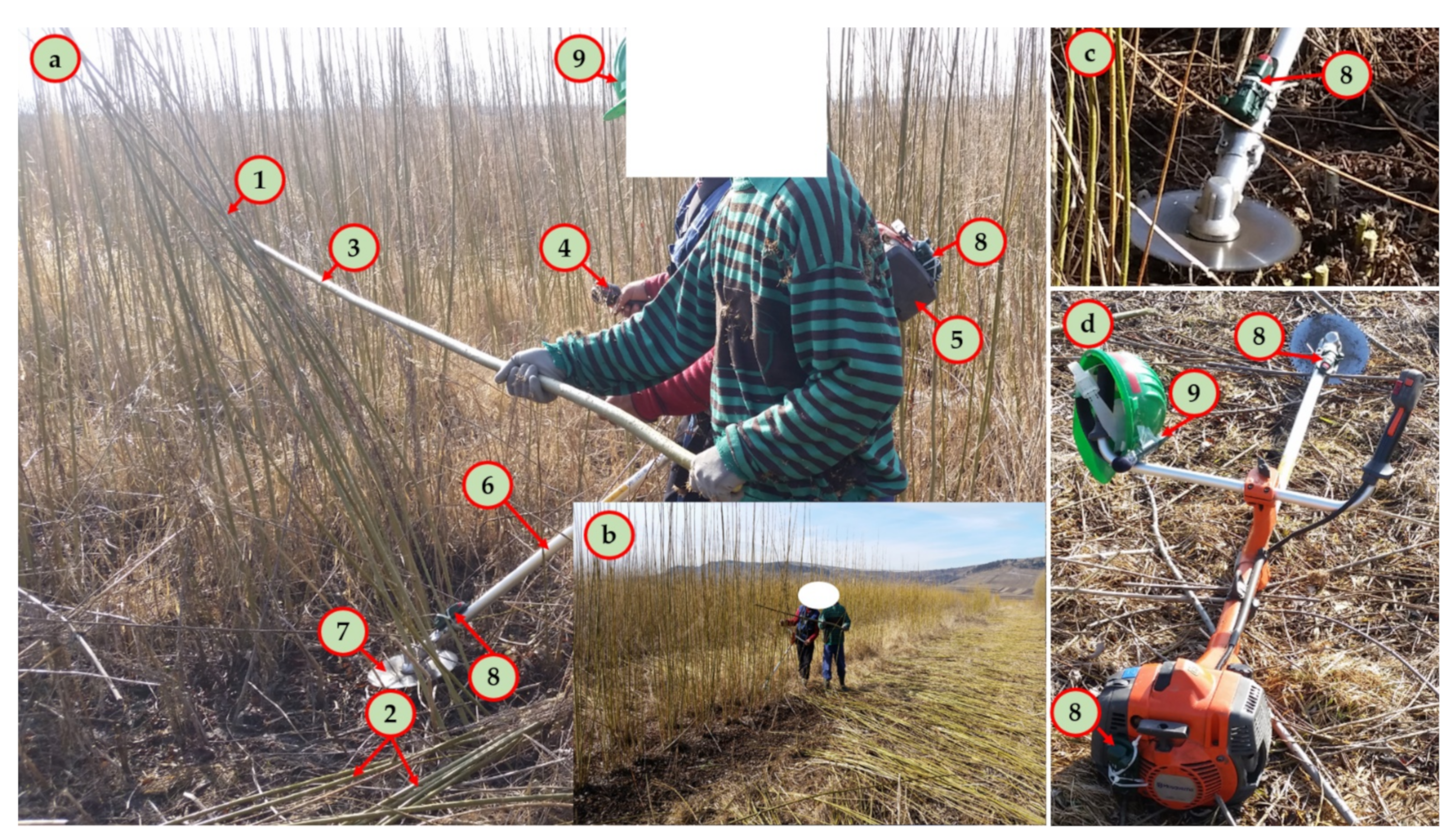
2.1.2. Tool Description, Work Organization and Relevant Process Mechanics

The tool used for felling was a brush cutter made by Husqvarna (Model 545 RX, Husqvarna AB, Stockholm, Sweden), featuring an engine output of 2.1 kW at 9000 rpm and a transmission shaft that enables the connection and power transfer between the engine and the cutting device (Figure 1); tools from this class are assumed to produce a noise level of 100 db(A) [22]. Harvesting work is typically done by motor-manual felling followed by manual bunching, transportation and chipping at a biomass terminal, or by bunching and chipping on site [23]. Brushcutters are commonly used in the study area to motor-manually fell the willow, being tools that can be adapted easily to a variety of jobs, simply by changing their active cutting devices [22,24]; when used for willow felling, they are usually equipped with steel saw blades (discs).

The felling work is commonly done by two workers (Figure 1) of which one is the brush cutter operator who is in charge of the mechanical felling tasks and tool maintenance, and the other one assists the felling by a wooden stick [7,9,10,19].

While being rather simple, the organization of felling work is influenced by the capability limits of the used tools, layout of the crops and weather conditions [7,19], and it needs to be done with much attention and caution to ensure the safety of both workers. As such, felling direction is commonly adopted toward the exterior of the crop, felling work is progressing on a single row (one of the twins), and in such cases in which the length of the crop is very long, transversal corridors are often practiced to shorten the distances covered per turn, to be able to refuel and maintain the tool [19]. The assistant needs to place himself at a considerable distance behind the feller and he interacts with the stems to be felled only by the wooden stick, while the feller needs to be able to coordinate and control his motions on very short trajectories. The relevant work elements which may occur in such operations are the effective on-row felling, moving at the headlands or on a transversal corridor to approach a new willow row at the opposite side of the crop, maintenance and refueling, rest and meal breaks, as well as other kind of delays [7,9]. The distinctive feature of these operations is that, excepting the felling, the rest of work elements are typically characterized by engine non-use. Therefore, monitoring the engine working time makes it possible to accurately monitor the main work time consumption, which stands for a category of time in which the direct transformation of the work object takes place [13], and which is also useful and important to account for the fuel intake as specific to motor-manual operations [24,25].

Looking at a finer scale, however, the felling consists of worker’s advancement on the row with various engine running regimes, combined with movements of the active cutting device of the tool toward outside and inside the crop to make the cuts, which are likely to produce variability in the responses given by the use of various sensors. Another relevant issue is the placement location of the dataloggers. For instance, accelerometer dataloggers could be placed at different locations on the engine block, as well as at different locations of the transmission shaft, therefore making it possible to receive different magnitudes of the acceleration during engine use; however, when the engine is switched off, the responses collected by accelerometers placed at different locations of the tool could be similar.

In the study area, felling work is always done by workers having an extensive experience in SRWC felling operations, gained on already more than a decade of SRWC management in Romania. Field data collection, which was done in 2017, was based on the informed consent of the observed workers and of the SRWCs’ owner. They were informed about the intended use of the data and agreed to be observed when performing their jobs.

2.1.3. Instrumentation

Two datalogger types were used to collect the field data used in this study. Acceleration response, as the main data stream used, was measured and recorded using two Extech^® VB300 triaxial dataloggers (Extech Instruments, FLIR Commercial Systems Inc., Nashua, NH, USA). Irrespective of the study location, the acceleration dataloggers were set by the use of the dedicated software to collect data in the motion detection mode (threshold of 1 g), at a sampling rate of one second. One of them was placed on the engine’s block and the other one was placed on the transmission shaft, at locations that were chosen carefully in such a way that they would not interfere with work safety. Both dataloggers were reinforced on the tool using highly-resistant plastic straps and were checked for holding before running the experiments and during the work breaks. An Extech^® 407,760 sound pressure level datalogger (Extech Instruments, FLIR Commercial Systems Inc., Nashua, NH, USA) was used to collect additional data needed for labelling purposes. It was set to continuously collect the sound pressure level on the dB(A) scale, at a sampling rate of one second, and it was placed on the helmet worn by the brush cutter operator. The main technical features of the used dataloggers are available on the producing company’s website [26,27]. Figure 1 shows the approach used to equip the tool and the worker with the used dataloggers.

2.1.4. Datasets

Six acceleration datasets were collected in the three locations taken into study (Table 1) and the intention was to get for each of them a time overlapping sound pressure level dataset. However, due to a battery malfunction, sound pressure level data was lost in the case of Belani location. By the construction and setup of the acceleration dataloggers, the data is collected and stored as discrete triaxial (X, Y and Z) time-labelled responses; they are further summarized in the form of vector magnitudes, also known as the Euclidian Norm (EN), which is some sort of data fusion [28], and which is enabled by the dedicated software. The EN, which is named by the dedicated software under the generic term of “vector sum”, may be written as in Equation (1) and it allows for a first normalization of the data, making it invariant to the axis movement. In fact, raw acceleration signals contain movement, gravity and noise components [29], while the instruments used to collect them respond well to vibration, a property which was used in this study.

$$A_i=\sqrt{x_i^2+ y_i^2+ z_i^2}$$

(1)

where A_i is a discrete value, in the form of Euclidian Norm (vector magnitude, vector sum), computed for a given sampling rate (adopted to one second in this study), and x_i, y_i and z_i are the accelerometer’s raw responses on the axis X, Y and Z, respectively, for the observation i.

Sound pressure level data was collected and outputted in a similar way, being time and date labelled, and showing the sound pressure level measured in dB(A) at a sampling rate set at one second. In addition, both dataloggers can output data in computer-friendly formats such as the Microsoft Excel^® (Microsoft, Redmond, WA, USA). CSV files, and both of them provide data ID’s and some summary statistics placed at the beginning of each file. Figure A1, Figure A2, Figure A3, Figure A4 and Figure A5 are showing the patterns of A_i in the datasets used for training and testing of the MLP, emphasizing the amplitude and magnitude differences due to the location of the datalogger and engine working regimes.

2.2. Data Preprocessing Workflow

2.2.1. Data Pairing, Segmentation and Labelling

To ease the effort of labelling the training data, as well as to compare the multimodal responses collected by the two acceleration dataloggers placed on the same tool, data pairing procedures were applied to the first two datasets (TRAIN_E and TRAIN_S) based on their time labels. This procedure was necessary to be able to label both datasets at once. Data pairing was done in Microsoft Excel^®, and it accounted for those observations which were present in both datasets and shared the same time label, an issue which was computationally approached, assessed and solved using logical functions. For example, if an observation from a given training dataset did not have had a corresponding time-labeled observation in the other training dataset, then it was deleted. This process was also run vice versa, until reaching a double set of observations sharing their time labels.

Labelling of the training datasets was done by considering the responses recorded by the acceleration and sound pressure level dataloggers (Figure 2), based on known experience on their responses in terms of magnitude. Two states were documented by labelling and segmentation, namely the engine running (labelled in the database by the string code ON) and the engine turned off (labelled in the database by the string code OFF).

For instance, sound pressure levels close to those described by the manufacturer for the operation of the tool (ca. 100 dB(A)) have pointed that the engine was on and throttled, therefore indicating that the worker was engaged in the effective felling operations. Drops in the magnitude of the sound pressure level (as shown in Figure 2 by the data labelled with 3), were considered to be the events in which the engine was on but no felling was done (idle running); these events were labelled as ON. Moreover, acceleration responses in the range of 1.1–3.0 g were compared to the data on sound pressure level, generally leading to their classification as engine OFF events. Transient events (Figure 2, data labelled by 5) were included in the engine working category as well. However, due to the acceleration data collection mode (motion detection) and pairing procedures used, which have led to some missing data, the sound pressure level dataset was paired by doing some adaptations in the time domain such as removing some data or moving some data segments to pair them with the acceleration data. This was done for approximately 10% of the joint dataset, then the patterns generated by the magnitude of acceleration data were used for further labelling.

Based on the experience gained during the labelling and segmentation tasks done on the training dataset, the distributions of data in specific patterns were used as a condition to label the data in the rest of the datasets, which were used for MLP testing (Figure A2, Figure A3, Figure A4 and Figure A5). Prior to the labelling and segmentation tasks, these datasets were preserved to their original number of observations, as they were outputted by the acceleration dataloggers. Therefore, the datasets shown in Figure A1, Figure A2, Figure A3, Figure A4 and Figure A5 contained the final number of one-second observations as described in Table 1, and each observation contained in them was the Euclidian Norm computed according to the Equation (1).

2.2.2. Fusion of the Training Datasets

All the datasets used in this study were subjected to early data fusion by the computation of Euclidian Norm. However, to simultaneously capture both the local dependencies over time and the spatial dependencies over modalities of collection, the approach was similar to that described in [30], and consisted of fusing the training datasets by a procedure referred as vertical stacking [28]. In particular, it was assumed that a more accurate data representation in the trained model, which could be achieved by the inclusion of spatial dependencies over the modalities of collection, could be important for the evaluation of datasets coming from other experiments using a single modality for field data collection, enhancing the trained model’s recognition capacity. In addition, the procedure was assumed to improve the data representation in the trained model by actually doubling the size of the training dataset.

Procedurally, data fusion followed a simple procedure, by keeping the dataset collected on the engine as it was, and by merging the dataset collected on the transmission shaft at the end of the first dataset, resulting in the fused dataset (Figure A1). Following data merging, the ID’s of the observations were updated, and the resulting data vector was used as input for data normalization.

2.2.3. Data Normalization

Data normalization is commonly done by transforming the original data, and it aims at giving all the attributes an equal weight; in MLP applications with backpropagation it also helps in speeding up the learning process [31]. A min-max normalization procedure was used in this study, according to the Equation (2), which performs a linear transformation of the data, outputting values in a new range (0, 1), while preserving the relationships among the original data values [31]. Although there are many other procedures that may be used to scale the data, the choice of this normalization procedure was based on its simplicity and ease of use.

An_ij = (A_ij − Amin_j)/(Amax_j − Amin_j)

(2)

where An_ij is the normalized value of observation i coming from the dataset j (An_ij can takes values between 0 and 1, inclusively), A_ij is the Euclidian Norm of the observation i coming from the dataset j, Amin_j is the minimum value of the Euclidian Norm coming from the dataset j, Amax_j is the maximum value of the Euclidian Norm coming from the dataset j.

The use of Equation (2) required the computation of the minimum and maximum values of A_i in each dataset j (j = 5), then it was applied to all observations from each dataset, using for this purpose the Microsoft Excel^® software. The transformed data was saved as new datasets, then it was used for training and testing purposes of the MLP model.

2.3. Setup of the MLP

2.3.1. Software Used and General Architecture of the MLP

The software used for training and testing of the MLP was the freely-available open-source Orange Visual Programming Software (version 3.27.1) [32], which holds functionalities of implementing a multi-layer perceptron with backpropagation. All the training and testing tasks were run on a computer architecture that included the following features: system type—Alienware 17 R3, processor—Intel^® Core™ i7-6700 HQ CPU, 2.60 GHz, 2592 MHz, 4 cores, 8 Logical Processors, installed physical memory (RAM)—16 GB, operating system—Microsoft Windows 10 Home.

The size of the MLP was set in advance of the training and testing tasks to the highest values of depth and width enabled by the software used, based on the author’s experience, practical recommendations formulated by [33], and recent results showing the effect of MLP’s architecture on the classification performance for similar equipment [16]. Three hidden layers (depth) of 100 units each (width, as the number of neurons) were set for the MLP’s architecture, and the number of iterations was set at 1,000,000. Training and scoring were done by cross-validation using a stratified approach and a number of folds set at 20. The recommendations of [33], as well as the information available in the recent literature, were used to choose the activation function and the optimization algorithm. One of the most popular activation functions in the rectified linear unit function (ReLu), which is supposed to provide high performances in solving complex, nonlinear problems [34,35], and it was chosen for this study. In simple words, an activation function takes the weighted inputs of a node (neuron), adds a bias and based on its result decides whether or not that node should be activated (fired); typically, ReLu makes such decisions when the results are positive. The optimization algorithm chosen for the MLP architecture was the stochastic gradient descent-based optimizer (Adam), which is one of the recently developed and used solvers due to its low training costs [36].

2.3.2. Tunning and Error Metric Used to Evaluate the Generalization Ability

A manual tuning approach was taken to check the training and testing performance of the MLP, and it aimed at altering the α parameter of the regularization term (L2 penalty regularization), by a trial-and-error approach. By doing so, the intention was to check what regularization strategy would reduce the generalization error [33] in combination with the architecture of the MLP and hyperparameters already set as described in Section 2.3.1. In MPL applications, the regularization term helps in avoiding overfitting by penalizing weights with large magnitudes; α is a parameter of the regularization term, whose increased values may fix high variance while decreased values may fix high bias [33,37]. Values of the α parameter were set successively at 0.0001, 0.001, 0.01, 0.1, 1 and 10, then MLPs were trained and tested over all four testing datasets, accounting each time for the training and generalization error. The error metric chosen for the evaluation of generalization ability was the binary cross-entropy (Equation (3)), which is commonly used in binary classification problems. A detailed worked example can be found at [38]. Its calculation is enabled by the used software and it works based on predicted probabilities assigned to the observations.

$$H_p\left(q\right)=- \frac{1}{N} {{\displaystyle \sum }}_{i=1}^N{l}_i\times \log (p(l_i))+\left(1- l_i\right) \times \log (1- p(l_i))$$

(3)

where H_p(q) is the binary cross-entropy (log loss) function, N is the number of observations in a given dataset, l_i is the label of a given observation i (i = 0, 1), and p(l_i) is the predicted probability of an observation being ON for all the observations (N). Note: the label ON received the value of 1 and the label OFF received the value of 0.

For instance, if the label of an observation is ON, therefore l_i = 1, then Equation (3) will add log (p(l_i)) to the loss, which is the probability of that instance of being ON; if the label of an observation is OFF, therefore l_i = 0, then it will add log (1−p(l_i)) to the loss, which is the probability of that instance of being OFF. Training and testing results of the binary cross-entropy function were used in conjunction to choose the best model in terms of training and testing generalization capacity. Since training and testing was run on a number of 5 models (1 for training and 4 for testing), the values of binary cross-entropy were plotted against those of the tuned α parameter. Then, minimum and maximum values of each repetition done for each α value were computed, and the range found at the minimum value was used as a criterion to keep the best performing models.

2.3.3. Classification Performance Metrics

In addition to the log loss function, the software used for training and testing enables the computation of the training and testing time, area under curve (AUC), classification accuracy (CA), F1 metric, precision (PREC), recall (REC) and specificity (SPEC). The meaning and the possibility of use for these metrics is comprehensibly described in papers such as [39,40], therefore their complete definitions and formulae are not given herein. While all of these metrics were computed at the class (ON, OFF) and overall (dataset) level, in both, training and testing phase, the focus was on the classification accuracy (CA) and recall (REC) metrics; in binary classification problems, the first one stands for the number of correctly classified true positives and negatives of the total number of observations in a dataset, and the second one stands for the number of true positives classified as such of the total number of positives in a given dataset [39,40].

2.4. Evaluation

The best performing models in terms of error rate minimization and generalization ability were retained as final and selected for an additional evaluation. The additional evaluation consisted of a more detailed description of the misclassifications in the training and testing datasets as well as of developing plots to depict the predicted probabilities of the data. Misclassification issues were addressed by exporting the outputs of the training and testing phases into Microsoft Excel^® files, followed by the application of logical functions to extract the number of correctly classified datapoints (true positives—TP and true negatives—TN), false positives (FP) and false negatives (FN), based on a paired comparison of the ground truth against the predictions made on the training and testing datasets. This new data was summarized in the form of tables and plotted as graphs in the time domain, in the form of Euclidian Norm (Equation (1)) against misclassifications. Probability plots were developed by mapping the original data on Euclidian Norms (Equation (1)) against their predicted probability of falling in either the ON or OFF classes.

3. Results

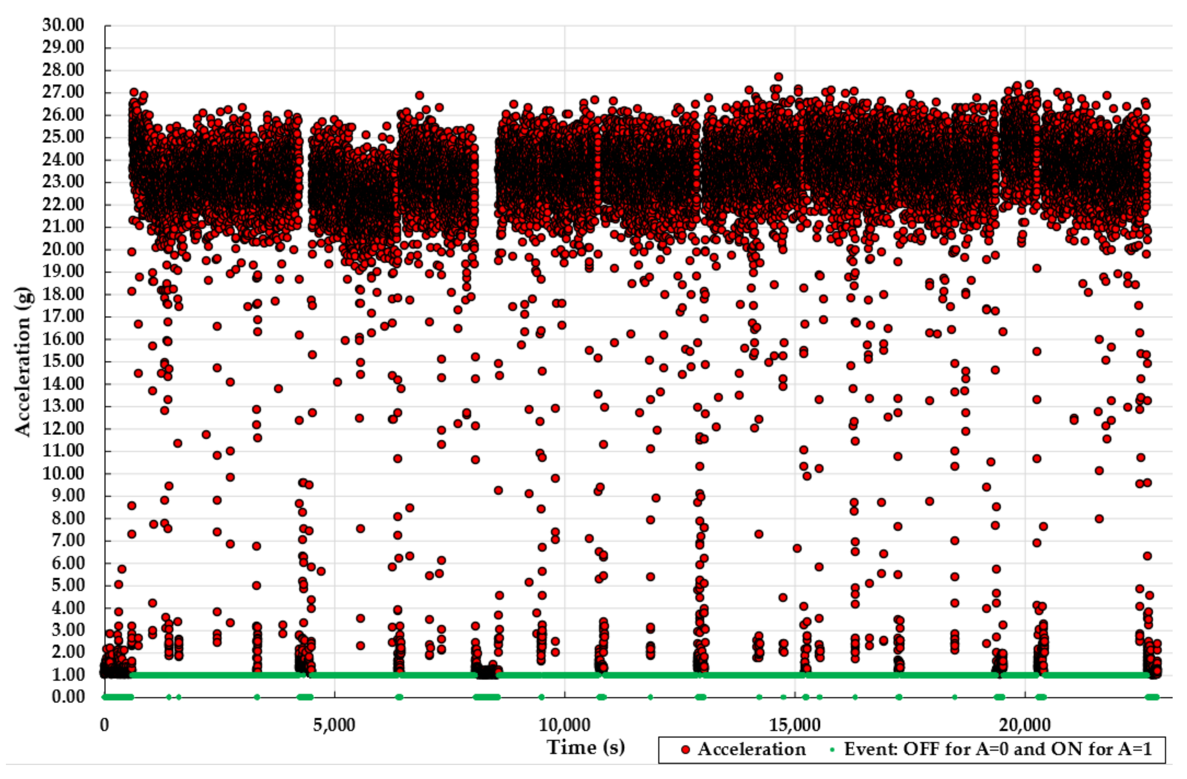
3.1. Description of the Labelled Datasets

The datasets used in this study accounted for a cumulated size of 107,276 s (ca. 30 h,

Table 2. Statistics of the used datasets.

Location	Dataset a	Size b [s]	Class Size [s]		Class Share [%]
			ON	OFF	ON	OFF
Poian 1	TRAIN_E	18,377	13,980	4487	76.07	23.93
	TRAIN_S	18,377	13,980	4487	76.07	23.93
	TRAIN	36,754	27,960	8794	76.07	23.93
Poian 2	TEST_E1	26,493	20,579	5914	77.68	22.32
	TEST_S1	22,885	20,404	2481	89.16	10.84
Belani	TEST_E2	11,859	6806	5053	57.39	42.61
	TEST_S2	9285	5886	3399	63.39	36.61
TOTAL	-	107,276 c	81,635 c	25,641 c	-	-

Note: ^a meaning is similar to that from Table 1; ^b size refers to the number of one-second sampled observations retained in the training and testing datasets; ^c calculated on the basis of the fused training dataset (TRAIN) and testing (TEST_E1, TEST_S1, TEST_E2, TEST_S2) datasets.

) of which the fused dataset used for training (TRAIN) represented ca. 34%. Datasets used for testing accounted (in their order shown in Table 2), for ca. 25%, 21%, 11% and 9%, respectively.

Excepting the dataset TEST_E2, data distribution on classes was found to preserve different degrees of class imbalance. Irrespective of the dataset, more than 57% of the data was labelled as ON, a class that accounted for ca. 90% of the TEST_S1 dataset’s size. While from the perspective of developing robust MLPs, this is a common issue to be solved [28], from an operational point of view this kind of data distributions emulates very well the practice of motor-manual willow felling, where the effective felling itself dominates.

3.2. Model Selection and Classification Performance

Values returned by the binary cross-entropy error as a function of the regularization parameter’s tunning are shown in Figure 3. Irrespective of the tunning strategy used, or the dataset in question, up to a value of α set at 1, the training and generalization errors were found to be less than 0.074 (7.4%, TEST_E2), showing, in general, a good generalization ability of the trained model. For values of α set from 0.0001 to 0.1, both the training (TRAIN) and generalization (TEST_E1, TEST_S1, TEST_E2, TEST_S2) errors were low, with the lowest ones found for α = 0.0001 and α = 0.1. Beyond this threshold (α = 0.1) the error started to noticeably increase at least for one of the testing datasets (Figure 3, TEST_E2). The lowest differences in terms of errors were found in the case of α = 0.0001 and α = 0.1 irrespective of the values compared (training and testing data or just testing data). For instance, when setting α at 0.0001, the value of the log loss in the case of training data was of 0.005 (0.5%) and it corresponded to a maximum value of 0.036 (3.6%) found in the TEST_E2 dataset. The figures were similar for α = 0.1, for which the error found for the training data was of 0.006 (0.6%), which corresponded to a maximum value of 0.037 (3.7%), found in the same testing dataset (TEST_E2). In term of errors, TRAIN and TEST_E1 datasets returned similar values for the range set for α between 0.0001 and 0.1. For the same range set for α, TEST_S1 and TEST_S2 datasets have returned a similar pattern in terms of errors.

Figure 4 is showing a comparison of the classification accuracy (CA) metric for the training and testing datasets, reflecting the effect that the value set for the α term had on this metric. In the training phase, all of the attempts to tune the regularization parameter term (α) returned very high classification accuracies. However, the classification accuracy of the training phase was preserved at the highest values (0.999, 99.9%) only in the range set for α between 0.0001 to 0.01, and it started to decrease as the regularization parameter approached the value set at 10. Moreover, the classification performance of the testing datasets was preserved to its highest values for α set in between 0.0001 and 0.01. However, the models selected for further assessment were those having this parameter set at 0.0001 and 0.1, based on the results returned by the log loss function, which are shown in Figure 3.

Table A1. Classification performance metrics of the training and testing datasets.

Regularization Parameter (Training Time)	Dataset	Area under Curve (AUC)	Classification Accuracy (CA)	F1	Precision (PREC)	Recall (REC)	Specificity (SPEC)
α = 0.0001 (261 s) a	TRAIN	1.000	0.999	0.999	0.999	0.999	0.997
	TEST_E1	1.000	0.999	0.999	0.999	0.999	0.996
	TEST_S1	1.000	0.996	0.996	0.996	0.996	0.989
	TEST_E2	0.999	0.994	0.994	0.994	0.994	0.995
	TEST_S2	0.999	0.991	0.991	0.991	0.991	0.986
α = 0.001 (326 s)	TRAIN	1.000	0.999	0.999	0.999	0.999	0.998
	TEST_E1	1.000	0.999	0.999	0.999	0.999	0.997
	TEST_S1	1.000	0.996	0.996	0.996	0.996	0.992
	TEST_E2	0.999	0.994	0.994	0.994	0.994	0.995
	TEST_S2	0.999	0.995	0.995	0.995	0.995	0.993
α = 0.01 (480 s)	TRAIN	1.000	0.999	0.999	0.999	0.999	0.998
	TEST_E1	1.000	0.999	0.999	0.999	0.999	0.997
	TEST_S1	1.000	0.996	0.996	0.996	0.996	0.992
	TEST_E2	0.999	0.994	0.994	0.994	0.994	0.995
	TEST_S2	0.999	0.995	0.995	0.995	0.995	0.994
α = 0.1 (443 s) a	TRAIN	1.000	0.998	0.998	0.998	0.998	0.998
	TEST_E1	1.000	0.999	0.999	0.999	0.999	0.998
	TEST_S1	1.000	0.995	0.995	0.995	0.995	0.992
	TEST_E2	0.999	0.994	0.994	0.994	0.994	0.995
	TEST_S2	0.999	0.995	0.995	0.995	0.995	0.994
α = 1 (482 s)	TRAIN	1.000	0.997	0.997	0.997	0.997	0.998
	TEST_E1	1.000	0.994	0.994	0.994	0.994	0.997
	TEST_S1	1.000	0.994	0.994	0.995	0.994	0.994
	TEST_E2	0.999	0.974	0.974	0.975	0.974	0.980
	TEST_S2	0.999	0.994	0.994	0.994	0.994	0.994
α = 10 (269 s)	TRAIN	1.000	0.994	0.994	0.994	0.994	0.998
	TEST_E1	1.000	0.990	0.990	0.991	0.990	0.996
	TEST_S1	1.000	0.994	0.994	0.994	0.994	0.995
	TEST_E2	0.999	0.944	0.944	0.950	0.944	0.958
	TEST_S2	0.999	0.993	0.993	0.993	0.993	0.995

Note: ^a regularization terms which returned the lowest log losses.

,

Table A2. Classification performance metrics of the training and testing datasets for ON events.

Regularization Parameter (Training Time)	Dataset	Area under Curve (AUC)	Classification Accuracy (CA)	F1	Precision (PREC)	Recall (REC)	Specificity (SPEC)
α = 0.0001 (261 s) a	TRAIN	1.000	0.999	0.999	0.999	0.999	0.997
	TEST_E1	1.000	0.999	0.999	0.998	1.000	0.994
	TEST_S1	1.000	0.996	0.998	0.999	0.997	0.988
	TEST_E2	0.999	0.994	0.995	0.997	0.992	0.996
	TEST_S2	0.999	0.991	0.993	0.988	0.998	0.979
α = 0.001 (326 s)	TRAIN	1.000	0.999	0.999	0.999	0.999	0.997
	TEST_E1	1.000	0.999	0.999	0.999	1.000	0.996
	TEST_S1	1.000	0.996	0.998	0.999	0.996	0.992
	TEST_E2	0.999	0.994	0.995	0.998	0.992	0.998
	TEST_S2	0.999	0.995	0.996	0.995	0.997	0.991
α = 0.01 (480 s)	TRAIN	1.000	0.999	0.999	0.999	0.999	0.997
	TEST_E1	1.000	0.999	0.999	0.999	1.000	0.996
	TEST_S1	1.000	0.996	0.997	0.999	0.996	0.992
	TEST_E2	0.999	0.994	0.995	0.998	0.992	0.998
	TEST_S2	0.999	0.995	0.996	0.995	0.996	0.992
α = 0.1 (443 s) a	TRAIN	1.000	0.998	0.999	0.999	0.998	0.997
	TEST_E1	1.000	0.999	0.999	0.999	1.000	0.997
	TEST_S1	1.000	0.995	0.997	0.999	0.996	0.992
	TEST_E2	0.999	0.994	0.995	0.999	0.991	0.998
	TEST_S2	0.999	0.995	0.996	0.996	0.996	0.994
α = 1 (482 s)	TRAIN	1.000	0.997	0.998	1.000	0.996	0.999
	TEST_E1	1.000	0.994	0.996	1.000	0.993	0.998
	TEST_S1	1.000	0.994	0.997	0.999	0.994	0.994
	TEST_E2	0.999	0.974	0.997	0.999	0.956	0.999
	TEST_S2	0.999	0.994	0.995	0.997	0.993	0.995
α = 10 (269 s)	TRAIN	1.000	0.994	0.996	1.000	0.993	0.999
	TEST_E1	1.000	0.990	0.994	1.000	0.988	0.999
	TEST_S1	1.000	0.994	0.997	0.999	0.994	0.996
	TEST_E2	0.999	0.944	0.948	0.999	0.903	0.999
	TEST_S2	0.999	0.993	0.995	0.998	0.992	0.996

Note: ^a regularization terms which returned the lowest log losses.

and

Table A3. Classification performance metrics of the training and testing datasets for OFF events.

Regularization Parameter (Training Time)	Dataset	Area under Curve (AUC)	Classification Accuracy (CA)	F1	Precision (PREC)	Recall (REC)	Specificity (SPEC)
α = 0.0001 (261 s) a	TRAIN	1.000	0.999	0.998	0.998	0.997	0.999
	TEST_E1	1.000	0.999	0.997	1.000	0.994	1.000
	TEST_S1	1.000	0.996	0.982	0.976	0.988	0.997
	TEST_E2	0.999	0.994	0.993	0.989	0.996	0.992
	TEST_S2	0.999	0.991	0.988	0.997	0.979	0.998
α = 0.001 (326 s)	TRAIN	1.000	0.999	0.997	0.997	0.997	0.999
	TEST_E1	1.000	0.999	0.998	1.000	0.996	1.000
	TEST_S1	1.000	0.996	0.980	0.970	0.992	0.996
	TEST_E2	0.999	0.994	0.993	0.989	0.998	0.992
	TEST_S2	0.999	0.995	0.993	0.995	0.991	0.997
α = 0.01 (480 s)	TRAIN	1.000	0.999	0.998	0.998	0.997	0.999
	TEST_E1	1.000	0.999	0.998	0.999	0.996	1.000
	TEST_S1	1.000	0.996	0.980	0.968	0.992	0.996
	TEST_E2	0.999	0.994	0.993	0.989	0.998	0.992
	TEST_S2	0.999	0.995	0.993	0.994	0.992	0.996
α = 0.1 (443 s) a	TRAIN	1.000	0.998	0.996	0.995	0.997	0.998
	TEST_E1	1.000	0.999	0.998	0.999	0.997	1.000
	TEST_S1	1.000	0.995	0.979	0.965	0.992	0.996
	TEST_E2	0.999	0.994	0.993	0.988	0.998	0.991
	TEST_S2	0.999	0.995	0.993	0.993	0.994	0.996
α = 1 (482 s)	TRAIN	1.000	0.997	0.994	0.989	0.999	0.996
	TEST_E1	1.000	0.994	0.987	0.976	0.998	0.993
	TEST_S1	1.000	0.994	0.974	0.955	0.994	0.994
	TEST_E2	0.999	0.974	0.970	0.944	0.999	0.956
	TEST_S2	0.999	0.994	0.992	0.988	0.995	0.993
α = 10 (269 s)	TRAIN	1.000	0.994	0.988	0.977	0.999	0.993
	TEST_E1	1.000	0.990	0.979	0.960	0.999	0.988
	TEST_S1	1.000	0.994	0.974	0.953	0.996	0.994
	TEST_E2	0.999	0.944	0.938	0.884	0.999	0.903
	TEST_S2	0.999	0.993	0.991	0.986	0.996	0.992

Note: ^a regularization terms which returned the lowest log losses.

are showing the detailed classification performance metrics at the overall (dataset) level, as well as on classes (ON, OFF). Irrespective of the class, the minimum values of classification accuracy (CA) metric were of 0.944 (94%), indicating a high share of correct predictions for the worst prediction case. The minimum values of the F1 metric, which stands for the harmonic mean of precision (PREC) and recall (REC), were of 0.944 (94%), 0.948 (95%) and 0.938 (94%) for the overall, ON and OFF data. In the same order, the minimum values of classification precision (PREC) and recall (REC) were of 0.950 (95%), 0.988 (99%), 0.884 (88%) and of 0.903 (90%), 0.903 (90%) and 0.988 (99%), respectively, where precision stands for the fraction of true positives from the total of positives (TP and FP) and recall stands for the fraction of correctly classified true positives from the total positives. Accordingly, these metrics returned high values for the worst prediction cases, with evident differences as a result of the regularization parameter tunning. Training time of the MLP varied in between ca. 261 and 482 s, and it was of ca. 261 and 443 s for the models trained for α = 0.0001 and 0.1, respectively. A more detailed comparison of the classification accuracy for the former models is given in

Table 3. Classification accuracy of the selected models.

Class	TRAIN		TEST_E1		TEST_S1		TEST_E2		TEST_S2
	α = 0.0001	α = 0.1	α = 0.0001	α = 0.1	α = 0.0001	α = 0.1	α = 0.0001	α = 0.1	α = 0.0001	α = 0.1
ON	0.999	0.998	0.999	0.999	0.996	0.995	0.994	0.994	0.991	0.995
OFF	0.999	0.998	0.999	0.999	0.996	0.995	0.994	0.994	0.991	0.995
OVERALL	0.999	0.998	0.999	0.999	0.996	0.995	0.994	0.994	0.991	0.995

, showing some of the highest values of the CA among the set of regularization terms used.

Excepting the TEST_S2 dataset, no significant differences were found in terms of classification accuracy as an effect of tuning the regularization parameter. In addition, classification performance was found to be very high in the case of most of the testing datasets, and in terms of classification accuracy (CA), its values ranged from 99.1% (TEST_S2, α = 0.0001) to 99.9% (TEST_E1), proving a high generalization ability of the trained models.

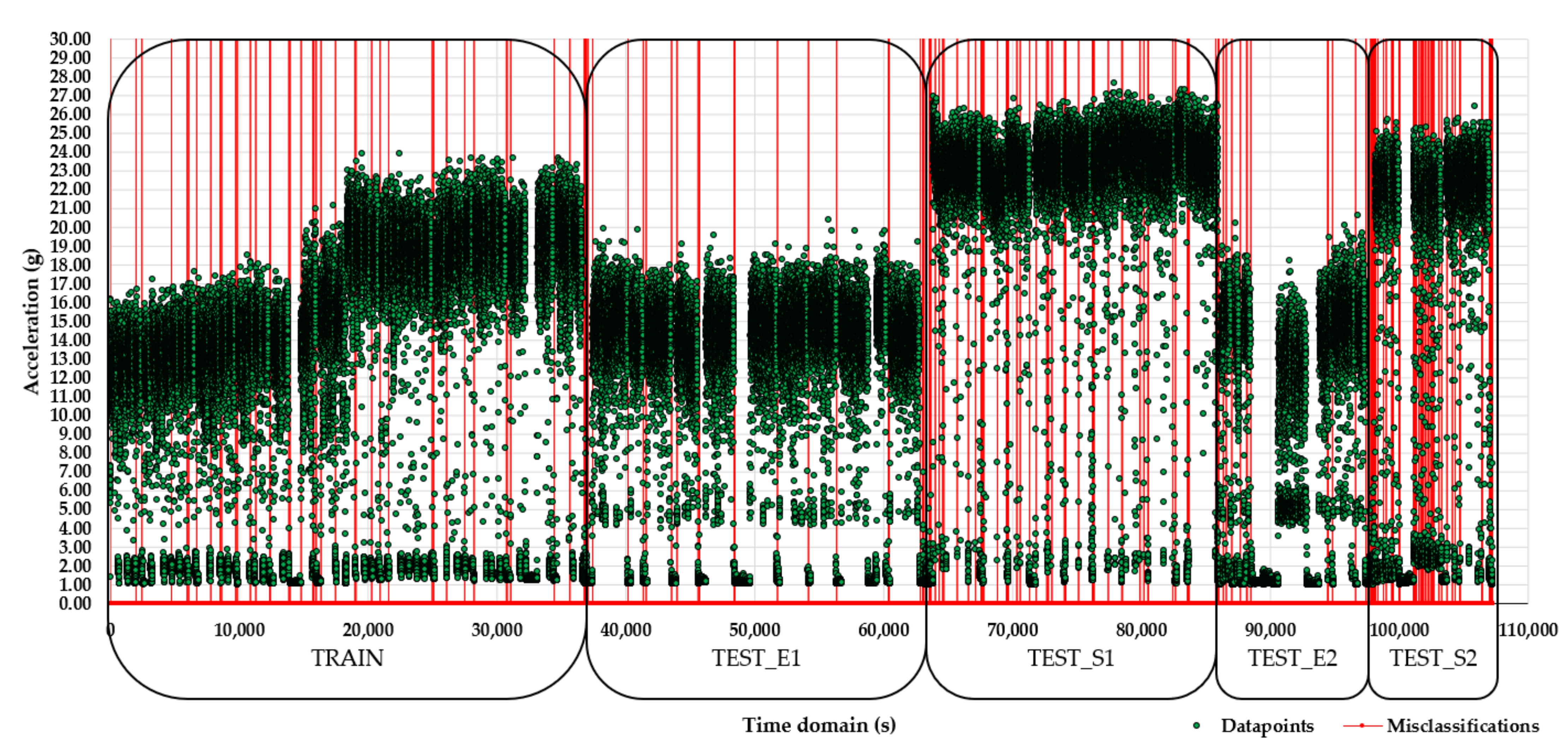
3.3. Missclassification and Probability Plots

The correctly classified observations in the training dataset (TRAIN,

Table 4. Descriptive statistics of misclassifications.

Regularization Term	Dataset a	Size b [s]	Correctly Classified		Misclassified as
					False Positives		False Negatives
			N	Share (%)	N	Share (%)	N	Share (%)
α = 0.0001	TRAIN	36,754	36,711	99.88	28	0.08	15	0.04
	TEST_E1	26,493	26,465	99.89	2	0.01	26	0.10
	TEST_S1	22,885	22,795	99.61	40	0.18	50	0.22
	TEST_E2	11,859	11,788	99.40	15	0.13	56	0.47
	TEST_S2	9285	9202	99.11	73	0.78	10	0.11
	TOTAL	107,276	-	-	-	-	-	-
α = 0.1	TRAIN	36,754	36,686	99.82	23	0.06	45	0.12
	TEST_E1	26,493	26,469	99.90	12	0.05	12	0.05
	TEST_S1	22,885	22,787	99.57	21	0.09	77	0.34
	TEST_E2	11,859	11,784	99.37	8	0.07	67	0.56
	TEST_S2	9285	9237	99.48	26	0.28	22	0.24
	TOTAL	107,276	-	-	-	-	-	-

Note: ^a meaning is similar to that from Table 1; ^b size refers to the number of one-second sampled observations retained in the training and testing datasets.

) were close in terms of relative frequency. In absolute numbers, however, the model using a regularization term set at 0.1 misclassified more (25 observations) compared to that of α set at 0.0001. When checked for the testing datasets (TEST_E1, TEST_S1, TEST_E2, Table 4), the number of misclassifications was relatively tied in relation to the regularization parameter term used, excepting the last testing dataset (TEST_S2, Table 4) which returned a better performance for α set at 0.1. Figure 5 is giving a representation of misclassified data points in the training and testing datasets for a regularization parameter term set at 0.0001. Irrespective of the dataset, the misclassified datapoints shared a common feature, namely their location in terms of magnitude in the transient data segments characterizing inter-class variability. These segments were those mostly identified for operational events such as turning on or off the tool’s engine, and which were formally included in the ON class. However, no attempts were taken to separate another class given the results obtained on classification performance and error metrics (Figure 3 and Figure 4, Table 3 and Table 4), which were considered to be acceptable. In addition, the number of observations which were found to be misclassified due to their belonging to these events is typically low in applications such as that studied herein (Table 4).

Figure 6 is showing a selection of predicted probability plots in a comparative approach. The data shown stands for the dataset used for training (TRAIN), as well as for datasets TEST_E2 and TEST_S1 used for testing. It compares the predicted probabilities of the datapoints from the abovementioned datasets of belonging to the classes ON and OFF, respectively, against the values of those datapoints computed according to the Equation (1).

For a value of the regularization parameter term set at 0.0001, the minimum values of the Euclidian Norm found to be predicted as ON were close to 3 g in all the datasets (detailed statistics are not shown herein, and Figure 6 shows only a selection of predicted probability plots). Accordingly, the maximum values of the Euclidian Norm found to be predicted as OFF were close to 3 g in most of the datasets. In comparison, for a value of the regularization parameter term set at 0.1, the minimum and maximum threshold values (as described above) of the Euclidian Norm were close to 4 g in most of the datasets. These statistics can be followed quite easy in Figure 6, where in the left panels (α = 0.0001) the predicted probability data is split for a probability set at 0.5 by a value close to 3. Accordingly, the left panels of the figure (α = 0. 1) split the predicted probability data, at the same probability threshold (0.5), by a value of the Euclidian Norm close to 4 g.

4. Discussion

Monitoring the operational performance is one of the common ways to get the data needed for sound decisions on running and improving the way that various businesses work. It is already a fact that many manufacturing industries are currently collecting sensor-based data to improve their operations and to respond by informed decisions to various production anomalies and problems [41], enabling them to be more competitive, responsive and resilient. In forest and SRWC operations, getting monitoring data was traditionally based on observing workers, tools and machines by time-and-motion studies [12,13,14], which have evolved from pen-and-paper to various sensing-based techniques; the latter are often implementing an external rather than a built-in sensor system e.g., [7,10,15,17,18,20,23,42,43,44,45,46] mainly due to their purpose for collecting such data, which was often purely scientific. Although the modern machines may incorporate production monitoring systems that may work in real time, there are still few options to collect and handle such data for hand-operated tools. Recent studies have shown that the acceleration sensors may be successfully used to collect long term operational monitoring data e.g., [7,10,16,17,23,43,45,47] including by the use of platforms such as the smartphones [15]. In many cases, however, such data comes as modality-variant, unannotated sets, requiring significant resources to process and analyze it [7,10,47]. In this regard, the merit of this study is that it developed data collection invariant models able to automatically and accurately classify, analyze and interpret signals collected by triaxial accelerometers, enabling the possibility to extend their applicability to new coming datasets. As such, the implementation of MLP can serve to automatically classify new data recorded by triaxial accelerometers, irrespective of the datalogger placement on the tool.

One of the relevant issues for discussion is the sensing modality itself. Dealing with sensing modalities is not a new approach brought by this paper as it has been discussed [28] and used by other studies making use of sensors to measure various physical variables [15,17,30,47,48]. However, as there is no certainty that in follow-up field data collection activities the acceleration dataloggers will be placed at the same location each time, the developed models need to produce classifications that are invariant to such issues. By fusing the Euclidian Norm data collected on two of the most accessible parts of the tool, this study has facilitated the attempt of making the models invariant to the data sensing location. This is proven by the results obtained on the testing datasets, which returned in all the cases excellent classification results (Table A1, Table A2 and Table A3), irrespective of the datalogger placement, operational variability or the individual handling of the tool. Moreover, the developed models were found to deal very well with the intra-class variability of the Euclidian Norm data (Figure 3, events labelled with 2 and 3 for a single sensing modality: engine (TRAIN_E) or transmission shaft (TRAIN_S)), which was mostly generated by the variation of operational behavior. As a fact, intra-class variability may be related to and generated by the same or more individuals performing differently something in a given activity [49]. In this study, intra-class variability was the effect of operational behavior in relation to the crop layout, some portions requiring walking with engine in the idle running, as well as the effect of other issues such as changes in the operational behavior for similar operational conditions. For a comparison, the reader may consult, for instance, Figure A2 and Figure A4. However, a speculation that could be raised here is that the use of vibration data sensed by a direct contact with the tool has more potential in generating more clearly separable events; hence, it could stand for a good approach to eliminate much of the intra-class variability which could be generated by different persons carrying on the same task. Due to the vibration characteristics of the tools equipped with two-stroke engines, the models developed and tested in this study might work well also on data collected by sensor placement on the chainsaws to distinguish between engine working (ON) and non-working states (OFF). For instance, the work of [16] has shown a similar data pattern and vibration magnitudes for engine working states. However, further studies are needed to check if the models would work on tools from other classes that are characterized by contrasting constructive concepts.

Class imbalance [28,49] and inter-class similarity [49] are common issues causing classification problems in various applications of the human activity recognition. On the one hand, class imbalance biases the prediction of conventional models toward the classes holding the majority of data [28]. On the other hand, experiments that are purely observational hold few if no ways to address this challenge [12,14], as the occurrence of the datapoints in given classes is imposed by the operational conditions. Class imbalance was a defining feature of the datasets used in this study, which have shown a data majority attributed to the ON class (Table 2). Given the results of classification performance, however, it seems that this characteristic had small effects on the datasets if compared, for instance, to inter-class similarity (transient events such as turning on and of the engine), which resulted in some misclassifications (Table 4, Figure 5 and Figure 6).

Classification performance of the models was found to be very high, while keeping the error rates at a low level in both the training and testing datasets. For instance, classification accuracy was higher than 99% irrespective of the explored dataset, a value that is frequently termed as being very good [40]. However, there was a tradeoff between achieving high classification performances and keeping the generalization errors low, which in this study was evaluated by a trial-and-error approach which tuned the regularization parameter and lead to a selection of two final best-performing models. The final models (for α set at 0.0001 and 0.1, respectively), which were retained based on their lowest generalization errors, shared similar classification accuracies, excepting that of the TEST_S2 dataset, a case in which the model trained for α = 0.1 performed better. Given the similarity of classification accuracy for the rest of comparisons (Table 3), this outcome could be attributed to the functions and decision boundaries learned by the MLP model.

In addition to the hyperparameters’ tuning, classification performance is affected by the architecture of the MLP (particularly the size) but also by the sensing modalities. Most often, the size of the MLP is selected based on rules of thumb [50,51]. However, the work of [16] has shown how an increasing depth (number of hidden layers) and width (number of neurons in a hidden layer) of the MLP may output increasingly accurate classification results for a case study run on triaxial acceleration data collected on a chainsaw. Based on that, as well as on the recommendations of [33], the size of the MLP was set to the maximum allowed by the used software. Sensing by two or more modalities may increase the classification performance. For instance, the work of [15] has found that the use of sound in addition to acceleration and gyroscope-collected data contributed to the performance increment of a Random Forest algorithm by decreasing the classification errors, while the work of [17] has found a better classification performance when fusing the data on acceleration and sound pressure level by horizontal staking before feeding it into MLPs, concluding that the preservation of sensing location may be of high importance in developing more accurate classification models. By comparison, this study removes the problem of sensing location by training the MLPs on dual-sensed signals collected at two locations on the tool. While further studies would be needed to check it, by its specific learning characteristics, the developed MLP could be invariant to the sampling rate of new coming data, because it makes its predictions based on the functions learned and not based on the sampling rate characteristics.

Collecting, processing, analyzing and interpreting large amounts of data is one of the approaches taken today to better understand ecological, social and technical systems, enabling a better decision making based on deeply informed grounds. There are several approaches, techniques and technologies to the problem which have already been described as being opportune for the general forestry [52]. Operational monitoring of SRWCs may benefit from sensor-based data collection approaches coupled with the techniques of artificial intelligence by removing the human error and the effort associated to the traditional observation [53,54]. Moreover, approaches such that described in this study could be used to prevent the safety issues associated with collecting data near dangerous machines and tools or in difficult outdoor conditions [12], being also less intrusive in applications that aim at observing people at work. At the time of purchasing the dataloggers used in this study, they were considered to be very small and useful for operational monitoring of motor-manual operations [47,48]. However, the technology of producing affordable miniaturized sensors in ongoing and had a significant progress, since smaller sensors are already released on the market, facilitating the transition to sensor-based operational monitoring. This progress has been reflected positively in various forestry applications requiring close-range sensing [55], and there is a lot of unexplored potential for such techniques both in forest and in WSRC operations.

There are two main limitations of this study. The first one is related to the MLP’s misclassifications which were mainly found for those datapoints characterizing the so-called transient events of turning on and off the tool’s engine (Table 4, Figure 5). The second one is related to the fact that in this study the data was segmented only in two classes, therefore the engine idle time was included in the same class as the effective willow felling time. Both of these problems may be easily solved by adding more context by the use of GPS units, an approach that has shown good results in previous studies on the topic [7,10]. In addition, in the phase of data interpretation, one can treat misclassifications as non-felling time having in mind the knowledge gained by this study. However, further studies are needed to evaluate whether adding primary and derived GPS location data into the MLP would help in designing applications able to look more deeply into the underlying process of willow felling operations. For instance, GPS coordinates and speed were used to infer the location and operational behavior of a feller by a traditional human-assisted classification approach [7,10] and they could provide additional context for the design of a multiclass MLP.

5. Conclusions

For a binary classification problem which emulates the most important operational events in SRWCs’ motor-manual felling by brush cutters, the developed MLPs have returned high classification accuracies (99.1% to 99.9%) which were invariant to the sensing modality judged by the sensors’ location. While the study has addressed hyperparameter tunning by the modification of the regularization parameter term, two final models were retained as being able to (i) provide high classification accuracies, (ii) generalize well on the testing datasets collected by single modalities and (iii) retain low errors in both, the training and testing phases. Given the obtained results, the developed models are assumed to be invariant to the new coming data, making them useful in classification applications and enabling the automation of most of the workflow typically implemented to collect, process, analyze and interpret large amounts of data. Further studies could bring new interesting and valuable insights if focused on evaluating the classification performance by the possibility of adding more context to the developed MLPs. This could be achieved by fusing the triaxial acceleration data with that collected by miniaturized GPS units to be able to classify and describe in more depth the operational tasks.

References

1. Dickmann, D.I. Silviculture and biology of short-rotation woody crops in temperate regions: Then and now. Biomass Bioenerg. 2006, 30, 696–705. [Google Scholar] [CrossRef]
2. Kuzovkina, Y.A.; Volk, T.A. The characterization of willow (Salix L.) varieties for use in ecological engineering applications: Co-ordination of structure, function and autecology. Ecol. Eng. 2009, 35, 1178–1189. [Google Scholar] [CrossRef]
3. Berhongaray, G.; El Kasmioui, O.; Ceulemans, R. Comparative analysis of harvesting machines on operational high-density short rotation woody crop (SRWC) culture: One-process versus two-process harvest operation. Biomass Bioenerg. 2013, 58, 333–342. [Google Scholar] [CrossRef] [Green Version]
4. Schweier, J.; Becker, G. Harvesting of short rotation coppice—Harvesting trials with a cut and storage system in Germany. Silva Fenn. 2012, 46, 287–299. [Google Scholar] [CrossRef] [Green Version]
5. El Kasmioui, O.; Ceulemans, R. Financial analysis of the cultivation of short rotation woody crops for bioenergy in Belgium: Barriers and opportunities. Bioenerg. Res. 2013, 6, 336–350. [Google Scholar] [CrossRef]
6. Buchholz, T.; Volk, T.A. Improving the profitability of willow crops—Identifying opportunities with a crop budget model. Bioenerg. Res. 2011, 4, 85–95. [Google Scholar] [CrossRef]
7. Borz, S.A.; Talagai, N.; Cheţa, M.; Chiriloiu, D.; Gavilanes Montoya, A.V.; Castillo Vizuete, D.D.; Marcu, M.V. Physical strain, exposure to noise and postural assessment in motor-manual felling of willow short rotation coppice: Results of a preliminary study. Croat. J. Eng. 2019, 40, 377–388. [Google Scholar] [CrossRef]
8. Schweier, J.; Becker, G. Motor manual harvest of short rotation coppice in South-West Germany. Allg. Forst-und Jagdztg. 2012, 183, 159–167. [Google Scholar]
9. Talagai, N.; Borz, S.A.; Ignea, G. Performance of brush cutters in felling operations of willow short rotation coppice. Bioresources 2017, 12, 3560–3569. [Google Scholar] [CrossRef]
10. Borz, S.A.; Talagai, N.; Cheţa, M.; Gavilanes Montoya, A.V.; Castillo Vizuete, D.D. Automating data collection in motor-manual time and motion studies implemented in a willow short rotation coppice. Bioresources 2018, 13, 3236–3249. [Google Scholar] [CrossRef]
11. Vanbeveren, S.P.P.; Schweier, J.; Berhongaray, G.; Ceulemans, R. Operational short rotation woody crops plantations: Manual or mechanized harvesting? Biomass Bioenerg. 2015, 72, 8–18. [Google Scholar] [CrossRef]
12. Acuna, M.; Bigot, M.; Guerra, S.; Hartsough, B.; Kanzian, C.; Kärhä, K.; Lindroos, O.; Magagnotti, N.; Roux, S.; Spinelli, R.; et al. Good Practice Guidelines for Biomass Production Studies; Magagnotti, N., Spinelli, R., Eds.; CNR IVALSA: Sesto Fiorentino, Italy, 2012; Available online: http://www.forestenergy.org/pages/cost-action-fp0902/good-practice-guidelines/ (accessed on 15 April 2018).
13. Björheden, R.; Apel, K.; Shiba, M.; Thompson, M. IUFRO Forest Work Study Nomenclature; Swedish University of Agricultural Science, Department of Operational Efficiency: Grapenberg, Sweden, 1995. [Google Scholar]
14. Borz, S.A. Evaluarea Eficienţei Echipamentelor şi Sistemelor Tehnice în Operaţii Forestiere; Lux Libris Publishing House: Braşov, Romania, 2008. [Google Scholar]
15. Keefe, R.F.; Zimbelman, E.G.; Wempe, A.M. Use of smartphone sensors to quantify the productive cycle elements of hand fallers on industrial cable logging operations. Int. J. Eng. 2019, 30, 132–143. [Google Scholar] [CrossRef]
16. Cheţa, M.; Marcu, M.V.; Borz, S.A. Effect of training parameters on the ability of artificial neural networks to learn: A simulation on accelerometer data for task recognition in motor-manual felling and processing. Bull. Transilv. Univ. Bras. Ser. Wood Ind. Agric. Food Eng. 2020, 131, 19–36. [Google Scholar] [CrossRef]
17. Cheţa, M.; Marcu, M.V.; Iordache, E.; Borz, S.A. Testing the capability of low-cost tools and artificial intelligence techniques to automatically detect operations done by a small-sized manually driven bandsaw. Forests 2020, 11, 739. [Google Scholar] [CrossRef]
18. Borz, S.A.; Păun, M. Integrating offline object tracking, signal processing and artificial intelligence to classify relevant events in sawmilling operations. Forests 2020, 11, 1333. [Google Scholar] [CrossRef]
19. Talagai, N.; Borz, S.A. Concepte de automatizare a activităţii de colectare a datelor cu aplicabilitate în monitorizarea performanţei productive în operaţii de gestionare a culturilor de salcie rotaţie scurtă. Rev. Pădurilor 2016, 131, 78–94. [Google Scholar]
20. Talagai, N.; Marcu, M.V.; Zimbalatti, G.; Proto, A.R.; Borz, S.A. Productivity in partly mechanized planting operations of willow short rotation coppice. Biomass Bioenerg. 2020, 138, 105–609. [Google Scholar] [CrossRef]
21. Borz, S.A.; Niţa, M.D.; Talagai, N.; Scriba, C.; Grigolato, S.; Proto, A.R. Performance of small-scale technology in planting and cutback operations of short-rotation willow crops. Trans. ASABE 2019, 62, 167–176. [Google Scholar] [CrossRef]
22. User Guide of the Husqvarna 545 Series (In Romanian). Available online: https://www.husqvarna.com/ro/products/motounelte-motocoase/545rx/966015901/ (accessed on 16 February 2021).
23. Talagai, N.; Cheţa, M.; Gavilanes Montoya, A.V.; Castillo Vizuete, D.D.; Borz, S.A. Predicting time consumption of chipping tasks in a willow short rotation coppice from GPS and acceleration data. In Proceedings of the Biennial International Symposium “Forest and Sustainable Development”, Braşov, Romania, 25–27 October 2018; Borz, S.A., Curtu, A.L., Muşat, E.C., Eds.; Transilvania University Press: Braşov, Romania, 2019; pp. 1–12. [Google Scholar]
24. Boja, N.; Borz, S.A. Energy inputs in motor-manual release cutting of broadleaved forests: Results of twelve options. Energies 2020, 13, 4597. [Google Scholar] [CrossRef]
25. Ignea, G.; Ghaffaryian, M.R.; Borz, S.A. Impact of operational factors on fossil energy inputs in motor-manual tree felling and processing operations: Results of two case studies. Ann. Res. 2017, 60, 161–172. [Google Scholar] [CrossRef] [Green Version]
26. Technical Specifications of the Extech® VB300 3-Axis G-force USB Datalogger. Available online: http://www.extech.com/products/VB300 (accessed on 17 February 2021).
27. Technical specifications of the Extech® 407760 USB Sound Level Datalogger. Available online: http://www.extech.com/products/407760 (accessed on 17 February 2021).
28. Chen, K.; Zhang, D.; Yao, L.; Guo, B.; Yu, Z.; Liu, Y. Deep learning for sensor-based human activity recognition: Overview, challenges and opportunities. J. ACM 2018, 37, 111. [Google Scholar]
29. Van Hees, V.T.; Gorzelniak, L.; Dean Leon, E.C.; Eder, M.; Pias, M.; Taherian, S.; Ekelund, U.; Renström, F.; Franks, P.W.; Horsch, A.; et al. Separating movement and gravity components in acceleration signal and implications for the assessment of human daily physical activity. PLoS ONE 2013, 8, e61691. [Google Scholar] [CrossRef] [PubMed] [Green Version]
30. Ha, S.; Yun, J.-M.; Chi, S. Multi-modal convolutional neural networks for activity recognition. In Proceedings of the 2015 IEEE Conference on Systems, Man and Cybernetics, Hong Kong, China, 9–12 October 2015; pp. 3017–3022. [Google Scholar] [CrossRef]
31. Han, J.; Kamber, M.; Pei, J. Data Mining: Concepts and Techniques, 3rd ed.; Morgan Kaufmann Publishers: Burlington, MA, USA, 2006. [Google Scholar]
32. Demsar, J.; Curk, T.; Erjavec, A.; Gorup, C.; Hocevar, T.; Milutinovic, M.; Mozina, M.; Polajnar, M.; Toplak, M.; Staric, A.; et al. Orange: Data Mining Toolbox in Python. J. Mach. Learn. Res. 2013, 14, 2349–2353. [Google Scholar]
33. Goodfellow, J.; Bengio, Y.; Courville, A. Deep Learning; MIT Press: Cambridge, MA, USA, 2016; Available online: https://www.deeplearningbook.org/ (accessed on 17 February 2021).
34. Maas, A.L.; Hannun, A.Y.; Ng, A.Y. Rectifier nonlinearities improve neural network acoustic models. In Proceedings of the 30th International Conference on Machine Learning, ICML 2013, Atlanta, GA, USA, 16–21 June 2013. [Google Scholar]
35. Nair, V.; Hinton, G.E. Rectified linear units improve restricted Boltzmann machines. In Proceedings of the 27th International Conference on Machine Learning (ICML 2010), Haifa, Israel, 21–24 June 2010. [Google Scholar]
36. Kingma, D.P.; Ba, J.L. ADAM: A method for stochastic optimization. In Proceedings of the 3rd International Conference on Learning Representations, ICLR 2015, San Diego, CA, USA, 7–9 May 2015. [Google Scholar]
37. Varying Regularization in Multi-Layer Perceptrons. Available online: https://scikit-learn.org/stable/auto_examples/neural_networks/plot_mlp_alpha.html#sphx-glr-auto-examples-neural-networks-plot-mlp-alpha-py (accessed on 17 February 2021).
38. Understanding Binary Cross-Entropy/Log-Loss: A Visual Explanation. By Daniel Godoy. Available online: https://towardsdatascience.com/understanding-binary-cross-entropy-log-loss-a-visual-explanation-a3ac6025181a (accessed on 17 February 2021).
39. Fawcett, T. An introduction to ROC analysis. Pattern Recogn. Lett. 2006, 27, 861–874. [Google Scholar] [CrossRef]
40. Kamilaris, A.; Prenafeta-Boldu, F.X. Deep learning in agriculture: A survey. Comput. Electron. Agric. 2018, 147, 70–90. [Google Scholar] [CrossRef] [Green Version]
41. Wescoat, E.; Krugh, M.; Henderson, A.; Goodnough, J.; Mears, L. Vibration analysis using unsupervised learning. Procedia Manuf. 2019, 34, 876–884. [Google Scholar] [CrossRef]
42. McDonald, T.P.; Fulton, J.P. Automated time study of skidders using global positioning system data. Comput. Electron. Agric. 2005, 48, 19–37. [Google Scholar] [CrossRef] [Green Version]
43. Strandgard, M.; Mitchell, R. Automated time study of forwarders using GPS and a vibration sensor. Croat. J. Eng. 2015, 36, 175–184. [Google Scholar]
44. Contreras, M.; Freitas, R.; Ribeiro, L.; Stringer, J.; Clark, C. Multi-camera surveillance systems for time and motion studies of timber harvesting equipment. Comput. Electron. Agric. 2015, 135, 208–215. [Google Scholar] [CrossRef]
45. McDonald, T.P.; Fulton, J.P.; Darr, M.J.; Gallagher, T.V. Evaluation of a system to spatially monitor hand planting of pine seedlings. Comput. Electron. Agric. 2008, 64, 173–182. [Google Scholar] [CrossRef]
46. Borz, S.A.; Marcu, M.V.; Cataldo, M.F. Evaluation of a HSM 208F 14tone HVT-R2 forwarder prototype under conditions of steep-terrain low-access forests. Croat. J. For. Eng. [CrossRef]
47. Marogel-Popa, T.; Cheţa, M.; Marcu, M.V.; Duţă, I.; Ioraș, F.; Borz, S.A. Manual cultivation operations in poplar stands: A characterization of job difficulty and risks of health impairment. Int. J. Env. Res. Public Health 2019, 16, 1911. [Google Scholar] [CrossRef] [Green Version]
48. Cheţa, M.; Marcu, M.V.; Borz, S.A. Workload, exposure to noise, and risk of musculoskeletal disorders: A case study of motor-manual tree felling and processing in poplar clear cuts. Forests 2018, 9, 300. [Google Scholar] [CrossRef] [Green Version]
49. Bulling, A.; Blanke, U.; Schiele, B. A tutorial of human activity recognition using body-worn inertial sensors. ACM Comput. Surv. 2014, 46, 33. [Google Scholar] [CrossRef]
50. Karsoliya, S. Approximating number of hidden layer neurons in multiple hidden layer BPNN architecture. Int. J. Eng. Technol. 2012, 3, 714–717. [Google Scholar]
51. Panchal, F.S.; Panchal, M. Review on methods of selecting number of hidden nodes in Artificial Neural Network. Int. J. Comput. Sci. Mob. Comput. 2014, 3, 455–464. [Google Scholar]
52. Keefe, R.F.; Wempe, A.M.; Becker, R.M.; Zimbelman, E.G.; Nagler, E.S.; Gilbert, S.L.; Caudill, C.C. Positioning methods and the use of location and activity data in forests. Forests 2019, 10, 458. [Google Scholar] [CrossRef] [Green Version]
53. Borz, S.A. Turning a winch skidder into a self-data collection machine. Bull. Transilv. Univ. Bras. Ser. Wood Ind. Agric. Food Eng. 2016, 9, 1–6. [Google Scholar]
54. Spinelli, R.; Laina-Relano, R.; Magagnotti, N.; Tolosana, E. Determining observer effect and method effects on the accuracy of elemental time studies in forest operations. Balt. For. 2013, 19, 301–306. [Google Scholar]
55. Picchio, R.; Proto, A.R.; Civitarese, V.; Di Marzio, N.; Latterini, F. Recent contributions of some fields of the electronics in development of forest operations technologies. Electronics 2019, 8, 1465. [Google Scholar] [CrossRef] [Green Version]
Figure 1. Work organization, tool description and instrumentation of data collection. Legend: (a)—the typical work organization (1—bunch of stems to be felled, 2—bunches of felled stems, 3—wooden stick used to direct the felling, 4—throttling control, 5—engine, 6—transmission shaft, 7—steel blade, 8—triaxial accelerometer, 9—helmet equipped with a sound pressure level datalogger), (b)—the general layout of the felling operations (example from Poian 1 location, close to finishing the felling work in a plot), (c)—detail of the acceleration datalogger (8) placed on the shaft, (d)—details on the instrumentation used to collect the data (8—triaxial accelerometers, 9—sound pressure level datalogger).
Forests 12 00406 g001
Figure 2. A sample from the acceleration and sound pressure level datasets used jointly to label the data. Note: for convenience, the sound pressure level data was downscaled by a factor of 100 to help in data comparison and labelling tasks. Legend: TRAIN_E stands for the training dataset collected by the placement of acceleration datalogger on the tool’s engine, TRAIN_S stands for the training dataset collected by the placement of acceleration datalogger on the tool’s transmission shaft, LABELLING stands for the sound pressure level data downscaled by a factor of 100; Events: 1—engine off and no movement of the worker (labelled as OFF), 2—engine on and felling (labelled as ON), 3—engine on and not felling (labelled as ON), 4—engine off and movement of the worker (labelled OFF), 5—data segments which were transient (inter-class variability) between the two engine states (labelled as ON).
Forests 12 00406 g002
Figure 3. Log loss (binary cross-entropy) of the training and testing data as a function of the regularization parameter term (α). Legend: TRAIN—fused training dataset, TEST_E1 and TEST_E2—testing datasets collected on the tool’s engine, TEST_S1 and TEST_S2—testing datasets collected on the tools’ transmission shaft. Note: Values shown are computed by using Equation (3), based on the normalized data (Equation (2)); models retained for further analysis are bordered by green dashed lines.
Forests 12 00406 g003
Figure 4. Classification accuracy scored at the training (TRAIN) and testing (TEST_E1, TEST_S1, TEST_E2, TEST_S2) phases, as a function of the value of the regularization parameter (α).
Forests 12 00406 g004
Figure 5. Distribution of misclassifications in the training (TRAIN) and testing (TEST_E1, TEST_S1, TEST_E2, TEST_S2) datasets for a regularization term (α) set at 0.0001. Legend: green points stand for the Euclidian Norm (EN); red lines stand for correctly classified datapoints when drawn horizontally at an EN of 0, and for misclassified datapoints when drawn vertically. Note: for convenience the datasets were merged in their order of analysis.
Forests 12 00406 g005
Figure 6. Selected plots showing the predicted classification probability. Legend: P(OFF), shown in red, stands for the predicted probabilities of the datapoints being OFF and P(ON), shown in green, stands for the predicted probabilities of the datapoints being ON. Note: (a,b)—predicted classification probability for the TRAIN dataset; (c,d)—predicted classification probability for the TEST_E2 dataset; (e,f)—predicted classification probability for the TEST_S1 dataset; left figure panels show the data for α = 0.0001 and the right figure panels show the data for α = 0.1.
Forests 12 00406 g006aForests 12 00406 g006b