Disentangling the Ecological Determinants of Species and Functional Trait Diversity in Herb-Layer Plant Communities in European Temperate Forests

Abstract

Forest herb-layer vegetation responds sensitively to environmental conditions. This paper compares drivers of both taxonomic, i.e., species richness, cover and evenness, and functional herb-layer diversity, i.e., the diversity of clonal, bud bank and leaf-height-seed plant traits. We investigated the dependence of herb-layer diversity on ecological determinants related to soil properties, climatic parameters, forest stand characteristics, and topographic and abiotic and biotic factors associated with forest floor structure. The study was conducted in different forest types in Slovenia, using vegetation and environmental data from 50 monitoring plots (400 m² each) belonging to the ICP Forests Level I and II network. The main objective was to first identify significant ecological predictors and then quantify their relative importance. Species richness was strongly determined by forest stand characteristics, such as richness of the shrub layer, tree layer shade-casting ability as a proxy for light availability and tree species composition. It showed a clear positive relation to soil pH. Variation in herb-layer cover was also best explained by forest stand characteristics and, to a lesser extent, by structural factors such as moss cover. Species evenness was associated with tree species composition, shrub layer cover and soil pH. Various ecological determinants were decisive for the diversity of below-ground traits, i.e., clonal and bud bank traits. For these two trait groups we observed a substantial climatic signal that was completely absent for taxonomy-based measures of diversity. In contrast, above-ground leaf-height-seed (LHS) traits were driven exclusively by soil reaction and nitrogen availability. In synthesis, local stand characteristics and soil properties acted as the main controlling factors for both species and trait diversity in herb-layer communities across Slovenia, confirming many previous studies. Our findings suggest that the taxonomic and functional facets of herb-layer vegetation are mainly influenced by a similar set of ecological determinants. However, their relative importance varies among individual taxonomy- and functional trait-based diversity measures. Integrating multi-faceted approaches can provide complementary information on patterns of herb-layer diversity in European forest plant communities.

1. Introduction

Examining plant–environment linkages is a longstanding quest in vegetation ecology [1,2]. Despite the relatively well-established consensus among forest ecologists that local forest site factors should play a critical role in driving herb-layer vegetation (composed of both herbaceous plant species and woody seedlings and saplings) diversity, uncertainties remain whether the same external or internal features consistently affect different facets of species organization [3]. Plant community diversity and composition are influenced by ecological determinants operating over different spatial scales [4]. At broader scales, climate is often considered one of the main explanatory variables for the diversity of forest plant communities [5,6]. At finer spatial scales, however, other interacting abiotic conditions and biotic attributes, such as forest stand characteristics (e.g., tree layer composition and diversity; [7,8]) and soil properties (e.g., physical and chemical properties of soil; [9,10]) likely come into play in shaping patterns of floristic and trait diversity. For example, the authors of [6] demonstrated that forest understory vegetation is more related to soil than to climate towards the cold distribution margin of European beech. Furthermore, topography (aspect and slope; [11,12]) and associated microclimatic conditions (air temperature and humidity; [13,14]) can also be decisive for the diversity and abundance of forest vegetation. In comparison to non-forest vegetation (e.g., grasslands) with less vertically stratified structure, the interplay between different vegetation layers in the forest ecosystem (i.e., tree, shrub and herb layer) additionally increases the complexity of the dependencies of herb-layer vegetation on ecological factors coming from above (light) and below (soil moisture and nutrients). These determinants are particularly important for the abundance and diversity of herbaceous species [15,16,17], whereas the woody component of the herb layer depends to a greater extent on factors such as overstory seed sources or management preferences [18,19].

The forest understory can be seen as a resource-limited habitat [20]. Herbaceous and woody plants underneath overstory canopy are influenced by overstory composition and structure through modifications of essential resource (light, water and soil nutrients) availability and heterogeneity [7,21], but also by other effects, such as the characteristics of the litter layer [4,22]. The filtering of resources induced by the overstory tree layer directly impacts herb-layer diversity. One classic example is the prevention of the establishment of more light-demanding species due to the low-light understory environment in closed canopy mature stands composed of late-successional tree species [15,23]. Canopy characteristics regulate light availability at the forest floor [24]. The effects of the aforementioned factors on herb-layer assemblages are often interrelated [21], further complicating our capacity to assess the contribution of each environmental variable to taxonomic or functional diversity. For instance, forest soil properties depend on the dominant tree species [25] and macroclimate [6].

Comparisons of different forest types with differential abiotic and biotic conditions offer a good opportunity to study ecological factors controlling the diversity of forest herb-layer vegetation. However, within the pan-European programme for monitoring forest health (i.e., the International Co-operative Programme on the Assessment and Monitoring of Air Pollution Effects on Forests—ICP Forests; [26,27,28]), previous studies rarely focused on ground vegetation. The herb layer should be a central part of forest diversity studies because herbaceous species majorly contribute to vascular plant species richness and overall forest biodiversity [29,30,31] and play a pervasive role in ecosystem functioning [21,32]. Vegetation records from ICP Forests monitoring plots (Level I or Level II; [33]) have been more frequently used for the research of possibilities and accuracy of different survey methods [34,35] or impacts of atmospheric nitrogen deposition [36,37,38] and forest disturbances [39]. Only recently have authors [40,41] addressed variation in forest understories along environmental gradients from a trait-based perspective.

In the last decade, studies dealing with the ecological determinants of forest herb-layer diversity have expressed the need for the implementation of multi-faceted approaches, where the taxonomic aspect (species identity) should be complemented at least with a functional diversity facet [42,43] or the phylogenetic structure of vegetation [44,45]. This is relevant for two reasons: (1) plant functional traits offer valuable insights into the way a plant is linked through its morphology and physiology to the environment and its resources, and how it influences ecosystem functioning and the provision of ecosystem services [19,32,46,47], and (2) abiotic and biotic drivers of species-level diversity may differ from those that significantly affect trait diversity. However, simultaneous investigation of species diversity and interspecific trait dissimilarity along environmental gradients [47,48] has been scarcely utilized to the extent that would give informative results or even have applied value. In addition, trait-based studies are largely over-represented by traits connected to plant performance through above-ground processes (e.g., competition for light capture, dispersal ability). This limits our understanding of general species assemblage organization and explicitly calls for stronger integration of below-ground traits into the functional traits approach in plant ecology [49], as they add a new, independent dimension to the plant economic spectrum [50,51]. Traits related to different functions should show different responses along particular ecological gradients, but our understanding still lacks generalizable conclusions.

To fill this knowledge gap, we analyzed a comprehensive dataset from ICP Forests monitoring plots across Slovenian forest ecosystems. Our study has two main goals: (1) to assess the relationship between different measures related to taxonomy-based diversity (herb-layer species richness, cover and evenness) and groups of functional traits (clonal traits, bud bank traits and leaf-height-seed trait scheme) along various forest soil, climate, forest stand and topographic and structural factors and (2) to test the relative importance of these explanatory variables for different taxonomy- and trait-based measures of diversity. We hypothesized that a different set of ecological variables would be linked to taxonomic diversity compared to functional diversity, meaning that these diversity facets are likely best explained by a different suite of ecological factors.

2. Materials and Methods

2.1. Study Area, Vegetation Sampling and Data Collection

The study area encompasses 39 monitoring plots of ICP Forests Level I and 11 monitoring plots belonging to ICP Forests Level II (Intensive Monitoring Programme), i.e., 50 plots in total (Figure 1). ICP Forests is a transnational network for monitoring forest health status in Europe [27]. Level I plots are systematically distributed in a 16 km × 16 km grid across Slovenia [52]. Level II plots were established in 11 different locations, representative of the heterogeneity of Slovenian forest types [53]. Detailed information on Intensive Monitoring plots is reported in the work of [39] and in [54]. Collectively, Level I and Level II plots were located in forest sites with a wide variety of climatic, geological, edaphic and topographical conditions as well as a broad range of forest vegetation composition. The altitude of our plots ranged from 160 to 1490 m, mean annual temperature from 3.2 to 11.7 °C and mean annual precipitation from 791 to 2499 mm (the climatic parameters were taken from the WorldClim database, https://www.worldclim.org/ [55], accessed on 15 November 2020).

Forest ecosystems cover 58% of Slovenia’s land area, which makes it the third most forested country in Europe [56,57]. Due to its specific geographic position in the transition between the major geographical units of South-eastern and Central Europe (the Alps, the Dinaric Mountains, the Mediterranean Region, the Pannonian Basin) and diverse climatic and topographic conditions, Slovenia exhibits a wealth of forest plant communities [58]. A diverse mosaic of forest types includes lowland floodplain forests, widespread mixed forests at intermediate altitudes and mountainous coniferous forests at higher altitudes [39,59]. The majority (76%) of forests in Slovenia are private property, 24% of forests are public. Fundamental principles of forest treatment and management include sustainability, close-to-nature management and multi-purpose management.

Forest vegetation in monitoring plots was sampled in the period 2006–2007 (Level I plots) and in 2009 (Level II plots), following harmonized ICP Forests protocols [33]. Surveys were made during summer months (June, July) when all forest vegetation layers were fully developed. The size of the sampling area was 400 m² in all plots. All vascular plant species in the tree (woody individuals taller than 5 m), shrub (woody individuals from 0.5 to 5 m tall) and herb layer (all herbaceous species and woody individuals lower than 0.5 m) were recorded. The tree layer contains trees and shrubs, and the herb layer contains herbaceous (forbs, graminoids, ferns) and woody species. The abundance of encountered species in each layer was visually estimated using a modified Barkman scale [60]. Species nomenclature followed the work of [61,62,63]. During the vegetation survey, the following parameters were also estimated: the overall cover (%) of each vegetation layer (tree, shrub, herb and moss layer—mosses and other bryophytes covering the forest soil), cover (%) of outcropping rock and rock fragments and cover (%) of woody debris. For each plot, topographic information was recorded, such as altitude (m above sea level), aspect (azimuth degrees) and slope (vertical degrees).

2.2. Explanatory Variables (Predictors)

2.2.1. Soil Properties

The soil data used for the present investigation were collected during the BioSoil biodiversity project [64]. We made pedological profiles in the soil, sampled them by probing and described their morphological characteristics. In each monitoring plot, soils were sampled at five sampling points, which were then pooled to obtain aggregated samples [65]. At each sampling point, soil samples were collected from the organic layer (Oh, Ol, Of) and different depths of mineral soils: 0–5 cm layer, 5–10 cm layer, 10–20 cm layer, 20–40 cm layer and 20–80 cm layer. The following variables were measured for soil samples from different layers: pH (CaCl₂), total nitrogen content (g/kg), soil texture, soil organic carbon (g/kg), moisture content (%), cation exchange capacity (cmoL/kg), exchangeable calcium (cmoL/kg), bulk density (kg/m³), extractable phosphorus (mg/kg) and many others. Soil variables were measured according to standard procedures [66] and ICP Forests protocols [53,67].

Since our complete dataset contained a few tens of different soil variables, we investigated (inter)correlations between these variables to detect variables containing similar information. Based on this, we excluded highly correlated variables and selected five different soil variables related to soil pH (pH of the organic layer, pH of the upper mineral soil—depth up to 20 cm), soil productivity (total nitrogen in the organic layer, total nitrogen in the upper mineral soil—depth up to 20 cm) and soil texture (proportion (%) of clay in the first 20 cm of mineral soil). For pH, nitrogen availability and clay content, the values from different layers were aggregated and averaged: Oh, Ol and Of for the organic layer and three layers (depth 0–5 cm, depth 5–10 cm and depth 10–20 cm) for the upper mineral soil. The organic and upper mineral soil layers were included because topsoil is considered to be most important for plant species in the herb layer [68].

2.2.2. Climatic Parameters

Climatic conditions for each plot were compiled from the WorldClim global database, version 2.1 [69], with a spatial resolution of 30 s (~1 km²). Among 19 standard bioclimatic variables, two variables related to temperature (i.e., temperature seasonality—BIO4, maximum temperature of the warmest month—BIO5) and two variables associated with precipitation (i.e., precipitation seasonality—BIO15, precipitation of the wettest month—BIO13) were chosen. We additionally included data on total potential evapotranspiration (PET, representing atmospheric water demand), which was sourced from the Global Aridity and PET Database [70]. Overall, five different climatic parameters were selected. The raster package in R [71] was used for downloading the data from both open-source databases.

2.2.3. Forest Stand Characteristics

We collected data on several stand characteristics related to the tree and shrub layer. From vegetation surveys [33,66], tree layer richness (number of different tree species in the tree layer) and the proportion of broadleaf species (proportion of broadleaves in the total cover of all species in the tree layer) were calculated. Furthermore, shade-casting ability (SCA; [23,72]) was calculated as a community-weighted mean [73] where shade production of tree species [19] was used and weighted by the relative abundance of species in the tree layer. The authors of [23] suggested that accounting for compositional canopy characteristics could improve predictions for the light-demand signature of the forest understories. Vegetation data were also used to calculate the richness of the shrub layer (number of different woody species in the shrub layer) and estimated values of shrub layer cover. Overall, five different plot-level stand characteristics were selected (

Table 1. Four groups of explanatory variables (predictors) related to soil properties, climatic parameters, forest stand characteristics and topographic and structural factors. Each group contains five different plot-level variables, yielding 20 predictors in total.

Variable Name	Unit	Min	Mean	Max	Definition
Soil Properties
pH_org	unitless	3.1	4.8	6.2	pH of the organic layer (Oh, Ol, Of)
pH_min	unitless	3.5	4.8	7.0	pH of the upper mineral soil (0–20 cm)
Clay	%	7.9	27.5	55.4	Proportion (%) of clay in the mineral soil (0–20 cm)
Ntot_org	g/kg	10.1	15.1	22.7	Total nitrogen in the organic layer (Oh, Ol, Of)
Ntot_min	g/kg	1.4	4.4	23.1	Total nitrogen in the mineral soil (0–20 cm)
Climatic Parameters
BIO4 (WorldClim)	CV (%)	63.1	70.7	76.3	Temperature seasonality
BIO5 (WorldClim)	°C	16.3	23.2	26.6	Maximum temperature of the warmest month
BIO13 (WorldClim)	mm	90.0	167.8	304.0	Precipitation of the wettest month
BIO15 (WorldClim)	CV (%)	18.0	24.2	37.3	Precipitation seasonality
PET	mm	746.0	878.7	1033.0	Total potential evapotranspiration (annual)
Forest Stand Characteristics
Tree_richness	n	1.0	4.7	10.0	Number of different tree species in the tree layer
Tree_ broadleaves	%	0.0	72.9	100.0	Proportion of broadleaf tree species in the total tree layer cover; a proxy for tree species composition
Tree_SCA	unitless	1.8	4.1	5.0	Shade-casting ability of the tree layer; a proxy for light availability in the forest understory
Shrub_richness	n	1	8.7	25	Number of different tree and shrub species in the shrub layer
Shrub_cover	%	0.1	22.7	75.0	Cover of shrub layer (visually estimated)
Topographic and Structural Factors
Altitude	m	160.0	650.9	1490.0	Elevation of the monitoring plot
Hi	unitless	−0.74	0.05	0.88	Heat load index: combining aspect and slope of the monitoring plot (see text for formula)
Rockiness	%	0.0	9.6	50.0	Cover of rocks on the surface (visually estimated)
Woody debris	%	1.0	5.3	15.0	Cover of woody debris (visually estimated)
Moss_cover	%	0.3	7.2	56.8	Cover of mosses and other bryophytes on the forest soil (visually estimated)

).

2.2.4. Topographic and Structural Factors

In this group of explanatory variables, different abiotic and biotic variables associated with local topography and forest floor structural features were considered, namely altitude, slope aspect, slope angle, cover of rocks on the surface, cover of woody debris and cover of the moss layer. Topographic factors (aspect and slope) were used to calculate the heat load index (H_i) with the following equation [74]:

$${\mathrm{H}}_{\mathrm{i}}= \cos \left(\mathrm{aspect} -225\right) \times \tan \left(\mathrm{slope}\right)$$

(1)

where aspect is in degrees azimuth and slope is in degrees. Overall, five different plot-level topographic and structural factors were included in the analysis.

A detailed description of 20 numerical predictors, divided into four groups, is given in Table 1.

2.3. Response Variables

All response variables were derived from the herb-layer data. We distinguished between three taxonomy-based measures of diversity: herb-layer species richness, herb-layer cover (%) and species evenness. Species richness means the number of different plant species and is a key variable in measuring the diversity of ecological communities [35]. Herb-layer cover was visually estimated during vegetation sampling. Species evenness was calculated using Pielou’s equation [75]:

$$\mathrm{evenness}=\frac{\mathrm{Shannon} \mathrm{diversity} \mathrm{index}}{\log \left(\mathrm{species} \mathrm{richness}\right)}$$

(2)

The diversity function in the R package vegan [76] was implemented for this purpose. The Shannon or Shannon–Weaver diversity index is defined as H′ = −Σ_i p_i ln p_i, where p_i is the proportional abundance of species i and ln is the natural logarithm. Species evenness is a description of the distribution of relative abundance across the species in a community, i.e., abundance equality of species [77].

For the functional trait-based measures of diversity, three different groups of plant traits were considered (

Table 2. Information on the three groups of plant functional traits used in this study.

Functional Trait	Variable Type	% of Missing Values	Definition
Clonal Traits
Clonality	Binary	4.6	Plant ability of clonal reproduction (yes/no)
Clonal index	Ordinal	4.5	Overall measure of a taxon’s clonal ability
Type of clonal growth organ	Categorical	4.6	Categories: stolon, turion, stem fragment, budding plant, epigeogenous rhizome, hypogeogenous rhizome, below-ground stem tuber, bulb, root with adventitious buds, root tuber, stolon with tuber
Persistence of the clonal growth organ	Ordinal	3.3	The lifespan of the physical connection between the parent and offspring shoots
Bud Bank Traits
Bud bank size	Numerical	5.1	The number of vegetative buds per shoot, with these buds residing on the below-ground stem-derived organs and root-derived buds of a plant
Bud bank depth	Numerical	4.3	The depth of buds (including root buds) in relation to the soil surface
Leaf-Height-Seed Traits
Specific leaf area	Numerical	13.0	The leaf area per dry weight (g/m2)
Plant height	Numerical	1.9	The mean distance between the foliage of a plant and the soil surface (m)
Seed mass	Numerical	10.0	The dry mass without accessories (mg)

). We selected a suite of functional traits involved in both above- and below-ground processes. First, we gathered data on clonal traits: clonality, clonal index, and the type and persistence of the clonal growth organ. Second, two bud bank traits were included: bud bank size and bud bank depth. Traits associated with clonality and bud banks provide information on space occupancy and vegetative resprouting [41], both affecting plant local persistence as shown in the work of [78]. Clonal and bud bank traits also pose a prominent signature in the context of species responses to different types of disturbance [79]. Lastly, traits connected to plant resource acquisition and the rate of their investment (specific leaf area—SLA), competitive ability (plant height—H) and dispersal capacity (seed mass—SM) represented the third group of functional traits. These are commonly described by the leaf-height-seed (LHS) strategy scheme [80,81]. The authors of [82] illustrated that intraspecific variability of SLA fosters the persistence of forest specialists across a light availability gradient in beech understories.

Clonal and bud bank traits were extracted from the CLO-PLA database [83,84]. Useful definitions for these traits are available in the Pladias online database [85] (https://pladias.cz/en/ accessed on 15 December 2020). Values of SLA, H and SM were obtained from the LEDA database [86]. For H, only herbaceous species were included in the analyses as plant height for woody (tree) species is parameterized for adult trees. Seed mass for pteridophytes (sexual reproduction via spores) was set to zero, similarly to [4].

We used Rao’s quadratic entropy (RaoQ; [87]) as a measure of functional diversity, i.e., how different coexisting plant species are in terms of their traits [88]. RaoQ is an index of functional dissimilarity, expressed as the sum of the abundance-weighted pairwise differences between species in a community [73,87]. It was calculated separately for the three trait groups, i.e., trait combinations: clonal traits, bud bank traits and LHS traits. As the group of clonal traits consisted of both qualitative and quantitative variables, the procedure described by [87] was considered, i.e., using Gower distance [89] with the analytical modification proposed by [90]. The FD package [91] was employed for RaoQ computation (function dbFD). Some numerical traits were log-transformed prior to calculation as their values ranged between several orders of magnitude and to improve the distribution of residuals. Plot-level values of the RaoQ of each trait combination were used as a response variable in further data analyses.

We checked for interdependence between response variables by calculating the Pearson correlation coefficient (Supplementary Materials, Table S1).

2.4. Statistical Analyses

All statistical analyses and visualizations were performed in the R programming language for statistical computing and graphics, version 3.5.2 [92].

Generalized additive models (GAMs; [93]), a non-parametric extension of generalized linear models [94], were used to identify the most significant predictors for each herb-layer response variable: species richness, cover, evenness, RaoQ for clonal traits, RaoQ for bud bank traits and RaoQ for LHS traits. Before the statistical selection procedure, pairwise correlations and visual relationships between response and explanatory variables were checked.

Given that our complete dataset contained 50 plots (observations) and 20 predictors (explanatory variables), we avoided using all predictors at the same time. We thus pre-reduced the number of predictors to be included in the GAM. Modelling was performed in two steps, using the gam function in the mgcv R package [95]. We first fitted “local” GAMs with predictors from the same group (i.e., soil parameters, climatic parameters, stand characteristics, topographic and structural factors). This resulted in four different local models for each response variable, 24 local models in total (Supplementary Materials, Figure S1). The number of potential predictors in each group was balanced (i.e., five per group).

Below is an example of the R code for local GAM fitting:

$$\begin{array}{c}\mathrm{gam} (\mathrm{y} ~ \mathrm{s} \left(\mathrm{var} 1\right)+ \mathrm{s} \left(\mathrm{var} 2\right)+ \mathrm{s} \left(\mathrm{var} 3\right)+ \mathrm{s} \left(\mathrm{var} 4\right)+ \mathrm{s} \left(\mathrm{var} 5\right),\\ \mathrm{family} = \mathrm{Gaussian}, \mathrm{method} = \mathrm{REML}, \mathrm{select} = \mathrm{TRUE})\end{array}$$

(3)

where y represents the response variable, while arguments from var 1 to var 5 are covariates, i.e., predictor variables. To avoid multicollinearity, GAM model selection was undertaken by restricted maximum likelihood (REML) with automatic variable selection based on adding penalties to successive variables [96]. For a detailed explanation of the specified arguments in the code above, see the mgcv package manual file available on the CRAN Repository (https://cran.r-project.org/, accessed on 15 January 2021). Based on these local GAMs, predictors from different groups were ranked in terms of their overall effect size (F-statistics) and statistical power, from most to least significant. In the second modelling step, we constructed a “global” (final) GAM for each response variable, where we selected the five most significant predictors based upon their ranking derived from the local models. In terms of model specifications, global GAMs (one for each response variable) were fitted in the exact same way as local models (formula above). In all cases, the function gam.check in the mgcv package was used for model diagnostics with appropriate adjustment of the number of nods in the smoothed functions when necessary. The adjusted coefficient of determination (adj. R²) was used as an overall measure of goodness-of-fit for the final GAMs. The p-value in GAM analysis for each explanatory variable indicates whether its effect within the model is significantly different than zero.

Before model construction, explanatory variables were inspected for their distribution. When significant departures from normality (checked with histograms and the Shapiro–Wilk test) were detected, appropriate data transformations were performed. For this we used the R package bestNormalize [97]. To further improve the interpretability of explanatory variables in terms of their relative importance, standardization of predictors was implemented, resulting in scaled and centered values with mean = 0 and standard deviation = 1. Response variables were also checked for their distribution. No significant deviation from normality was detected. Therefore, Gaussian error distribution and the identical link function in model specification (see formula above) was an appropriate choice.

Variance partitioning [98] was used to identify the relative role of groups of ecological factors on the response variables. This statistical approach has frequently been used to investigate how different groups of ecological factors affect species and trait distributions [99]. Only predictors included in the final GAMs were used. The function varpart in the vegan R package [76] served for variance partitioning analysis.

3. Results

3.1. Herb-Layer Vegetation Status across Monitoring Plots

We recorded a total of 402 different vascular plant species in the herb layer, of which 80 were woody species (trees, shrubs, woody climbers) and 322 were herbaceous plants (forbs, graminoids, ferns). The mean (± standard deviation) plot-level species richness of the herb layer was 44.0 ± 20.5. The five most frequent plant species recorded in the herb layer were Acer pseudoplatanus (present in 76% of all plots), Picea abies (64%), Fagus sylvatica (62%), Mycelis muralis (60%) and Oxalis acetosella (56%). The herb-layer communities across 50 monitoring plots exhibited a profound range of both taxonomy- and trait-based diversity measures (

Table 3. Descriptive statistics for three taxonomy-based measures of diversity (species richness, cover, evenness) and three variables related to functional diversity (clonal, bud bank and leaf-height-seed (LHS) traits), based on 50 herb-layer forest plant communities. For traits, Rao’s quadratic entropy (RaoQ) was used as a measure of functional diversity.

Variable	Min	Mean	Max
Taxonomy-Based Measure
Species richness	8.0	44.0	81.0
Herb-layer cover (%)	0.3	46.0	99.8
Species evenness	0.16	0.69	0.86
Trait-Based Measure
Clonal traits (RaoQ)	0.01	0.70	1.31
Bud bank traits (RaoQ)	0.24	1.47	2.33
LHS traits (RaoQ)	0.96	2.82	5.94

).

3.2. Ecological Predictors of Taxonomic and Functional Response Variables

3.2.1. Herb-Layer Species Richness

For herb-layer species richness, all five predictors included in the final GAM were significant (Figure 2) with the highest explanatory power (adjusted R² = 65.1%) among all final models. Three variables related to stand characteristics (shrub layer richness, tree-layer SCA and the proportion of broadleaves in the tree layer cover) and one related to soil properties (pH of organic soil) and structural factors (cover of rocks on the surface) were selected. Herb-layer species richness increased along the gradient of shrub layer richness, organic soil pH and surface rockiness. A similar pattern was observed for the gradient of tree-layer SCA but with an evident plateau at higher values of tree-layer SCA. In contrast, herb-layer species richness decreased with the proportion of broadleaves in the tree layer cover (Figure 2).

3.2.2. Herb-Layer Cover

For the total herb-layer cover, three predictors (shrub-layer species richness, moss cover, proportion of broadleaves in the tree layer) were statistically significant, whereas the other two (temperature seasonality—BIO4 and tree-layer SCA) were marginally significant (Figure 3). Herb-layer cover increased with shrub layer richness. The relationship between herb-layer cover and moss cover was hump-shaped with the lowest values of herb-layer cover in the middle of the gradient. A similar pattern was observed for temperature seasonality and tree-layer SCA. Herb-layer cover decreased along the gradient of the proportion of broadleaves in the tree layer (Figure 3). The final GAM explained 32.7% of the variation in herb-layer cover.

3.2.3. Herb-Layer Species Evenness

For herb-layer evenness, the most significant predictor was the proportion of broadleaves in the tree layer, followed by the total cover of the shrub layer and organic soil pH (Figure 4). Total nitrogen content in organic soil was marginally significant. The highest herb-layer evenness occurred in the middle of the gradient for the proportion of broadleaves in the tree layer (unimodal curve). It increased with total shrub layer cover and with organic soil pH but decreased along the gradient of nitrogen availability in organic soil (Figure 4). The final GAM explained 29.9% of the variation in herb-layer evenness.

3.2.4. Diversity of Clonal Traits

For herb-layer diversity of clonal traits, the most significant predictor was shrub-layer species richness, followed by precipitation seasonality (BIO15) and organic soil pH (Figure 5). The content of clay in the mineral soil was marginally significant. The highest diversity of clonal traits was observed for plots with an intermediate level of shrub layer richness. It increased with precipitation seasonality and also with organic soil pH. However, trait diversity decreased along the gradient of the clay content in the mineral soil (Figure 5). The final GAM explained 43.6% of the clonal trait variation.

3.2.5. Diversity of Bud Bank Traits

In case of herb-layer bud bank traits, one ecological predictor from each group was selected in the final model: altitude (topographic factor), pH of the organic soil layer (soil attribute), tree-layer SCA (stand characteristic) and precipitation seasonality—BIO15 (climatic parameter) (Figure 6). The diversity of bud bank traits decreased with altitude and tree-layer SCA while exhibiting an increase with the pH of the organic soil layer. The relationship between bud bank trait diversity and precipitation seasonality was curvilinear, with the lowest functional diversity in the middle of the gradient (Figure 6). The final GAM explained 34.9% of the bud bank trait variation.

3.2.6. Diversity of Leaf-Height-Seed Traits

For herb-layer LHS trait diversity, only two predictors were significant in the final model, both related to soil properties: pH of the organic soil layer and nitrogen content in the organic soil layer (Figure 7). The diversity of LHS traits showed a variable pattern along the organic soil pH gradient. It peaked at rather low values of pH and then generally decreased along the gradient. Herb-layer communities with a higher diversity of LHS traits were found on plots with lower nitrogen content in the organic soil layer, whereas on more productive soil, LHS trait diversity was generally lower (Figure 7). Despite a small number of significant predictors in the final GAM, the explanatory power of the model was relatively high (adjusted R² = 39.4%).

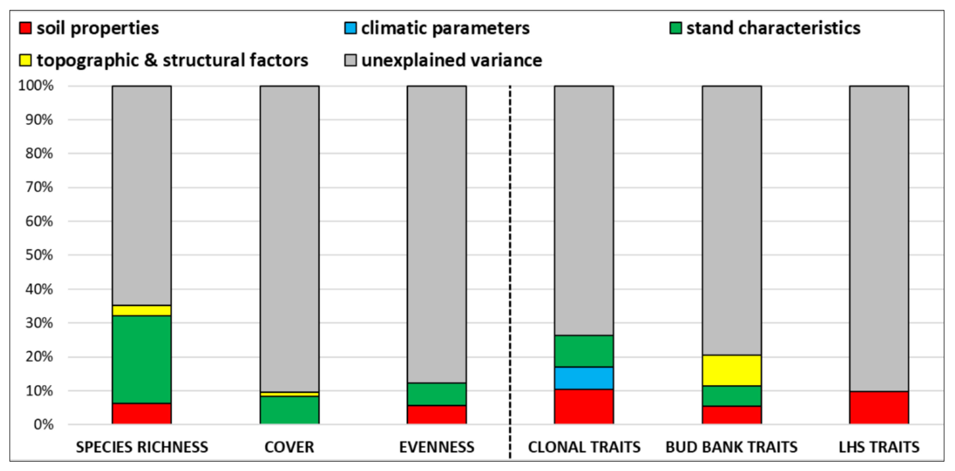
3.3. Variance Partitioning

The analysis of variance partitioning (Figure 8) revealed that the relative contribution (expressed in %) of soil properties towards explaining the variation in response variables was as follows: clonal traits (10.4%) > LHS traits (9.8%) > species richness (6.3%) > evenness (5.7%) > bud bank traits (5.5%) > herb-layer cover (0.0%). Climatic parameters explained 6.6% of the variation in clonal traits, while all other GAMs did not include any of the climatic parameters. In contrast, stand characteristics explained a substantial proportion of variation in species richness (25.0%) > clonal traits (9.4%) > herb-layer cover (8.3%) > evenness (6.6%) > bud bank traits (6.0%), but did not contribute to explaining the variation in LHS traits (0.0%). Topographic and structural factors proved to have an important role in explaining the variation in bud bank traits (9.0%), species richness (3.2%) and herb-layer cover (1.2%). However, these ecological drivers were not included in the GAMs for evenness, clonal traits and LHS traits (Figure 8).

Averaging these results together, forest stand characteristics on average explained the highest fraction (9.3%) of variation in all six response variables considered. The second most explanatory group of predictors was soil properties (6.3%), followed by topographic and structural factors (2.2%) and climatic parameters (1.1%). Looking at the three taxonomy-based diversity measures separately, the order of predictor groups from most to least important was as follows: stand characteristics (13.5%) > soil properties (4.0%) > topographic and structural factors (1.5%). Climatic parameters did not contribute to explaining the taxonomy-based measures. In the case of the three response variables describing functional trait diversity, the order changed in favor of soil properties (8.6%). The variation in trait groups was also strongly affected by stand characteristics (5.1%) and topographic and structural factors (3.0%) but less so by climatic parameters (2.2%).

4. Discussion

4.1. Species–Environment Relationships

Given that our study addresses the majority of forest types found in Central and SE Europe, the results are meaningful for similar European forests and also temperate forests in, e.g., Asia [100,101], North America [102,103,104] and other parts of the world [105]. We distinguished between three taxonomic response variables of herb-layer vegetation: species richness, herb-layer cover and species evenness. The first two have frequently been explored in many different forest types in the temperate zone around the globe [22,101,106], whereas species evenness has been examined to a much lesser degree.

Our findings indicate that shrub layer characteristics are important determinants for all three taxonomic response variables. Shrub layer species richness proved to be the most effective predictor of herb-layer richness and cover. This forest stand characteristic showed a positive effect on both variables. However, the increase in herb-layer richness along the gradient of shrub layer richness hit a plateau at high shrub-layer richness, suggesting competitive interactions between these two forest strata. Shrub-layer cover also proved significant for herb-layer species evenness. This again indicates the regulative role of the shrub layer, i.e., higher shrub cover prevents the domination of one or a few herb-layer species. In temperate forests, however, the shrub layer is often overlooked as it is assumed that shrubs are rather sparsely distributed under a dense tree canopy layer. This might be true in most cases, but the shrub layer likely acts as a direct filter for the herb-layer species underneath, particularly influencing light availability and the forest microclimate [107]. Although the shrub layer reduces forest floor light availability and contributes to higher litter production, its presence or absence may create highly variable microenvironments [108,109].

In contrast to the relative importance of the shrub layer in our monitoring plots, previous studies suggested that forest herb-layer vegetation is largely controlled by tree-layer characteristics. The authors of [106] found that tree species richness acts as a positive factor for herb-layer species richness and cover in mixed temperate forests in Hungary. None of our final GAMs included tree species richness as an explanatory variable. Instead, the proportion of broadleaves in the tree layer (a proxy for tree species composition) was a significant predictor in all three GAMs for taxonomy-based measures of diversity. The results indicated that a higher proportion of broadleaves tends to decrease herb-layer species richness and cover. At first glance, such patterns run counter to prevailing evidence in forest ecology.

In temperate and boreal zones, coniferous forests generally provide less diversified vascular understories than broadleaved forests [7]. This incongruence can be somewhat explained by the fact that our monitoring plots included some sites with pure conifer stands (e.g., Picea abies) growing on mixed parent material, which contributed to the coexistence of acidophilous species (present due to the thick litter layer from spruce trees that lowered the pH of the topsoil) and basophilous plants (occurring on less acidic microsites). On the other extreme, some stands were composed only of broadleaved tree species but had relatively low herb-layer richness. One typical example is the phytosociological association of Blechno-Fagetum, a species-poor beech community due to soils with low pH values and impoverished nutrients in the upper horizons. The observed importance of broadleaves (deciduous trees) might be related to seasonal variations of overstory canopy cover and associated herb-layer development. The compositional differences between spring and summer are relevant. It is important to note, however, that the summer aspect of herb-layer vegetation (capturing most of the seasonal variability of ground flora in temperate forests) was considered here. This sampling included both spring and summer species and is representative for these types of temperate forest.

Tree species composition was the most expressed predictor for herb-layer species evenness. The relationship between these two variables was evidently unimodal, suggesting that mixed forest stands support the highest herb-layer evenness. Mixed overstory canopy comprised of both broadleaves and conifers exhibits higher spatial and temporal variation of resources in the understory layer [21]. In contrast, the majority of the monodominant overstories in our dataset were characterized by the dominance of a single or a few herb-layer species.

Another important ecological determinant for herb-layer diversity was tree layer shade-casting ability, a proxy for light conditions at the forest floor. However, the results of our study suggest that species richness increased along the tree-layer shade-casting ability gradient, at least to a certain point—at the highest tree-layer SCA values, the non-linear curve started to bend down. This observation is slightly counterintuitive to the general expectation that more light at the forest floor would result in higher plant richness [110,111]. Light is the most important limiting factor in the majority of forest ecosystems [112], and shade tolerance affects the ability of plants to cope with other environmental stressors [20]. However, the effect of light is not straightforward because the diversity of the herb layer may not necessarily be in correlation with light availability. The authors of [13] noted that photosynthetically active radiation was of secondary importance for the distribution of widespread temperate forest herbs in beech forests on calcareous soils. In the study of [113], light conditions were the most important drivers in acidophilic beech-oak forests, while on more neutral forest sites different soil properties proved more determinant. Other studies (e.g., [25]) have also concluded that the effects of light availability depend on edaphic conditions.

One possible explanation is that on certain sites (pine forests in our case), higher light availability supports the expansion of plant species adapted to a high-light environment (e.g., grasses). Their dominance can lead to the competitive exclusion of less adapted and competitively inferior species, resulting in the impoverishment of community-level richness. Another reason for this pattern may, at least in part, lie in so-called “compensatory effects”. Compensation can be understood in the sense that more favorable soil conditions (higher soil pH and moisture) outweighed the effects of seemingly stressful abiotic conditions in the form of less available light (higher tree-layer SCA), resulting in high herb-layer species richness. Some of our study sites experienced more favorable light conditions due to the sparser canopy of certain tree species (e.g., Pinus sylvestris) but were at the same time characterized by acidic, nutrient-poor soils. At the other end of the light gradient, our plots included some forest stands dominated by broadleaves or mixed stands with closed tree-layer cover and late-successional tree species able to produce high shade (e.g., Fagus sylvatica, Abies alba). Many of such sites are, however, located on carbonate parent material with base rich calcareous soils, where higher soil pH facilitates plant species richness [114,115]. Shade-tolerant herbaceous perennials that give priority to persistence are the main growth form in the herb layer of these forest ecosystems. In addition, we did not consider plot-level environmental heterogeneity, which might contribute to species coexistence. Spatial variability in resources can be even more important for plant species richness than average site conditions [116,117]. Resource heterogeneity exerts a greater influence on vegetation diversity at the later stages of succession, i.e., in closed canopy mature forest stands [21]. Soil heterogeneity seems to be especially important for typical forest plant species [118]. Moreover, sun flecks can have a prominent effect on fine-scale patterning of herb-layer composition and diversity [119].

Our general observation regarding soil properties was that the organic soil layer was more important for herb-layer vegetation than mineral soil layers. Herb-layer species richness was positively related to increasing soil pH of the organic layer (similar to the work of [22] and [110]), a pattern which confirms that forest sites on limestone and dolomite bedrock with more calcareous soils (characterized by higher pH and cation exchange capacity) host higher plant diversity [114]. The authors of [120] reported that understory plant richness decreased significantly with increasing soil acidity. Another relation to soil properties in our plots was observed for herb-layer species evenness, which was negatively correlated with total nitrogen content in organic soils. This could suggest that herb-layer communities on more productive sites tend to be characterized by the prevalence of competitive nutrient-demanding species with vigorous growth, resulting in uneven distribution of abundances among dominant and subordinate species.

Climatic parameters and topographic and structural factors were, compared to forest stand characteristics and soil properties, relatively unimportant for taxonomy-based diversity measures of herb-layer communities. We assume that the climatic signal was weakly expressed due to the usage of broad-scale and interpolated climatic data rather than in-situ measurements. In the case of herb-layer species richness, the cover of rocks on the surface was positively associated with richness. This can be also interpreted in relation to bedrock and soil conditions as forest sites on carbonate parent material usually show higher surface rockiness. Focusing on herb-layer cover, moss cover on the forest soil was a significant predictor with a hump-shaped trend. This indicates that mosses can be both facilitative (creating favorable microsites for seedling establishment) and inhibitive (competition for growing space and resources) for the cover of herb-layer vascular plants. The only climatic parameter that was included in the final GAM for herb-layer cover was temperature seasonality, but even in this case, the effect was marginally significant.

4.2. Trait–Environment Relationships

Trait-based approaches increase universality and allow comparisons between different regions of the globe. Thus, we assume that our results related with functional diversity measures are likely more comparable with other studies [121,122] than findings about taxonomy-based measures.

Analyzing convergence and divergence in plant traits along ecological gradients [47,49] complements patterns observed on the taxonomic (species) level. The understanding of trait variation along environmental gradients is one of the main research directions in plant functional ecology [19]. We included three groups of plant functional traits: clonal traits, bud bank traits and traits belonging to the leaf-height-seed (LHS) scheme [80]. While above-ground LHS traits have been frequently studied, below-ground traits remain largely unexplored, and limited evidence exists in the scientific literature regarding forest herb-layer vegetation [41].

The diversity of clonal traits (clonality, clonal index, type of clonal growth organ, persistence of clonal organ) was most significantly driven by stand characteristics (shrub-layer richness), climatic parameters (precipitation seasonality) and soil properties (soil pH of the organic layer). The authors of [41] found that climate had a pervasive effect on determining patterns of clonal trait composition (not diversity) in Italian forest understories. The authors of [49] concluded that clonal traits were significantly more diverse in habitats that represented high soil reaction. Our results agree with this observation as we showed a shift from clonal trait convergence to divergence along the organic soil pH gradient. An interesting pattern was observed for soil texture. On sites with a higher proportion of clay in the upper mineral soil layer, clonal traits tended to converge (i.e., low dissimilarity among species regarding the clonal traits). One possible explanation could be that below-ground clonal organs have limited space for growth in soils where clay particles are more abundant, and soils are more compacted.

The diversity of bud bank traits (bud bank size and bud bank depth) was mainly related to altitude, organic soil pH, tree-layer SCA and, similar to clonal traits, to precipitation seasonality. However, bud bank trait diversity changed differently along the precipitation gradient compared to clonal traits. Furthermore, it is worth noting that altitude (here assigned to the group of topographic and structural factors) is actually a variable very closely associated with mean climatic conditions. Across our dataset, altitude exhibited a strong negative correlation with mean annual temperature (r = −0.94) and a positive correlation with precipitation (r = 0.43). Elevation played a major role in shaping plant diversity in the study of [42], where high-elevation plots exhibited reduced functional diversity of below-ground storage organs that may promote cold-tolerance. Our findings similarly suggest that the diversity of bud bank traits declined with altitude, meaning that bud bank trait divergence occurred at low-altitude sites with higher temperatures. This corroborates with the results of [49], who reported that bud bank traits were more diverse in warmer habitats. In addition, our results are also in line with theirs in terms of the dependence of below-ground traits on light conditions. Convergence of bud bank traits occurred in plots with higher tree-layer SCA, meaning that in forest understories with limited light availability, species seem to use similar clonal strategies to cope with shade.

Compared to clonal and bud bank traits, LHS traits were significantly associated with only two soil properties: soil pH and nitrogen content of the organic layer. In their study of LHS trait composition (not diversity) across understory plant communities in Italian forests, the authors of [40] summarized that climate-related factors as well as soil nitrogen and phosphorus availability were the explanatory variables most correlated to trait variation. They explicitly highlighted the need to integrate soil properties as local drivers of above-ground trait diversity. In our case, the diversity of LHS traits decreased along the soil pH and productivity gradient. This agrees with the work of [49] who found a negative correlation between soil reaction and LHS trait diversity over a large set of temperate vegetation types. Furthermore, we have additionally observed an interesting pattern regarding this trait group across our monitoring plots. While clonal and bud bank trait diversity were positively associated with herb-layer species richness, for LHS traits the relationship was negative (results not shown). This suggests that species-poor herb-layer communities tend to be functionally more diverse than species-rich communities, pointing to the conclusion that species richness is not always a good surrogate for functional diversity. Moreover, stronger filtering of LHS traits occurred in environments (forest sites) with sufficient nutrient levels but are generally less favorable in terms of light availability, such as dense beech or mixed broadleaf forests on more fertile soil types.

5. Conclusions

This work investigated the effects of ecological drivers on the vascular plant diversity of herb-layer communities in Slovenian forests. The main strengths of our study are (1) the use of harmonized ICP Forests vegetation records accompanied with detailed in-situ measurements of soil properties and estimations of a wide variety of ecological factors as potential predictors and (2) the inclusion of taxonomy- and trait-based measures of diversity. Moreover, within each diversity facet, three different response variables were distinguished. To date, only a few studies (e.g., [42]) have simultaneously tested the impacts of environmental drivers on both taxonomic and functional aspects. Most studies have focused on comparing species (trait) richness and (functional) composition (e.g., [5,120]) rather than on integrating multiple facets of diversity. Disentangling the relative importance of ecological drivers for different organizational levels can elucidate how abiotic constraints influence plant community assembly and potentially have implications for forest biodiversity conservation and management of forests.

Variance partitioning analyses revealed the prevalent effect of forest stand characteristics and soil properties on the majority of investigated taxonomic and functional trait variables. Some common patterns emerged. One evident example was the lack of a climatic signal for taxonomy-based measures of diversity. Although we can draw such general conclusions based on the comparison between taxonomy- and trait-based diversity measures, it is important to note that even within the same diversity facet (taxonomic and functional), each response variable responded quite differently to ecological factors.

Our next research step will be dedicated to the quantification of how species (e.g., using ordination methods) and functional composition (e.g., by combining the fourth-corner and the RLQ method; [121,123]) of herb-layer communities are related to ecological drivers. We encourage researchers from other countries involved in the ICP Forests monitoring network to take a similar multi-faceted approach by systematically including functional diversity instead of taxonomic metrics only and maintain that this should be incorporated into biodiversity monitoring plans [42]. Comprehensive comparisons will not only reveal factors influencing species and functional trait diversity but can also provide useful insights related to relevant drivers of temporal dynamics in European forest plant communities, particularly in the face of global environmental change and the biodiversity crisis [4,24,117].

References

1. Van der Maarel, E. Vegetation Ecology; Blackwell Publishing: Oxford, UK, 2005; 408p. [Google Scholar]
2. Zhang, Y.; Chen, H.Y.H.; Taylor, A. Multiple drivers of plant diversity in forest ecosystems. Glob. Ecol. Biogeogr. 2014, 23, 885–893. [Google Scholar] [CrossRef]
3. Sabatini, F.M.; Jiménez-Alfaro, B.; Burrascano, S.; Blasi, C. Drivers of herb-layer species diversity in two unmanaged temperate forest in northern Spain. Community Ecol. 2014, 15, 147–157. [Google Scholar] [CrossRef]
4. Maes, S.L.; Perring, M.P.; Depauw, L.; Bernhardt-Römermann, M.; Blondeel, H.; Brūmelis, G.; Brunet, J.; Decocq, G.; den Ouden, J.; Govaert, S.; et al. Plant functional trait response to environmental drivers across European temperate forest understorey communities. Plant Biol. 2020, 22, 410–424. [Google Scholar] [CrossRef] [PubMed]
5. Vanneste, T.; Valdés, A.; Verheyen, K.; Perring, M.P.; Bernhardt-Römermann, M.; Andrieu, E.; Brunet, J.; Cousins, S.A.O.; Deconchat, M.; De Smedt, P.; et al. Functional trait variation of forest understory plant communities across Europe. Basic Appl. Ecol. 2019, 34, 1–14. [Google Scholar] [CrossRef]
6. Weigel, R.; Gilles, J.; Klisz, M.; Manthey, M.; Kreyling, J. Forest understory vegetation is more related to soil than to climate towards the cold distribution margin of European beech. J. Veg. Sci. 2019, 30, 746–755. [Google Scholar] [CrossRef]
7. Barbier, S.; Gosselin, F.; Balandier, P. Influence of tree species on understory vegetation diversity and mechanisms involved—A critical review for temperate and boreal forests. Forest Ecol. Manag. 2008, 254, 1–15. [Google Scholar] [CrossRef]
8. Petersson, L.; Holmström, E.; Lindbladh, M.; Felton, A. Tree species impact on understory vegetation: Vascular plant communities of Scots pine and Norway spruce managed stands in northern Europe. Forest Ecol. Manag. 2019, 448, 330–345. [Google Scholar] [CrossRef]
9. Axmanová, I.; Chytrý, M.; Zelený, D.; Li, C.-F.; Vymazalova, M.; Danihelka, J.; Horsák, M.; Kočí, M.; Kubešová, S.; Lososová, Z.; et al. The species richness-productivity relationship in the herb layer of European deciduous forests. Global Ecol. Biogeogr. 2012, 21, 657–667. [Google Scholar] [CrossRef]
10. Hulshof, C.M.; Spasojevic, M.J. The edaphic control of plant diversity. Global Ecol. Biogeogr. 2020, 29, 1634–1650. [Google Scholar] [CrossRef]
11. Catorci, A.; Tardella, F.M.; Cutini, M.; Luchetti, L.; Paura, B.; Vitanzi, A. Reproductive traits variation in the herb layer of a submediterranean deciduous forest landscape. Plant Ecol. 2013, 214, 737–749. [Google Scholar] [CrossRef]
12. Tardella, F.M.; Postiglione, N.; Bricca, A.; Cutini, M.; Catorci, A. Altitude and aspect filter the herb layer functional structure of sub-Mediterranean forests. Phytocoenologia 2019, 49, 185–198. [Google Scholar] [CrossRef]
13. Leuschner, C.; Lendzion, J. Air humidity, soil moisture and soil chemistry as determinants of the herb layer composition in European beech forests. J. Veg. Sci. 2009, 20, 288–298. [Google Scholar] [CrossRef]
14. Macek, M.; Kopecký, M.; Wild, J. Maximum air temperature controlled by landscape topography affects plant species composition in temperate forests. Landscape Ecol. 2019, 34, 2541–2556. [Google Scholar] [CrossRef]
15. Tinya, F.; Márialigeti, S.; Király, I.; Németh, B.; Ódor, P. The effect of light conditions on herbs, bryophytes and seedlings of temperate mixed forests in Őrség, Western Hungary. Plant Ecol. 2009, 204, 69–81. [Google Scholar] [CrossRef]
16. Landuyt, D.; Perring, M.P.; Seidl, R.; Tauber, F.; Verbeeck, H.; Verheyen, K. Modelling understorey dynamics in temperate forests under global change–Challenges and perspectives. Perspect. Plant Ecol. Syst. 2018, 31, 44–54. [Google Scholar] [CrossRef] [PubMed] [Green Version]
17. Whigham, D.E. Ecology of woodland herbs in temperate deciduous forests. Annu. Rev. Ecol. Evol. Syst. 2004, 35, 583–621. [Google Scholar] [CrossRef] [Green Version]
18. Tinya, F.; Márialigeti, S.; Bidló, B.; Ódor, P. Environmental drivers of the forest regeneration in temperate mixed forests. Forest Ecol. Manag. 2019, 433, 720–728. [Google Scholar] [CrossRef] [Green Version]
19. Leuschner, C.; Meier, I.C. The ecology of Central European tree species: Trait spectra, functional trade-offs, and ecological classification of adult trees. Perspect. Plant Ecol. 2018, 33, 89–103. [Google Scholar] [CrossRef]
20. Valladares, F.; Laanisto, L.; Niinemets, Ü.; Zavala, M.A. Shedding light on shade: Ecological perspectives of understorey plant life. Plant Ecol. Divers. 2016, 9, 237–251. [Google Scholar] [CrossRef] [Green Version]
21. Su, X.; Wang, M.; Huang, Z.; Fu, S.; Chen, H.Y.H. Forest Understory Vegetation: Colonization and the Availability and Heterogeneity of Resources. Forests 2019, 10, 944. [Google Scholar] [CrossRef] [Green Version]
22. Vockenhuber, E.A.; Scherber, C.; Lagenbruch, C.; Meißner, M.; Seidel, D.; Tscharntke, T. Tree diversity and environmental context predict herb species richness and cover in Germany’s largest connected deciduous forest. Perspect. Plant Ecol. 2011, 13, 111–119. [Google Scholar] [CrossRef]
23. Depauw, L.; Perring, M.P.; Landuyt, D.; Maes, S.L.; Blondeel, H.; De Lombaerde, E.; Brūmelis, G.; Brunet, J.; Closset-Kopp, D.; Decocq, G.; et al. Evaluating structural and compositional canopy characteristics to predict the light-demand signature of the forest understorey in mixed, semi-natural temperate forests. Appl. Veg. Sci. 2021, 24, e12532. [Google Scholar] [CrossRef]
24. Depauw, L.; Perring, M.P.; Landuyt, D.; Maes, S.L.; Blondeel, H.; De Lombaerde, E.; Brūmelis, G.; Brunet, J.; Closset-Kopp, D.; Czerepko, J.; et al. Light availability and land-use history drive biodiversity and functional changes in forest herb layer communities. J. Ecol. 2020, 108, 1411–1425. [Google Scholar] [CrossRef]
25. Mölder, A.; Streit, M.; Schmidt, W. When beech strikes back: How strict nature conservation reduces herb-layer diversity and productivity in Central European deciduous forests. Forest Ecol. Manag. 2014, 319, 51–61. [Google Scholar] [CrossRef]
26. De Vries, W.; Reinds, G.J.; Deelstra, H.D.; Klap, J.M.; Vel, E.M. Intensive Monitoring of Forest Condition in Europe: Technical Report 2000; UN/ECE EC: Brussels, Belgium; Geneva, Switzerland, 2000; p. 193. Available online: https://www.icp-forests.org/pdf/TRLII2000.pdf (accessed on 1 December 2020).
27. De Vries, W.; Vel, E.M.; Reinds, G.J.; Deelstra, H.; Klap, J.M.; Leeters, E.E.J.M.; Hendriks, C.M.A.; Kerkvoorden, M.; Landmann, G.; Herkendell, J.; et al. Intensive monitoring of forest ecosystems in Europe. 1. Objectives, set-up and evaluation strategy. For. Ecol. Manag. 2003, 174, 77–95. [Google Scholar] [CrossRef]
28. Rautio, P.; Ferretti, M. Monitoring European forests: Results from science, policy, and society. Ann. For. Sci. 2015, 72, 875–876. [Google Scholar] [CrossRef] [Green Version]
29. Gilliam, F.S. The ecological significance of the herbaceous layer in temperate forest ecosystems. Bioscience 2007, 57, 845–858. [Google Scholar] [CrossRef]
30. Thrippleton, T.; Bugmann, H.; Kramer-Priewasser, K.; Snell, R.S. Herbaceous understorey: An overlooked player in forest landscape dynamics? Ecosystems 2016, 19, 1–15. [Google Scholar] [CrossRef]
31. Spicer, M.E.; Mellor, H.; Carson, W.P. Seeing beyond the trees: A comparison of tropical and temperate growth forms and their vertical distribution. Ecology 2020, 101, e02974. [Google Scholar] [CrossRef]
32. Landuyt, D.; De Lombaerde, E.; Perring, M.P.; Hertzog, L.R.; Ampoorter, E.; Maes, S.L.; De Frenne, P.; Ma, S.; Proesmans, W.; Blondeel, H.; et al. The functional role of temperate forest understorey vegetation in a changing world. Glob. Change Biol. 2019, 25, 3625–3641. [Google Scholar] [CrossRef] [PubMed]
33. Canullo, R.; Starlinger, F.; Granke, O.; Fischer, R.; Aamlid, D.; Neville, P. ICP Forests Manual on Methods and Criteria for Harmonized Sampling, Assessment, Monitoring and Analysis of the Effects of Air Pollution on Forests; Part VII.1: Assessment of Ground Vegetation; UNECE ICP Forests Programme Coordinating Centre: Hamburg, Germany, 2011; p. 19. Available online: https://www.icp-forests.org/pdf/manual/2016/ICP_Manual_2016_01_part07-1.pdf (accessed on 1 December 2020).
34. Thimonier, A.; Kull, P.; Keller, W.; Moser, B.; Wohlgemuth, T. Ground vegetation monitoring in Swiss forests: Comparison of survey methods and implications for trend assessments. Environ. Monit. Assess. 2011, 174, 47–63. [Google Scholar] [CrossRef] [PubMed]
35. Seidling, W.; Hamber, L.; Máliš, F.; Salemaa, M.; Kutnar, L.; Czerepko, J.; Kompa, T.; Buriánek, V.; Dupouey, J.-L.; Vodálova, A.; et al. Comparing observer performances in vegetation records by efficiency graphs derived from rarefaction curves. Ecol. Indic. 2020, 109, 105790. [Google Scholar] [CrossRef]
36. Dirnböck, T.; Grandin, U.; Bernhardt-Römermann, M.; Beudert, B.; Canullo, R.; Forsius, M.; Grabner, M.-T.; Holmberg, M.; Kleemola, S.; Lundin, L.; et al. Forest floor vegetation response to nitrogen deposition in Europe. Glob. Change Biol. 2014, 20, 429–440. [Google Scholar] [CrossRef]
37. van Dobben, H.; de Vries, W. The contribution of nitrogen deposition on the eutrophication signal in understory plant communities of European forests. Ecol. Evol. 2017, 7, 214–227. [Google Scholar] [CrossRef] [PubMed] [Green Version]
38. Novotný, R.; Buriánek, V.; Šrámek, V.; Hůnová, I.; Skořepova, I.; Zapletal, M.; Lomský, B. Nitrogen deposition and its impact on forest ecosystems in the Czech Republic–change in soil chemistry and ground vegetation. iForest 2016, 10, 48–54. [Google Scholar] [CrossRef] [Green Version]
39. Kutnar, L.; Nagel, T.A.; Kermavnar, J. Effects of Disturbance on Understory Vegetation across Slovenian Forest Ecosystems. Forests 2019, 10, 1048. [Google Scholar] [CrossRef] [Green Version]
40. Chelli, S.; Simonetti, E.; Wellstein, C.; Campetella, G.; Carnicelli, S.; Andreetta, A.; Giorgini, D.; Puletti, N.; Bartha, S.; Canullo, R. Effects of climate, soil, forest structure and land use on the functional composition of the understorey in Italian forests. J. Veg. Sci. 2019, 30, 1110–1121. [Google Scholar] [CrossRef]
41. Chelli, S.; Ottaviani, G.; Simonetti, E.; Wellstein, C.; Canullo, R.; Carnicelli, S.; Andreetta, A.; Puletti, N.; Bartha, S.; Cervellini, M.; et al. Climate is the main driver of clonal and bud bank traits in Italian forest understories. Perspect. Plant Ecol. 2019, 40, 125478. [Google Scholar] [CrossRef] [Green Version]
42. Ottaviani, G.; Götzenberger, L.; Bacaro, G.; Chiarucci, A.; de Bello, F.; Marcantonio, M. A multifaceted approach for beech forest conservation: Environmental drivers of understory plant diversity. Flora 2019, 256, 85–91. [Google Scholar] [CrossRef]
43. Bricca, A.; Chelli, S.; Canullo, R.; Cutini, M. The legacy of the past logging: How forest structure affects different facets of understory plant diversity in abandoned coppice forests. Diversity 2020, 12, 109. [Google Scholar] [CrossRef] [Green Version]
44. Padullés Cubino, J.; Lososová, Z.; Bonari, G.; Agrillo, E.; Attore, F.; Bergmeier, E.; Biurrun, I.; Campos, J.A.; Čarni, A.; Ćuk, M.; et al. Phylogenetic structure of European forest vegetation. J. Biogeogr. 2021. Early view. [Google Scholar] [CrossRef]
45. Padullés Cubino, J.; Jiménez-Alfaro, B.; Sabatini, F.M.; Willner, W.; Lososová, Z.; Biurrun, I.; Brunet, J.; Campos, J.A.; Indreica, A.; Jansen, F.; et al. Plant taxonomic and phylogenetic turnover increases toward climatic extremes and depends on historical factors in European beech forests. J. Veg. Sci. 2021, 32, e12977. [Google Scholar] [CrossRef]
46. Cadotte, M.W.; Carscadden, K.; Mirotchnick, N. Beyond species: Functional diversity and the maintenance of ecological processes and services. J. Appl. Ecol. 2011, 48, 1079–1087. [Google Scholar] [CrossRef]
47. Fraser, L.H.; Garris, H.W.; Carlyle, C.N. Predicting plant trait similarity along environmental gradients. Plant Ecol. 2016, 217, 1297–1306. [Google Scholar] [CrossRef]
48. Naaf, T.; Wulf, M. Plant community assembly in temperate forests along gradients in soil fertility and disturbance. Acta Oecol. 2012, 39, 101–108. [Google Scholar] [CrossRef]
49. Vojtkó, A.E.; Freitag, M.; Bricca, A.; Martello, F.; Compañ, J.M.; Küttim, M.; Kun, R.; de Bello, F.; Klimešová, J.; Götzenberger, L. Clonal vs leaf-height-seed (LHS) traits: Which are filtered more strongly across habitats? Folia Geobot. 2017, 52, 269–281. [Google Scholar] [CrossRef]
50. Klimešová, J.; Herben, T. Clonal and bud bank traits: Patterns across temperate plant communities. J. Veg. Sci. 2015, 26, 243–253. [Google Scholar] [CrossRef]
51. Klimešová, J.; Tackenberg, O.; Herben, T. Herbs are different: Clonal and bud bank traits can matter more than leaf-height-seed traits. New Phytol. 2016, 210, 13–17. [Google Scholar] [CrossRef] [PubMed] [Green Version]
52. Kutnar, L. Diversity of woody species on forest monitoring plots in Slovenia. GozdVestn 2011, 69, 271–278, (In Slovenian with English Summary). [Google Scholar]
53. Urbančič, M.; Kutnar, L.; Kobal, M.; Žlindra, D.; Marinšek, A.; Simončič, P. Soil and vegetation characteristics on Intensive Monitoring Plots of forest ecosystems). GozdVestn 2016, 74, 3–27, (In Slovenian with English Summary). [Google Scholar]
54. Kermavnar, J.; Kutnar, L. Patterns of understory community assembly and plant trait-environment relationships in temperate SE European Forests. Diversity 2020, 12, 91. [Google Scholar] [CrossRef] [Green Version]
55. WorldClim. Global Climate and Weather Data. 2021. Available online: https://www.worldclim.org/ (accessed on 15 November 2020).
56. Slovenia Forest Service. Annual Report of Slovenia Forest Service for Year 2019; Slovenia Forest Service: Ljubljana, Slovenia, 2019. (In Slovenian) [Google Scholar]
57. Forest Europe. State of Europe’s Forests 2020. Available online: https://foresteurope.org/publications/ (accessed on 1 December 2020).
58. Kutnar, L.; Veselič, Ž.; Dakskobler, I.; Robič, D. Typology of Slovenian forest sites according to ecological and vegetation conditions for the purpose of forest management. GozdVestn 2012, 70, 195–214, (In Slovenian with English Summary). [Google Scholar]
59. Bončina, A.; Rozman, A.; Dakskobler, I.; Klopčič, M.; Babij, V.; Poljanec, A. Gozdni rastiščni tipi Slovenije–Vegetacijske, sestojne in upravljavske značilnosti; University of Ljubljana, Biotechnical Faculty, Department of Forestry and Renewable forest resources, Slovenia Forest Service: Ljubljana, Slovenia, 2021. [Google Scholar]
60. Barkman, J.J.; Doing, H.S.; Segal, S. Kritische Bemerkungen und Vorschläge zur quantitativen Vegetationsanalyse. Acta Bot. Neerl. 1964, 13, 394–419. [Google Scholar] [CrossRef]
61. Tutin, T.G.; Heywood, V.H.; Burges, N.A.; Moore, D.M.; Valentine, D.H.; Walters, S.M.; Webb, D.A. Flora Europaea; Cambridge University Press: Cambridge, UK, 1964–1980; Volume 1–5.
62. Tutin, T.G.; Burges, N.A.; Chater, A.O.; Edmondson, J.R.; Heywood, V.H.; Moore, D.M.; Valentine, D.H.; Walters, S.M.; Webb, D.A. Flora Europaea, 2nd ed.; Cambridge University Press: Cambridge, UK, 1993. [Google Scholar]
63. Martinčič, A.; Wraber, T.; Jogan, N.; Podobnik, A.; Turk, B.; Vreš, B.; Ravnik, V.; Frajman, B.; Strgulc Krajšek, S.; Trčak, B.; et al. Mala Flora Slovenije: Ključ za določanje praprotnic in semenk; Tehniška založba Slovenije: Ljubljana, Slovenia, 2007; p. 967. [Google Scholar]
64. WGFB. The BioSoil Forest Biodiversity Field Manual, version 1.0/1.1/1.1a for the field assessment 2006-07; Evaluation of BioSoil Demonstration Project: Forest Biodiversity; JRC–Inst. for Environment and Sustainability, Ed.; Publications Office of the European Union: Luxembourg, 2011; pp. 81–102. [Google Scholar] [CrossRef]
65. Urbančič, M.; Kutnar, L.; Kralj, T.; Kobal, M.; Simončič, P. Site characteristics of permanent plots on the Slovenian 16 km × 16 km net. GozdVestn 2009, 67, 17–48, (In Slovenian with English Summary). Available online: https://www.dlib.si/stream/URN:NBN:SI:DOC-OFRDZTK5/76e434ce-10e9-48d5-809b-6b7d367a291f/PDF (accessed on 1 October 2020).
66. Bastrup-Birk, A.; Neville, P.; Chirici, G.; Houston, T. The BioSoil—Forest Biodiversity; Field Manual, Ver. 1.0/1.1/1.1a; for the field assessment 2006–07, Forest Focus Demonstration Project; BioSoil, Forest Research: Farnham, UK, 2007; 51p. [Google Scholar]
67. ICP Forests. Manual on Methods and Criteria for Harmonized Sampling, Assessment, Monitoring and Analysis of the Effects of Air Pollution on Forests. Part IIIa. Sampling and Analysis of Soil. UN ECE Convention on Long-Range Transboundary Air Pollution. International Co-operative Programme on Assessment and Monitoring of Air Pollution Effects on Forests. Expert Panel on Soil; Forest Soil Co-ordinating Centre, Research Institute for Nature and Forest: Geraardsbergen, Belgium, 2006; 127p. [Google Scholar]
68. Maes, S.L.; Blondeel, H.; Perring, M.P.; Depauw, L.; Brūmelis, G.; Brunet, J.; Decocq, G.; den Ouden, J.; Härdtle, W.; Hédl, R.; et al. Litter quality, land-use history, and nitrogen deposition effects on topsoil conditions across European temperate deciduous forests. Forest Ecol. Manag. 2019, 433, 405–418. [Google Scholar] [CrossRef] [Green Version]
69. Fick, S.E.; Hijmans, R.J. WorldClim 2: New 1-km spatial resolution climate surfaces for global land areas. Int. J. Climat. 2017, 37, 4302–4315. [Google Scholar] [CrossRef]
70. Trabucco, A.; Zomer, R.J. Global Aridity Index (Global-Aridity) and Global Potential Evapo-Transpiration (Global-PET) Geospatial Database. CGIAR Consortium for Spatial Information. 2009. Published online. Available online: http://www.csi.cgiar.org (accessed on 15 November 2020).
71. Hijmans, R.J.; van Etten, J.; Sumner, M.; Cheng, J.; Baston, D.; Bevan, D.; Bivand, R.; Bussetto, L.; Canty, M.; Fasoil, B.; et al. Package “Raster”–Geographic Data Analysis and Modelling; Version 3.4-5; 2020. Available online: https://cran.r-project.org/web/packages/raster/index.html (accessed on 15 November 2020).
72. Closset-Kopp, D.; Hattab, T.; Decocq, G. Do drivers of forestry vehicles also drive herb layer changes (1970–2015) in a temperate forest with contrasting habitat and management conditions? J. Ecol. 2019, 107, 1439–1456. [Google Scholar] [CrossRef] [Green Version]
73. Ricotta, C.; Moretti, M. CWM and Rao’s quadratic diversity: A unified framework for functional ecology. Oecologia 2011, 167, 181–188. [Google Scholar] [CrossRef] [PubMed]
74. Geiger, R. The Climate Near the Ground; Harvard University Press: Cambridge, MA, USA, 1966. [Google Scholar]
75. Pielou, E.C. Ecological Diversity; Wiley & Sons: New York, NY, USA, 1975. [Google Scholar]
76. Oksanen, J.; Blanchet, F.G.; Friendly, M.; Kindt, R.; Legendre, P.; McGlinn, D.; Minchin, P.R.; O’Hara, R.B.; Simpson, G.L.; Solymos, P.; et al. Package ‘vegan’—Community Ecology Package. 2019. Available online: https://cran.r-project.org/web/packages/vegan/vegan.pdf (accessed on 15 November 2020).
77. Stirling, G.; Wilsey, B. Empirical Relationships between Species Richness, Evenness, and Proportional Diversity. Am. Nat. 2001, 158, 286–299. [Google Scholar] [CrossRef] [PubMed]
78. Campetella, G.; Chelli, S.; Simonetti, E.; Damiani, C.; Bartha, S.; Wellstein, C.; Giorgini, D.; Puletti, N.; Mucina, L.; Cervellini, M.; et al. Plant functional traits are correlated with species persistence in the herb layer of old-growth beech forests. Sci. Rep. 2020, 10, 19253. [Google Scholar] [CrossRef]
79. Herben, T.; Klimešová, J.; Chytrý, M. Effects of disturbance frequency and severity on plant traits: An assessment across a temperate flora. Funct. Ecol. 2018, 32, 799–808. [Google Scholar] [CrossRef]
80. Westoby, M. A leaf-height-seed (LHS) plant ecology strategy scheme. Plant Soil 1998, 199, 213–227. [Google Scholar] [CrossRef]
81. Westoby, M.; Falster, D.S.; Moles, A.T.; Vesk, P.A.; Wright, I.J. Plant ecological strategies: Some leading dimensions of variation between species. Annual Rev. Ecol. Syst. 2002, 33, 125–159. [Google Scholar] [CrossRef] [Green Version]
82. Chelli, S.; Ottaviani, G.; Simonetti, E.; Campetella, G.; Wellstein, C.; Bartha, S.; Cervellini, M.; Canullo, R. Intraspecific variability of specific leaf area fosters the persistence of understorey specialists across a light availability gradient. Plant Biol. 2021, 23, 212–216. [Google Scholar] [CrossRef] [PubMed]
83. Klimešová, J.; de Bello, F. CLO-PLA: The database of clonal and bud bank traits of Central European flora. J. Veg. Sci. 2009, 20, 511–516. [Google Scholar] [CrossRef]
84. Klimešová, J.; Danihelka, J.; Chrtek, J.; de Bello, F.; Herben, T. CLO-PLA: A database of clonal and bud bank traits of Central European flora. Ecology 2017, 98, 1179. [Google Scholar] [CrossRef] [Green Version]
85. Chytrý, M.; Danihelka, J.; Kaplan, Z.; Wild, J.; Holubová, D.; Novotný, P.; Řezníčková, M.; Rohn, M.; Dřevojan, P.; Grulich, V. Pladias Database of the Czech Flora and Vegetation. Preslia 2021, 93, 1–87. [Google Scholar] [CrossRef]
86. Kleyer, M.; Bekker, R.M.; Knevel, I.C.; Bakker, J.P.; Thompson, K.; Sonnenschein, M.; Poschlod, P.; van Groenendael, J.M.; Klimeš, L.; Klimešová, J.; et al. The LEDA traitbase: A database of life-history traits of the Northwest European flora. J. Ecol. 2008, 96, 1266–1274. [Google Scholar] [CrossRef]
87. Botta-Dukát, Z. Rao’s quadratic entropy as a measure of functional diversity based on multiple traits. J. Veg. Sci. 2005, 16, 533–540. [Google Scholar] [CrossRef]
88. Schleuter, D.; Daufresne, M.; Massol, F.; Argiller, C. A user’s guide to functional diversity indices. Ecol. Monogr. 2010, 80, 469–484. [Google Scholar] [CrossRef] [Green Version]
89. Gower, J.C. A general coefficient of similarity and some of its properties. Biometrics 1971, 27, 857–871. Available online: https://www.jstor.org/stable/2528823 (accessed on 15 January 2021). [CrossRef]
90. De Bello, F.; Botta-Dukát, Z.; Lepš, J.; Fibich, P. Towards a more balanced combination of multiple traits when computing functional differences between species. Methods Ecol. Evol. 2020, 12, 443–448. [Google Scholar] [CrossRef]
91. Laliberté, E.; Legendre, P.; Shipley, B. Package “FD”: Measuring Functional Diversity (FD) from Multiple Traits, and Other Tools for Functional Ecology, R Package Version 1.0–12. 2015. Available online: https://cran.r-project.org/web/packages/FD/FD.pdf (accessed on 1 November 2020).
92. R Core Team. R: A Language and Environment for Statistical Computing; R Foundation for Statistical Computing: Vienna, Austria, 2019; Available online: https://www.R-project.org/ (accessed on 1 November 2020).
93. Hastie, T.; Tibshirani, R. Generalized Additive Models; Chapman and Hall (CRC Press): London, UK, 1991. [Google Scholar]
94. Yee, T.W.; Mitchell, N.D. Generalized additive models in plant ecology. J. Veg. Sci. 1991, 2, 587–602. [Google Scholar] [CrossRef]
95. Wood, S. Package ‘mgcv’–Mixed GAM computation Vehicle with Automatic Smoothness Estimation. 2020. Available online: https://cran.r-project.org/web/packages/mgcv/index.html (accessed on 1 December 2020).
96. Marra, G.; Wood, S. Practical variable selection for generalized additive models. Comput. Stat. Data An. 2011, 55, 2372–2387. [Google Scholar] [CrossRef]
97. Peterson, R.A. Package ‘bestNormalize’–Normalizing Transformation Functions, version 1.6.1. 2020. Available online: https://cran.r-project.org/web/packages/bestNormalize/index.html (accessed on 1 December 2020).
98. Borcard, D.; Legendre, P.; Drapeau, P. Partialling out the spatial component of ecological variation. Ecology 1992, 73, 1045–1055. [Google Scholar] [CrossRef] [Green Version]
99. Pakeman, R.J.; Lepš, J.; Kleyer, M.; Lavorel, S.; Garnier, E.; the VISTA consortium. Relative climatic, edaphic and management controls of plant functional trait signatures. J. Veg. Sci. 2009, 20, 148–159. [Google Scholar] [CrossRef]
100. Lee, C.-B.; Chun, J.-H. Environmental drivers of Patterns of Plant Diversity along a Wide Environmental Gradient in Korean Temperate Forests. Forests 2016, 7, 19. [Google Scholar] [CrossRef] [Green Version]
101. Černý, T.; Doležal, J.; Janeček, Š.; Šrůtek, M.; Valachovič, M.; Petřík, P.; Altman, J.; Bartoš, M.; Song, J.-S. Environmental correlates of plant diversity in Korean temperate forests. Acta Oecol. 2013, 47, 37–45. [Google Scholar] [CrossRef]
102. Gilliam, F.S. Excess Nitrogen in Temperate Forest Ecosystems Decrease Herbaceous Layer Diversity and Shifts Control from Soil to Canopy Structure. Forests 2019, 10, 66. [Google Scholar] [CrossRef] [Green Version]
103. Small, C.J.; McCarthy, B.C. Relationship of understory diversity to soil nitrogen, topographic variation, and stand age in an eastern oak forest, USA. Forest Ecol. Manag. 2005, 217, 229–243. [Google Scholar] [CrossRef]
104. Burton, J.I.; Mladenoff, D.J.; Clayton, M.K.; Forrester, J.A. The roles of environmental filtering and colonization in the fine-scale spatial patterning of ground-layer plant communities in north temperate deciduous forests. J. Ecol. 2011, 99, 764–776. [Google Scholar] [CrossRef]
105. Simpson, A.H.; Richardson, S.J.; Laughlin, D.C. Soil-climate interactions explain variation in foliar, stem, root and reproductive traits across temperate forests. Global Eol. Biogeogr. 2016, 25, 964–978. [Google Scholar] [CrossRef]
106. Márialigeti, S.; Tinya, F.; Bidló, A.; Ódor, P. Environmental drivers of the composition and diversity of the herb layer in mixed temperate forests in Hungary. Plant Ecol. 2016, 217, 549–563. [Google Scholar] [CrossRef] [Green Version]
107. Kovács, B.; Tinya, F.; Ódor, P. Stand structural drivers of microclimate in mature temperate mixed forests. Agr. Forest Meteorol. 2017, 234–235, 11–21. [Google Scholar] [CrossRef] [Green Version]
108. Bartels, S.F.; Chen, H.Y.H. Interactions between overstorey and understorey vegetation along an overstorey compositional gradient. J. Veg. Sci. 2013, 24, 543–552. [Google Scholar] [CrossRef]
109. Koorem, K.; Moora, M. Positive association between understory species richness and a dominant shrub species (Corylus avellana) in a boreonemoral spruce forest. For. Ecol. Manag. 2010, 260, 1407–1413. [Google Scholar] [CrossRef]
110. Hofmeister, J.; Hošek, J.; Modrý, J.; Roleček, J. The influence of light and nutrient availability on herb layer species richness in oak-dominated forests in central Bohemia. Plant Ecol. 2009, 205, 57–75. [Google Scholar] [CrossRef]
111. Dormann, C.F.; Bagnara, M.; Boch, S.; Hinderling, J.; Janeiro-Otero, A.; Schäfer, D.; Schall, P.; Hartig, F. Plant species richness increases with light availability, but not variability, in temperate forests understorey. BMC Ecol. 2020, 20, 43. [Google Scholar] [CrossRef]
112. Neufeld, H.S.; Young, D.R. Ecophysiology of the Herbaceous Layer in Temperate Deciduous Forests. In The Herbaceous Layer in Forests of Eastern North America; Gilliam, F.S., Ed.; Oxford University Press: New York, NY, USA, 2014; pp. 35–95. [Google Scholar]
113. Härdtle, W.; von Oheimb, G.; Westphal, C. The effects of light and soil conditions on the species richness of the ground vegetation of deciduous forests in northern Germany (Schleswig-Holstein). Forest Ecol. Manag. 2003, 182, 327–338. [Google Scholar] [CrossRef]
114. Ewald, J. The calcareous riddle: Why are there so many calciphilous species in the Central European flora? Folia Geobot. 2003, 38, 357–366. [Google Scholar] [CrossRef]
115. Schuster, B.; Diekmann, M. Changes in species density along the soil pH gradient–Evidence from German plant communities. Folia Geobot. 2003, 38, 367–379. [Google Scholar] [CrossRef]
116. Costanza, J.K.; Moody, A.; Peet, R.K. Multi-scale environmental heterogeneity as a predictor of plant species richness. Landscape Ecol. 2011, 26, 851–864. [Google Scholar] [CrossRef]
117. Gilliam, F.S. Response of herbaceous layer species to canopy and soil variables in a central Appalachian hardwood forest ecosystem. Plant Ecol. 2019, 220, 1131–1138. [Google Scholar] [CrossRef]
118. Peppler-Lisbach, C.; Beyer, L.; Menke, N.; Mentges, A. Disentangling the drivers of understorey species richness in eutrophic forest patches. J. Veg. Sci. 2015, 26, 464–479. [Google Scholar] [CrossRef]
119. Chazdon, R.L. Sunflecks and their importance to forest understorey plants. Adv. Ecol. Res. 1988, 18, 1–63. [Google Scholar] [CrossRef]
120. Zarfos, M.R.; Dovciak, M.; Lawrence, G.B.; McDonnell, T.C.; Sullivan, T.J. Plant richness and composition in hardwood forest understories vary along an acidic deposition and soil-chemical gradient in the northeastern United States. Plant Soil 2019, 438, 461–477. [Google Scholar] [CrossRef] [Green Version]
121. Amatangelo, K.L.; Johnson, S.E.; Rogers, D.A.; Waller, D.M. Trait-environment relationships remain strong despite 50 years of trait compositional change in temperate forests. Ecology 2014, 95, 1780–1791. [Google Scholar] [CrossRef] [PubMed] [Green Version]
122. Luo, Y.; Liu, J.; Tan, S.; Cadotte, M.W.; Xu, K.; Gao, L.; Li, D. Trait variation and functional diversity maintenance of understory herbaceous species coexisting along an elevational gradient in Yulong Mountain, Southwest China. Plant Divers. 2016, 38, 303–311. [Google Scholar] [CrossRef] [PubMed]
123. Dray, S.; Choler, P.; Dolédec, S.; Peres-Neto, P.R.; Thuiller, W.; Pavoine, S.; ter Braak, C.J.F. Combining the fourth-corner and the RLQ methods for assessing trait responses to environmental variation. Ecology 2014, 95, 14–21. [Google Scholar] [CrossRef] [Green Version]
Figure 1. Distribution of 50 monitoring plots across Slovenia, belonging to the International Co-operative Programme on the Assessment and Monitoring of Air Pollution Effects on Forests (ICP Forests) Level I and Level II network. Map creation: Erika Kozamernik, Slovenian Forestry Institute.
Forests 12 00552 g001
Figure 2. The estimated relationships between the herb-layer species richness and five explanatory variables included in the final generalized additive model (GAM): shrub layer richness, tree-layer shade-casting ability (SCA), proportion of broadleaves in the tree layer, pH of the organic soil layer and cover of rocks. The order of predictors reflects their effect size and significance: *** p < 0.001, ** p < 0.01, * p < 0.05. The confidence interval (95%) is indicated with the light-blue ribbon around each curve. For additional definition of predictors, see Table 1.
Forests 12 00552 g002
Figure 3. The estimated relationships between the herb-layer cover and five explanatory variables included in the final GAM: shrub layer richness, moss layer cover, proportion of broadleaves in the tree layer, temperature seasonality (BIO4) and tree-layer shade-casting ability (SCA). The order of predictors reflects their effect size and significance: * p < 0.05, m (marginally significant)—p < 0.1. The confidence interval (95%) is indicated with the light-blue ribbon around each curve. For additional definition of predictors, see Table 1.
Forests 12 00552 g003
Figure 4. The estimated relationships between the herb-layer species evenness and four explanatory variables included in the final GAM: proportion of broadleaves in the tree layer, shrub layer cover, pH of the organic soil layer and total nitrogen content in the organic soil layer. The order of predictors reflects their effect size and significance: ** p < 0.01, * p < 0.05, m (marginally significant)—p < 0.1. The confidence interval (95%) is indicated with the light-blue ribbon around each curve. For additional definition of predictors, see Table 1.
Forests 12 00552 g004
Figure 5. The estimated relationships between the diversity of clonal traits and four explanatory variables included in the final GAM: shrub layer richness, precipitation seasonality (BIO15), pH of the organic soil layer and clay content in the upper mineral soil. The order of predictors reflects their effect size and significance: *** p < 0.001, * p < 0.05, m (marginally significant)—p < 0.1. The confidence interval (95%) is indicated with the light-blue ribbon around each curve. For additional definition of predictors, see Table 1.
Forests 12 00552 g005
Figure 6. The estimated relationships between the diversity of bud bank traits and four explanatory variables included in the final GAM: altitude, pH of the organic soil layer, tree-layer shade-casting ability (SCA) and precipitation seasonality (BIO15). The order of predictors reflects their effect size and significance: ** p < 0.01, * p < 0.05. The confidence interval (95%) is indicated with the light-blue ribbon around each curve. For additional definition of predictors, see Table 1.
Forests 12 00552 g006
Figure 7. The estimated relationships between the diversity of leaf-height-seed traits and two explanatory variables included in the final GAM: pH of the organic soil layer and total nitrogen content in the organic soil layer. The order of predictors reflects their effect size and significance: ** p < 0.01. The confidence interval (95%) is indicated with the light-blue ribbon around each curve. For additional definition of predictors, see Table 1.
Forests 12 00552 g007
Figure 8. Variance partitioning (adjusted R2 in %) from soil properties, climatic parameters, stand characteristics and topographic and structural factors for three taxonomy-based diversity measures (herb-layer species richness, cover, evenness) and trait-based measures (diversity of clonal, bud bank and leaf-height-seed (LHS) traits). The variance partitioning analysis was done based on predictors included in the final generalized additive models. For these, see Section 3.2.
Forests 12 00552 g008