Modelling the Spatial Structure of White Spruce Plantations and Their Changes after Various Thinning Treatments

Abstract

Research Highlights: The spatial distribution of trees results from several ecological processes that can be difficult to measure. We applied a point process modelling approach that uses the diameter and species of neighbouring trees to represent inter-tree interactions through repulsive and attractive processes. Thinning treatments slightly influence the tree spatial distribution of trees in white spruce plantations. Integrating this “spatialiser” into growth models could help improve stand simulations following various thinning treatments over larger areas and longer periods. It could also allow for the use of spatially explicit models when tree position is not available. Background and Objectives: Tree spatial patterns result from several ecological processes and have important implications in forest ecology and management. The use of spatial information can significantly improve our understanding of forest structures. However, this implies intensive field work that is rarely integrated into forest inventories. The aims of this study were to develop a spatial distribution simulator of trees in white spruce plantations and to evaluate the influence of thinning treatments. Materials and Methods: A point process modelling approach was used to represent inter-tree interactions through repulsive and attractive process in white spruce (Picea glauca (Moench) Voss) plantations in eastern Quebec, Canada, that had been commercially thinned five years ago. Balsam fir (Abies balsamea (L.) Mill.) and hardwoods together can represent 30–40% of the basal area of these plantations. Results: The diameter and species of each tree’s two closest neighbours were found to be the most important predictors in explaining the observed distances between trees. Despite the short period since thinning treatments, results showed that the treatment had slight significant effects on tree interactions. However, their impact on the global spatial distribution of stands is quite limited. Conclusions: Using only a few readily-available variables (species and diameter of trees), this “spatialiser” will make it possible to assign spatial coordinates to trees and generate realistic stand spatial structures even after various silvicultural treatments.

1. Introduction

The distance between a tree and its closest neighbours has important implications in forest ecology and management [1,2]. As forest dynamics (growth, mortality, and recruitment) are influenced by competitive processes between neighbouring trees for access to resources [3], the use of spatial information can significantly improve the understanding of forest structure [4]. However, since obtaining tree spatial coordinates requires intensive field work in addition to the usual field measurements (e.g., tree diameter, height, and species), spatial variables are rarely integrated into forest inventories. Assigning spatial coordinates to trees from non-spatialised inventories could be an interesting alternative to measuring them in the field [5,6] but requires applying spatially explicit forest simulators to either national forest inventory or management surveys. Otherwise, airborne or terrestrial lidar scanners can produce spatial information with a high degree of precision [7]. Though data acquisition remains expensive, constant cost reductions could increase its affordability over time. Hence, variables determined using lidar could perhaps be used in growth models and management plans.

Tree spatial patterns within stands result from several ecological processes [8]. First, their observed distribution is conditioned by each species’ ability to disperse seeds [9] or to reproduce vegetatively through suckers [10], sprouts [11], or layers [12]. Second, seed germination and the growth of seedlings and suckers require suitable microsites and are influenced by local competition with neighbouring trees, predation, and the amount of available resources [13]. Third, tree mortality can disrupt canopy structure by creating very small to large openings, thus affecting local light environment and competition [14]. All these processes contribute to tree- or stand-level spatial structure. These are, however, difficult to study directly and often require long-term monitoring.

Statistical approaches such as point pattern analysis [15], regional analysis, and geostatistical modelling are often used to understand and model tree positions within a stand [16,17]. Since the observed spatial structure is the result of many abiotic factors and biological processes that affect trees during their lifetime, these observations can also be mathematically analysed through statistical descriptions of current tree positions [18]. The position of trees is affected by both repulsion and attraction processes through exclusion and regeneration, respectively. Repulsion was first accounted for by pairwise interacting point processes [6,19]. For more realism, attraction processes were then added through interacting neighbour point processes [20]. These models can describe negative or positive interactions between trees, as well as random, regular, and clustered patterns [18]. Stand characteristics can be used to model these interactions [21] and these point processes to generate spatial tree patterns and to simulate realistic stand structures [18,22].

Knowledge of tree spatial distribution within a stand can help understand tree growth and guide silvicultural choices [6]. In addition, spatial distribution is a component of structural complexity that is key to many compositional and functional roles played by forests, such as habitats for wildlife [23,24]. In the province of Quebec, Canada, public forest management must be ecosystem-based [25], with the objective to reduce the differences between natural and managed landscapes so that the harvest maintains ecosystem structure and functions [26]. In natural stands, ecosystem dynamics are determined by natural processes and disturbances of various intensities (insect epidemics, fires, windthrow, senescence, self-thinning, etc.) [27,28] that result in stands with heterogeneous and irregular structures [29,30]. Important disturbances can also create stands with regular structures. Compared to naturally driven dynamics, forest management through regularly spaced harvests tends to unify stand internal structure. Logging deeply modified the composition and structure of Eastern Canadian forests [31,32]. These changes are generally larger in plantations, in which forest structure and dynamics are highly altered. However, the current Eastern Canadian forest had long management history and it would be incorrect to use it as a reference for its natural state [33]. In the Bas-Saint-Laurent region (Quebec), balsam fir (Abies balsamea (L.) Mill.) and hardwoods now dominate forests that were unmanaged in the past. However, the composition of these forests has changed since their first harvesting [32]. Indeed, certain species such as eastern white cedar (Thuja occidentalis L.), red spruce (Picea rubens Sarg.), white spruce (Picea glauca [Moench] Voss), white pine (Pinus strobus L.), and red pine (Pinus resinosa Aiton) have become rarefied, and their decrease in abundance has become a biodiversity issue [34].

Applying ecosystem-based management guidelines requires adjusting silvicultural interventions and understanding forest composition, structure, and functions at the patch, stand, and landscape scales [35]. The conversion of some of the even-aged, managed forests into irregular or uneven-aged stands has been proposed to reduce the differences between managed and unmanaged forests [28,29,36,37]. In addition to their wood production objective, treatments are meant to restore or maintain some of the declining species such as white spruce [34]. Schütz [38] showed that stand conversion can be achieved through a distinct succession of steps that include (1) modifying stand dynamics by altering competition, (2) promoting long-lived species regeneration by creating local opening, (3) managing structural development, and (4) repeating silvicultural interventions over time to create and maintain an irregular/uneven-aged structure. However, the effects of these steps need to be studied in the short and long term. In the Bas-Saint-Laurent region, the management of a portion of the current even-aged stands will shift toward an irregular/uneven-aged path. For this purpose, commercial thinning approaches of various intensities were tested.

The aim of this study was to develop a spatial distribution simulator of trees in white spruce plantations that would work according to a point process approach in order to generate a precise stand spatial structure and to integrate parameterised models for all species. Our first objective was to analyse and to model local intra- and interspecific spatial interactions. Our second objective was to evaluate the influence of thinning treatments on spatial structure and then to use the “spatialiser” to simulate stands treated with various thinning approaches and to determine how these treatments immediately affect stand structure.

2. Materials and Methods

2.1. Study Site

The plantations used in this study are located in the eastern balsam fir–yellow birch bioclimatic subdomain of the boreal mixed wood zone [39] in eastern Quebec, Canada. In this area, forests are characterised by mixed stands of yellow birch (Betula alleghaniensis Britton), balsam fir, white spruce, and eastern white cedar [40]. Some other hardwoods that can be locally observed include trembling aspen (Populus tremuloides Michx.), paper birch (Betula papyrifera Marshall), red maple (Acer rubrum L.), and sugar maple (Acer saccharum Marshall). A total of 66 sample plots were used to model tree spatial distribution. These plots are part of 2 commercial thinning trials that compare various treatments (TrT): a thinning from below (TrT_1/3), in which the smallest trees were cut while ensuring equal spacing between the remaining trees; a crop tree release thinning (TrT_CT), in which the competition was removed 3 m around either 50 or 100 dominant trees per hectare [41]; and a thinning with priority selection of balsam fir (TrT_BF), in which all balsam fir trees were harvested. Both experiments also included an untreated control (TrT₀).

The first trial included 40 plots in 2 operational white spruce plantations. Plots (15 × 30 m; area: 450 m²) were mainly composed of planted white spruce (78% stand basal area) with a natural regeneration of white spruce at the sapling stage, balsam fir (21%), and hardwood (1%). One of 3 commercial thinning treatments was randomly assigned to each plot: (TrT₀ (10 plots), TrT_1/3 (10 plots), or TrT_CT (20 plots).

The second trial included 26 plots (15 × 60 m; area: 900 m²) in 2 other operational white spruce plantations. Despite some disparities among plots regarding tree density, diameter structure, and species proportions, the plantations were mainly composed of white spruce (89% of stand basal area), with a natural regeneration of white spruce at the sapling stage, balsam fir (6%), and hardwood (5%). One of 4 commercial thinning treatments was randomly assigned to each plot: TrT₀ (5 plots), TrT_1/3 (9 plots), TrT_CT (3 plots), or TrT_BF (9 plots).

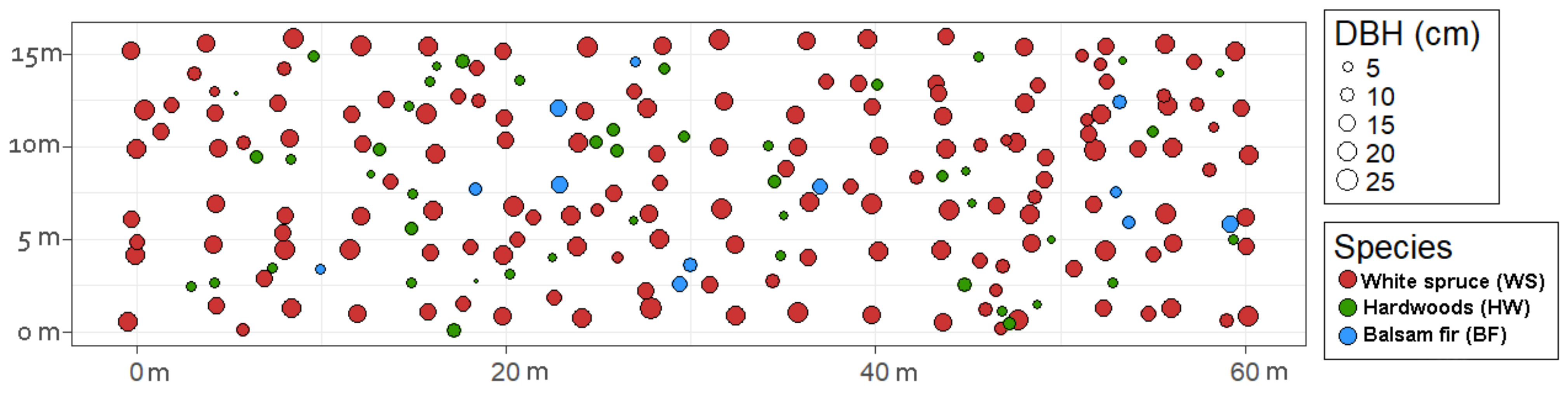
2.2. Data Acquisition

Considering the large area of the plots, the quantity of trees to be positioned, and the difficulty of manually positioning them, the use of terrestrial lidar was preferred to obtain the most precise spatial coordinates of all trees (including saplings). Terrestrial lidar is a powerful technology for capturing the three-dimensional structure of forests with a high level of precision [42,43]. All plots were scanned immediately after treatment with a Faro^® Focus 3D terrestrial laser scanner (TLS). Thirteen scans were done per plot to obtain full plot coverage and to minimise occlusion. Spherical targets (at least 3 seen from each scan position) were placed throughout the plot and used for scan registration. These multiple scans were then aligned to create a single 3-dimensional point cloud with the Faro^® Scene 5.0 software (FARO Technologies, Rugby, Warwickshire, UK).

We used the point cloud to map the coordinates of each tree in each plot (Figure 1). To do so, we imported the point clouds in the R programming environment [44]. We produced a digital terrain model from the points with the lowest altitude and reconstructed the ground surface with a Delaunay triangulation using the lidR package [45]. Then, we extracted a 20 cm slice of points centred at 1.30 m above the ground. To eliminate returns due to the branches, the 20 cm slice was rasterised on the XY plan into 1 × 1 cm rasters. We took advantage of the fact that rasters with points from a stem have a higher density than those with branches to derive a threshold for cleaning the data from raster that did not contain stems. The remaining points were clustered using density-based algorithms implemented in the DBSCAN package [46]. Finally, we automatically adjusted a circle to the points in the cluster to measure the diameter at breast height (DBH; measured at 1.3 m) and to obtain the XY coordinates of all the trees with a DBH greater than 1 cm. We corrected some DBH mis-adjustments (e.g., to add missing trees or delete clusters not belonging to trees) following a manual visual validation. Since no efficient algorithms to recognise species via TLS were available, species were conventionally tallied and then merged into 3 groups (Gsp): white spruce (WS), balsam fir (BF), and merchantable hardwoods (HW). The HW group included paper birch, yellow birch, sugar maple, red maple, ash (Fraxinus sp.), and trembling aspen. Some rare species (e.g., eastern white cedar, Thuja occidentalis L.) and non-commercial hardwoods (e.g., elderberry (Sambucus nigra ssp. canadensis (L.) R. Bolli), rowan (Sorbus aucuparia L.), and speckled alder (Alnus incana ssp. rugosa (Du Roi) R.T. Clausen)) were not considered in the analysis.

A total of 10,696 trees were kept for the analysis. In order to deal with border effects, we used all border trees (i.e., those located within 1.5 m of the plot edges) as neighbours to calculate the distances between neighbours. These distances were also used to calculate the Clark and Evans index [6,47] (Equation (1)), which describes the aggregation of trees at the stand level. This index was calculated for each Gsp (R_WS, R_BF, and R_HW) and all trees (including saplings and merchantable trees) (

Table 1. Mean characteristics (minimum–maximum) of stands by treatment for all commercial species (total), white spruce, balsam fir, and hardwoods.

		TrT0 (Control)				TrTCT (Crop Tree Release Thinning)
		Total	White Spruce	Balsam Fir	Hardwoods	Total	White Spruce	Balsam Fir	Hardwoods
Quadratic diameter (cm)	All trees	15.1 [11.8–17.2]	15.5 [13.3–17.5]	14.0 [8.8–21.6]	8.5 [5.5–13.5]	15.4 [13.4–18.4]	15.8 [14.2–18.2]	15.2 [7.8–22.9]	8.0 [5.3–10.8]
	Saplings	6.4 [4.8–7.6]	6.7 [5.5–7.5]	5.9 [3.6–8.0]	5.3 [3.7–7.0]	7.0 [5.2–7.9]	7.2 [5.5–8.4]	6.4 [2.1–8.7]	6.0 [4.2–7.7]
	Merchantable trees	16.8 [14.8–17.8]	16.7 [14.9–18.1]	16.3 [12.4–21.6]	14.5 [9.8–22.9]	16.6 [15.0–19.0]	16.4 [15.1–18.6]	17.6 [10.4–22.9]	12.6 [9.2–16.0]
Stand density (trees per ha)	All trees	2247 [1544–3134]	1719 [951–2283]	360 [94–1054]	168 [0–886]	1994 [1166–2754]	1524 [827–2270]	377 [42–1317]	93 [0–497]
	Saplings	537 [121–1715]	301 [55–714]	105 [0–219]	131 [0–781]	344 [67–801]	164 [28–333]	106 [0–532]	74 [0–436]
	Merchantable trees	1702 [1364–2161]	1418 [806–2007]	255 [54–909]	37 [0–159]	1649 [1082–2098]	1360 [785–1937]	270 [21–785]	19 [0–121]
Stand basal area (m2 per ha)	All trees	39.1 [34–45.4]	32.0 [17.7–42.9]	6.1 [0.9–24.7]	0.9 [0.0–5.3]	36.5 [29.1–44.0]	29.2 [20.5–38.5]	6.8 [0.4–21.0]	0.5 [0.0–2.5]
	Saplings	1.5 [0.4–3.1]	1.0 [0.2–1.8]	0.3 [0.0–0.8]	0.2 [0.0–1.0]	1.3 [0.3–2.4]	0.7 [0.1–1.4]	0.4 [0.0–2.0]	0.2 [0.0–1.2]
	Merchantable trees	37.7 [31.1–44.9]	31.1 [17.2–42.3]	5.9 [0.8–24.2]	0.7 [0.0–4.3]	35.3 [27.2–42.6]	28.5 [20–37.1]	6.5 [0.2–20.9]	0.3 [0.0–1.7]
Clark and Evans aggregation index	All trees	1.23 [1.03–1.50]	1.34 [1.18–1.56]	0.90 [0.32–1.48]	0.94 [0.67–1.48]	1.32 [1.03–1.49]	1.36 [1.17–1.60]	0.93 [0.50–1.46]	0.74 [0.37–0.92]
	Saplings	1.02 [0.83–1.19]	0.99 [0.82–1.34]	0.96 [0.55–1.28]	0.85 [0.69–0.95]	1.00 [0.26–1.52]	1.16 [0.88–1.35]	1.00 [0.32–1.42]	0.77 [0.43–1.02]
	Merchantable trees	1.34 [1.19–1.51]	1.34 [1.17–1.54]	0.91 [0.51–1.34]	1.05 [0.65–1.46]	1.35 [1.14–1.52]	1.34 [1.14–1.57]	0.94 [0.47–1.48]	1.25 [0.70–1.74]
		TrT1/3 (Thinning From Below)				TrTBF (all Balsam Fir Trees are Harvested)
		Total	White Spruce	Balsam Fir	Hardwoods	Total	White Spruce	Balsam Fir	Hardwoods
Quadratic diameter (cm)	All trees	15.8 [13.5–19.9]	16.0 [14.3–18.5]	16.4 [8.6–24.6]	9.0 [5.6–13.2]	14.3 [11.5–15.6]	14.8 [14–15.8]	13.1 [1.2–23.7]	11.4 [5.2–39.1]
	Saplings	6.3 [5.0–7.5]	6.5 [5.5–7.7]	5.9 [4.4–7.2]	5.0 [3.5–7.9]	5.9 [5.5–7.0]	6.3 [5.5–7.4]	4.5 [1.2–8.4]	4.8 [2.2–6.7]
	Merchantable trees	17.2 [14.9–20.9]	17.0 [14.8–19.2]	18.6 [10.5–24.6]	14.9 [11.6–23.5]	16.4 [14.7–18.2]	16.3 [15.0–18.0]	17.4 [14.1–23.7]	19.0 [11.7–47.8]
Stand density (trees per ha)	All trees	1706 [1040–2585]	1345 [631–2178]	219 [0–1066]	141 [0–635]	2254 [1313–3892]	1809 [1053–2237]	106 [11–271]	339 [9–1662]
	Saplings	341 [49–889]	181 [0–489]	55 [0–406]	105 [0–508]	657 [226–1755]	334 [200–458]	39 [0–109]	284 [9–1445]
	Merchantable trees	1365 [686–2159]	1164 [580–2017]	165 [0–660]	36 [0–127]	1597 [890–2137]	1475 [749–1900]	67 [0–219]	55 [0–217]
Stand basal area (m2 per ha)	All trees	31.9 [19.5–46.2]	26.2 [16.5–38.6]	4.8 [0.0–15.0]	0.9 [0.0–5.0]	34.6 [24.3–40.5]	31.2 [17.1–36.4]	1.6 [0.0–5.4]	1.7 [0.0–5.3]
	Saplings	1.0 [0.1–2.0]	0.6 [0.0–1.5]	0.2 [0.0–1.5]	0.2 [0.0–0.9]	1.6 [0.9–4.1]	1.0 [0.7–1.5]	0.1 [0.0–0.4]	0.5 [0.0–2.8]
	Merchantable trees	30.9 [18.4–45]	25.6 [16.3–37.5]	4.6 [0.0–15.0]	0.7 [0.0–4.5]	33.1 [23.1–36.4]	30.2 [16.4–35.2]	1.6 [0.0–5.3]	1.2 [0.0–3.9]
Clark and Evans aggregation index	All trees	1.26 [1.00–1.55]	1.33 [0.98–1.60]	0.96 [0.67–1.33	0.77 [0.51–1.35]	1.22 [1.11–1.45]	1.31 [1.09–1.52]	0.74 [0.52–0.83]	0.72 [0.51–0.90]
	Saplings	1.08 [0.68–1.56]	1.14 [0.95–1.39]	1.04 [0.64–1.51]	0.76 [0.46–0.90]	0.92 [0.74–1.13]	1.05 [0.87–1.24]	0.92 [0.27–1.44]	0.68 [0.43–0.90]
	Merchantable trees	1.34 [1.02–1.55]	1.32 [1.04–1.60]	1.02 [0.69–1.33]	1.17 [0.34–2.33]	1.30 [1.10–1.49]	1.30 [1.01–1.50]	0.83 [0.48–1.25]	1.03 [0.82–1.13]

). A value below 1 indicated a tendency to cluster, a value close to 1 as associated with a random distribution, and a value above 1 indicated a regular distribution.

$${\mathrm{R}}_{\mathrm{Gsp}}=\frac{{\mathrm{R}}_{\mathrm{obs}}}{{\mathrm{R}}_{\mathrm{theo}}} \mathrm{with}\sim \left\{\begin{array}{l}{\mathrm{R}}_{\mathrm{obs}}=\frac{{{\displaystyle \sum }}_{\mathrm{i}=1}^{\mathrm{N}}{\mathrm{r}}_{\mathrm{i}}}{\mathrm{N}}\hfill \\ {\mathrm{R}}_{\mathrm{theo}}=\frac{1}{2\sqrt{\frac{\mathrm{N}}{\mathrm{Area}}}}\hfill \end{array}\right.$$

(1)

where N represents the number of trees for a given Gsp and r_i is the distance between tree i and its closest neighbour of the same Gsp.

Stand characteristics are summarized in Table 1. The variables used in this study and their abbreviations are listed in

Table 2. Definition and abbreviation of the variables used.

Category	Variable	Description
Plot-level	TrT	General notation of the sylvicultural treatment affecting the stand
	TrT0	Control (no treatment)
	TrTBF	Thinning with priority selection of balsam fir, in which all the balsam fir are harvested
	TrT1/3	Thinning from below, in which the smallest trees are cut while ensuring equal spacing between the remaining trees
	TrTCT	Crop tree release thinning to remove competition 3 m around a selected number of crop trees on observed data (from 0 to 4.5 m on simulated data)
	Gsp	General group notation for trees being regrouped by species (WS, BF, HW, or total)
	WS	Group containing all white spruce (Picea glauca) trees
	BF	Group containing all balsam fir (Abies balsamea) trees
	HW	Group containing all commercial hardwood species (described in text)
	Tot	Group containing all the trees from WS, BF, and HW
	NHaGsp	Tree density per hectare for a given Gsp
	RGsp	Aggregation index for a given Gsp
Species-level	NClusHaGsp	Number of clusters per hectare for a given Gsp (calculated using the affinity propagation clustering method)
	DistBF	Closest distance between 2 BF trees inside a cluster
	DistHW	Closest distance between 2 HW trees inside a cluster
Tree-level	T0	Target tree (i.e., tree to be positioned)
	T1	Closest competitor tree to T0
	T2	Second closest competitor tree to T0
	DBHDiff	Absolute difference in diameter at breast height between T0 and T1
	MinDistComp	Closest distance between two trees (where Competitor can be T1 or T2)

.

2.3. Modelling Spatial Stand Structure

We used a spatial distribution simulator to describe the spatial stand structure in WS plantations. This simulator includes models at the tree level describing intra- and interspecific interactions between neighbouring trees. These models are presented in the following paragraphs.

For each model developed in this study, we tested a list of potential stand-level explanatory variables including silvicultural treatment, aggregation index, and stand density, as well as potential tree-level variables including DBH, Gsp, and interactions between them. Variables that were highly correlated were excluded (variance inflation factor (VIF) > 10 [48]).

We used the glm stats library of the R statistical programming environment [44] to fit the models, and we selected variables using a backward elimination process based on the corrected form of Akaike’s information criterion (AICc) [49].

2.3.1. Clark and Evans index

At the stand level, spatial structure can be summarised by the Clark and Evans index, which provides a single value by Gsp following a linear model (Equation (2)).

$${\mathrm{R}}_{\mathrm{Gsp}}=\mathrm{X}\mathsf{\omega }+\mathsf{\epsilon }$$

(2)

where $\mathrm{X}$ is the design matrix of covariates, ω is the fixed-effect parameter vector to be estimated, and ε is the error term.

2.3.2. Spatial Interactions between Individual Trees

At the individual tree level, spatial structure was characterised on the basis of interactions between neighbouring trees. We calculated the distance between a tree and its neighbours by a nearest neighbour analysis using the RANN package [50], from which we obtained the distance to the 2 closest neighbours (MinDist_T1 and MinDist_T2). Then, we modelled these 2 distances as a function of the available inventory stand variables and of those from the targeted tree and its 2 nearest neighbours. As these distances are continuous and positive variables, we used a gamma regression model [51] (Equation (3)).

$$\mathrm{Y}={\mathrm{e}}^{\mathrm{Z}\mathsf{\gamma }}+\mathsf{\epsilon }$$

(3)

where Y is the distance to a neighbour (MinDistT1 or MinDistT2), $\mathrm{Z}$ is the design matrices of covariates, γ is the fixed-effect parameter vector to be estimated, and ε is the error term.

2.3.3. Spatial Interactions within Species Groups

For Gsp with a R_Gsp ≥ 1, no intraspecific interaction was modelled. However, for those Gsp that tended to form clusters (R_Gsp < 1), we first determined the number of clusters observed in a stand using the method of affinity propagation clustering [52] (Figure 2).

To describe these aggregations, we characterised 2 variables: the number of clusters per Gsp per hectare (NClusHa_Gsp) and the distance between trees of the same Gsp within a cluster. As NClusHa_Gsp is a count variable (positive and discrete), we chose a Poisson regression model [51]. The general model equation form was similar to Equation (3), where Y is the number of clusters per hectare and per Gsp (NClusHa_Gsp), $\mathrm{Z}$ is the covariate design matrix, and γ the fixed effect parameter vector to be estimated.

Within a cluster, we computed the minimal distance between a tree and its closest neighbour of the same Gsp (Dist_Gsp). We calculated this distance by a nearest neighbour analysis using the RANN package [50]. Since Dist_Gsp is a continuous and positive variable, A gamma regression was choose to model Dist_Gsp [51].

2.3.4. Model Validation

We used a repeated 5-fold cross validation to calculate the predictive accuracy of the models [53]. The stands were randomly split into 5 subsets of equal size: the first four were used to calibrate the model, and the fifth was used to validate it. The root mean square error (RMSE) and the determination coefficient (R²) of the predictions were then calculated using the validation subset. The process was repeated until all subsets were used to validate the model. The random segregation of the plots into the subsets was repeated 50 times. The validation result was the average of all the repetitions.

2.4. Spatial Stand Structure Simulation

2.4.1. Spatial Stand Structure Generator

After building these models, we developed a spatial stand structure generator (hereafter referred to as a “spatialiser”) to generate coordinates for a non-spatial inventory. This “spatialiser” generates random coordinates that are evaluated to determine if positioning is possible based on the inter- and intraspecies models presented above. To avoid edge effects (i.e., trees close to the plot border having no competitors on the exterior side), the simulated plot has to be embedded in a torus in order to keep the same plot area and have no border effects. We followed these steps to generate a list of XY coordinates for each tree:

• Trees were ordered by DBH.
• For the Gsp where R_Gsp < 1, the number of clusters (NClusHa_Gsp) was calculated.
• For all trees, we repeated the following steps, depending on Gsp.
  • For trees with R_Gsp ≥ 1, we generated a random position, identified the 2 closest competitors and, knowing the characteristics (Gsp and DBH) of the neighbours, calculated the theoretical minimum distance with these 2 trees (i.e., MinDist_T1 and MinDist_T2). If the 2 measured distances were greater than the 2 theoretical values, the point was kept as a potential valid position.
  • For trees with R_Gsp < 1, if the number of trees of the same Gsp already positioned was less than the predicted NClusHa_Gsp, the tree was positioned randomly. If the number of trees of the same Gsp was greater than NClusHa_Gsp, we randomly selected a tree of the same Gsp that was already positioned and used it as an anchor for a cluster. From this anchor position, we generated a random point around the anchor point at a distance equal to the modelled Dist_Gsp. Finally, this position was then evaluated in the same way as in the previous point, i.e., by comparing the distances between the target tree and the 2 closest neighbours.
• The generator could start from an empty stand. However, a plantation scheme describing the spacing between planted trees and the presence of planting rows could be used to place planted trees species in these positions. A thinning path could also be added.

2.4.2. Performance Tests of the “Spatialiser”

In order to assess the effectiveness of the “spatialiser” to generate a realistic spatial stand structure, we selected the 15 control plots from the dataset, simulated the tree coordinates with the “spatialiser,” and then calculated the Clark and Evans index for each Gsp.

We also simulated the same plots by assigning random coordinates to the trees (i.e., by not considering the interactions between trees). Hence, we simulated the 15 control plots in both methods (“spatialiser” vs. random) and calculated the Clark and Evans index for each Gsp and both simulations. These simulations were repeated 100 times.

Afterward, we performed an ANOVA to evaluate the difference between the index of the 2 simulations (random vs. “spatialiser”). As a final step, we calculated the bias between observed index and simulated index values.

2.4.3. Thinning Treatment Simulations

As TrT_CT, TrT_1/3, and TrT_BF were used as independent variables in the models, the “spatialiser” could directly simulate a recently thinned stand with one of these 3 thinning treatments. However, the main use of the “spatialiser” (once it was integrated into the growth model) was to simulate a realistic spatial tree distribution in WS plantations where a thinning treatment could be applied. The applied treatment could be like those used in this study or of another type.

To illustrate this application, we chose 2 interventions. The first was the TrT_CT thinning treatment already used in this study. The second was the creation of gaps. Gaps are carried out operationally in certain cutblocks in eastern Quebec to create openings for wildlife. The 2 selected treatments create openings in the stand that can promote regeneration by seed trees, as well as recreate other stand attributes such structural diversity. As skidding trails are an essential component of commercial thinning operations, they were added to both simulations (about 33 m apart and 4 m wide).

The first treatment (TrT_CT) aims to free the selected dominant trees from competition. This treatment is the first step of a series of interventions aimed at changing the silviculture path from even-aged to uneven-aged stands. It is characterized by two parameters: the number of selected crop trees (50–100/ha) and the thinning radius around each tree (1–5 m). We randomly selected the thinned trees among those of merchantable size within the stand, with the only requirement being that 2 selected trees had to be at least 9 m apart.

The second treatment (Gap creation) aims to create larger openings in the stand canopy in order to promote regeneration in the opening [54]. We performed this gap simulation to evaluate the behaviour of the spatial model for a treatment in which the choices of the number of gaps, their position in the stand, and their size are very important. In these simulations, the gap positions were chosen randomly. However, in an operational context, their choice should depend on the proximity of selected seed trees, the autecology of the species to be regenerated, the autecology of competing or harmful species, and the position of the skidding trails. The number of gaps varies from 1 to 4, and total gap area varies from 5% and 40% of the total stand area (i.e., 500–4000 m²).

To simulate the effect of these 2 treatments, we selected 15 un-thinned stands (TrT₀) in which we upscaled plot size to 1 hectare and positioned all trees with the “spatialiser.” We then applied both treatments and calculated the Clark and Evans index for each Gsp in these simulated plots. For each treatment, the simulation was repeated 100 times. We performed an ANOVA to compare the means of the different groups obtained after the simulations and to assess the impact of the treatment parameters on the spatial distribution (i.e., the number of selected crop trees and thinning radius around each tree for TrT_CT and the number of gaps and total percentage of surface cut for gap creation).

3. Results

3.1. Modelling Spatial Stand Structure

3.1.1. Clark and Evans Index

The spatial distribution of WS tended to be regular (R_WS = 1.34; Figure 3 and

Table 3. Parameters estimations (standard error) of the model selected to predict aggregation index at the stand level (Equation (4)) (* (p < 0.05); ** (p < 0.001); *** (p < 0.0001)).

Coefficient	Variable †	RGsp
a0	(Intercept)	1.69069	(0.18456)	***
a1	NHaGsp	0.00022	(0.00007)	**
a2	NHatot	−0.00030	(0.00007)	***
a3	BF	−0.04347	(0.11409)
	HW	−0.12414	(0.11901)
a4	TrTCT	−0.47603	(0.23238)	*
	TrT1/3	−0.44839	(0.19339)	*
	TrTBF	−0.91933	(0.23554)	***
a5	BF: NHaGsp	−0.00030	(0.00011)	**
	HW: NHaGsp	−0.00031	(0.00013)	*
a6	TrTCT: NHatot	0.00020	(0.00010)
	TrT1/3: NHatot	0.00017	(0.00009)
	TrTBF: NHatot	0.00034	(0.00010)	***

^† See Table 2 for variable definitions.

), which was expected, given that the stands were plantations. Conversely, BF and HW tended to form clusters, with HW following a stronger trend (R_BF = 0.92 and R_HW = 0.79; Figure 3). The final model form for predicting the aggregation index was found to be:

$$\begin{array}{cc}\hfill {\mathrm{R}}_{\mathrm{Gsp}}=& {\mathrm{a}}_0+{\mathrm{a}}_1\times {\mathrm{NHa}}_{\mathrm{Gsp}}+{\mathrm{a}}_2\times {\mathrm{NHa}}_{\mathrm{tot}}+{\mathrm{a}}_3\times \mathrm{Gsp}+{\mathrm{a}}_4\times \mathrm{TrT}+\hfill \\ \hfill & {\mathrm{a}}_5\times {\mathrm{NHa}}_{\mathrm{Gsp}}\times \mathrm{Gsp}+{\mathrm{a}}_6\times {\mathrm{NHa}}_{\mathrm{tot}}\times \mathrm{TrT}+\mathsf{\epsilon }\hfill \end{array}$$

(4)

where a₀–a₆ are the parameter estimates for the fixed effects found in Table 3.

Fit statistics show that the proportion of total variation explained by the model (R²) was 0.84 and that the RMSE was 0.12. The RMSE and R² were 0.08 and 0.65 for R_WS, 0.15 and 0.58 for R_BF, and 0.14 and 0.64 for R_HW, respectively.

For each species, the Clark and Evans index value was inversely proportional to the total stand density (a₂ = −0.00030; Table 3). At the species level, R_WS was proportional to WS tree density (a₁ = 0.00022), whereas R_BF and R_HW were inversely proportional to BF and HW density (a₅ = −0.00030 for BF and −0.00031 for HW). On average and compared to the control plots, commercial thinning slightly decreased the aggregation index value, making a regular distribution more random and a random distribution more aggregated. The strongest effect was for TrT_BF (a₄ = −0.91933), followed by TrT_CT (a₄ = −0.47603), and TrT_1/3 (a₄ = −0.44839. However, for TrT_BF, the aggregation index significantly increased with total density (a₆ = 0.00034).

3.1.2. Spatial Interactions between Individual Trees

The final model form for MinDist_T1 (the distance between a target tree and the first competitor) is presented in Equation (5) (R² = 0.38 and RMSE = 0.49).

$${\log (\mathrm{MinDist}}_{\mathrm{T}1}{)=\mathrm{b}}_0{+\mathrm{b}}_1{\times \mathrm{R}}_{\mathrm{Gsp}}{+\mathrm{b}}_2{\times \mathrm{DBH}}_{\mathrm{T}0}{+\mathrm{b}}_3{\times \mathrm{Gsp}}_{\mathrm{T}0}{+\mathrm{b}}_4{\times \mathrm{DBH}}_{\mathrm{T}1}{+\mathrm{b}}_5{\times \mathrm{Gsp}}_{\mathrm{T}1}{+\mathrm{b}}_6{\times \mathrm{NHa}}_{\mathrm{Gsp}}{+\mathrm{b}}_7{\times \mathrm{NHa}}_{\mathrm{tot}}+\mathsf{\epsilon }$$

(5)

where b₀–b₇ are the parameter estimates for the fixed effects found in

Table 4. Parameters estimations (standard error) of the models selected to predict the distance of the two nearest competitors (Equations (5) and (6)) (* (p < 0.05); ** (p < 0.001); *** (p < 0.0001)).

Coefficient	Variable †	MinDistT1			MinDistT2
b0	(Intercept)	−0.46104	(0.04497)	***	0.11132	(0.03626)	**
b1	RGsp	0.60337	(0.03083)	***	0.36470	(0.02402)	***
b2	DBHT0	0.00018	(0.00001)	***	0.00012	(0.00001)	***
b3	BFT0	−0.07628	(0.02564)	**	−0.09724	(0.01971)	***
	HWT0	−0.22557	(0.02938)	***	−0.17750	(0.02261)	***
b4	DBHT1	0.00015	(0.00001)	***	0.00010	(0.00001)	***
b5	BFT1	−0.19511	(0.01360)	***	−0.10188	(0.01071)	***
	HWT1	−0.27708	(0.01469)	***	−0.15679	(0.01151)	***
b6	NHaGsp	−0.00008	(0.00002)	***	−0.00011	(0.00001)	***
b7	NHatot	−0.00011	(0.00001)	***	−0.00007	(0.00001)	***
b8	DBHT2				0.00007	(0.00001)	***
b9	BFT2				−0.08173	(0.01148)	***
	HWT2				−0.11974	(0.01253)	***
b10	TrTCT				0.02701	(0.00948)	**
	TrT1/3				0.04731	(0.00964)	***
	TrTBF				0.01166	(0.00979)

^† See Table 2 for variable definitions.

.

We observed that the minimum distance between the target trees and the first competitor increased with the aggregation index (b₁ = 0.60337; Table 4) and with the DBH of the target tree and its closest neighbour (T0: b₂ = 0.00018 and T1: b₄ = 0.00015). The distance was smaller for HW or BF, and the effect was greater for HW (T0: b₃ = −0.22557 and T1: b₅ = −0.27708). The greater the total density and the density of trees of the same Gsp as the target tree, the smaller the distance (NHa_Gsp: b₆ = −0.00008 and NHa_tot: b₇ = −0.00011).

The final model form for MinDist_T2 (the distance between a target tree and the second-closest competitor) is presented in Equation (6) (R² = 0.32 and RMSE = 0.56).

$$\begin{array}{cc}\hfill {\log (\mathrm{MinDist}}_{\mathrm{T}2})=& {\mathrm{b}}_0{+\mathrm{b}}_1{\times \mathrm{R}}_{\mathrm{Gsp}}{+\mathrm{b}}_2{\times \mathrm{DBH}}_{\mathrm{T}0}{+\mathrm{b}}_3{\times \mathrm{Gsp}}_{\mathrm{T}0}{+\mathrm{b}}_4{\times \mathrm{DBH}}_{\mathrm{T}1}{+\mathrm{b}}_5{\times \mathrm{Gsp}}_{\mathrm{T}1}{+\mathrm{b}}_6{\times \mathrm{NHa}}_{\mathrm{Gsp}}{+\mathrm{b}}_7{\times \mathrm{NHa}}_{\mathrm{tot}}\hfill \\ & +{\mathrm{b}}_8{\times \mathrm{DBH}}_{\mathrm{T}2}{+\mathrm{b}}_9{\times \mathrm{Gsp}}_{\mathrm{T}2}{+\mathrm{b}}_{10}\times \mathrm{TrT}+\mathsf{\epsilon }\hfill \end{array}$$

(6)

where b₀–b₁₀ are the parameter estimates for the fixed effects found in Table 4.

Similar results to MinDist_T1 were observed for MinDist_T2 (Table 4), except that this distance was also positively influenced by the DBH_T2 of the second competitor (b₈ = 0.00007) and negatively influenced when T2 was part of the HW or BF Gsp, with a more important effect for HW (T2: b₉ = −0.11974). In addition, the TrT_1/3 and TrT_CT thinning treatments both increased MinDist_T2 (TrT_1/3: b₁₀ = 0.04731 and TrT_CT: b₁₀ = 0.02701).

3.1.3. Spatial Interactions within Species Groups

As R_WS was superior to 1, we only modelled intraspecific interaction for BF and HW. The number of clusters per hectare and per species was predicted by Equation (7) (R² = 0.41, RMSE = 1.7):

$$\log \left({\mathrm{NClusHa}}_{\mathrm{Gsp}}\right)={\mathrm{c}}_0+{\mathrm{c}}_1\times \mathrm{Gsp}+{\mathrm{c}}_8\times \mathrm{TrT}+{\mathrm{c}}_{11}\times \mathrm{Gsp}\times \mathrm{TrT}+\mathsf{\epsilon }$$

(7)

where c₀, c₁, c₈, and c₁₁ are the parameter estimates for the fixed effects found in

Table 5. Parameters estimations (standard error) of the models selected to predict intra-species spatial distribution (Equations (7)–(9)). (* p < 0.05; ** p < 0.001; *** p < 0.0001).

Coefficient	Variable †	NClusHaGsp			DistBF			DistHW
c0	(Intercept)	3.56105	(0.07538)	***	0.49974	(0.10200)	***	0.85028	(0.31248)	**
c1	HW	0.42423	(0.09695)	***
c2	DBHDiff				0.00113	(0.00041)	**
c3	DBHT0							0.00287	(0.00066)	***
c4	DBHT1				0.00109	(0.00031)	***	0.00215	(0.00070)	*
c5	R				0.94840	(0.09473)	***	1.24419	(0.16511)	***
c6	NHaGsp				−0.00107	(0.00006)	***	−0.00279	(0.00039)	***
c7	NHatot							−0.00022	(0.00011)	*
c8	TrTCT	−0.14880	(0.12912)		0.04792	(0.05024)
	TrT1/3	−0.31400	(0.10601)	**	0.12117	(0.05391)	*
	TrTBF	−0.12706	(0.10144)		0.16893	(0.07865)	*
c9	DBHT0: DBHT1							−0.00002	(0.00001)	*
c10	NHatot: NHaGsp							5.6e-07	(0.00000)	***
c11	HW: TrTCT	0.15866	(0.16286)
	HW: TrT1/3	0.32693	(0.13133)	*
	HW: TrTBF	0.32710	(0.12721)	*

^† See Table 2 for variable definitions.

.

The number of clusters per hectare was greater for HW (c₁ = 0.42423; Table 5), with an average value of 30 clusters for BF and 57 for HW for all treatments. TrT_1/3 was the only thinning treatment that significantly reduced the number of clusters (c₈ = −0.31400) compared to the control treatment, but this was only for BF, since the interaction between HW and TrT_1/3 (c₁₁ = 0.32693) negated this effect for HW. The interaction HW with TrT_BF (c₁₁ = −0.32710), for its part, indicated that there were more HW clusters in this treatment than in the control.

The shape parameters of the gamma distribution for minimal distance between trees of the same species within a cluster were 1.204 for BF and 0.959 for HW, while the scale parameters were 0.357 for BF and 0.403 for HW. For BF, the final model for predicting the minimal distance is presented in Equation (8) (R² = 0.19, RMSE = 3.22):

$$\log \left({\mathrm{Dist}}_{\mathrm{BF}}\right)={\mathrm{c}}_0+{\mathrm{c}}_2\times {\mathrm{DBH}}_{\mathrm{diff}}+{\mathrm{c}}_4\times {\mathrm{DBH}}_{\mathrm{T}1}+{\mathrm{c}}_5\times {\mathrm{R}}_{\mathrm{Gsp}}+{\mathrm{c}}_6\times {\mathrm{NHa}}_{\mathrm{Gsp}}+{\mathrm{c}}_8\times \mathrm{TrT}+\mathsf{\epsilon }$$

(8)

where c₀, c₂, c₄, c₅, c₆, and c₈ are the parameter estimates for the fixed effects found in Table 5.

The final model is slightly different for HW (Equation (9), R² = 0.25, RMSE = 2.39):

$$\begin{array}{cc}\hfill \log \left({\mathrm{Dist}}_{\mathrm{HW}}\right)={\mathrm{c}}_0& +{\mathrm{c}}_3\times {\mathrm{DBH}}_{\mathrm{T}0}+{\mathrm{c}}_4\times {\mathrm{DBH}}_{\mathrm{T}1}+{\mathrm{c}}_5\times {\mathrm{R}}_{\mathrm{Gsp}}+{\mathrm{c}}_6\times {\mathrm{NHa}}_{\mathrm{Gsp}}+{\mathrm{c}}_7\times {\mathrm{NHa}}_{\mathrm{tot}}+{\mathrm{c}}_9\times {\mathrm{DBH}}_{\mathrm{T}0}\times {\mathrm{DBH}}_{\mathrm{T}1}+{\mathrm{c}}_{10}\hfill \\ & \times {\mathrm{NHa}}_{\mathrm{Gsp}}{\mathrm{NHa}}_{\mathrm{tot}}+ \mathsf{\epsilon }\hfill \end{array}$$

(9)

where c₀, c₃, c₄, c₅, c₆, c₇, c₉, and c₁₀ are the parameter estimates for the fixed effects found in Table 5.

Inside a cluster, the distance between two trees of the same species increased as the DBH of the closest neighbour increased (c₄ = 0.00109 for BF and c₄ = 0.00215 for HW; Table 5). The DBH of the target tree also had a positive effect for HW (c₃ = 0.00287). For BF, the larger the difference in DBH between two neighbour trees, the larger the distance between the two trees (c₂ = 0.00113), whereas for HW, the higher the DBH_T0:DBH_T1 ratio, the shorter the distance between the two trees (c₉ = −0.00002). The distance between two trees of the same Gsp was smaller when the density of the Gsp was high (c₆ = −0.00107 for BF and c₆ = −0.00279 for HW). For HW, this distance was also reduced in stands with a high density (c₇ = −0.00022).

For BF, the TrT_1/3 and TrT_BF treatments increased the minimal distance between two trees compared to the control (c₈ = 0.12117 for TtT_1/3 and 0.16893 for TrT_BF; Table 5).

3.2. Spatial Stand Structure Simulation

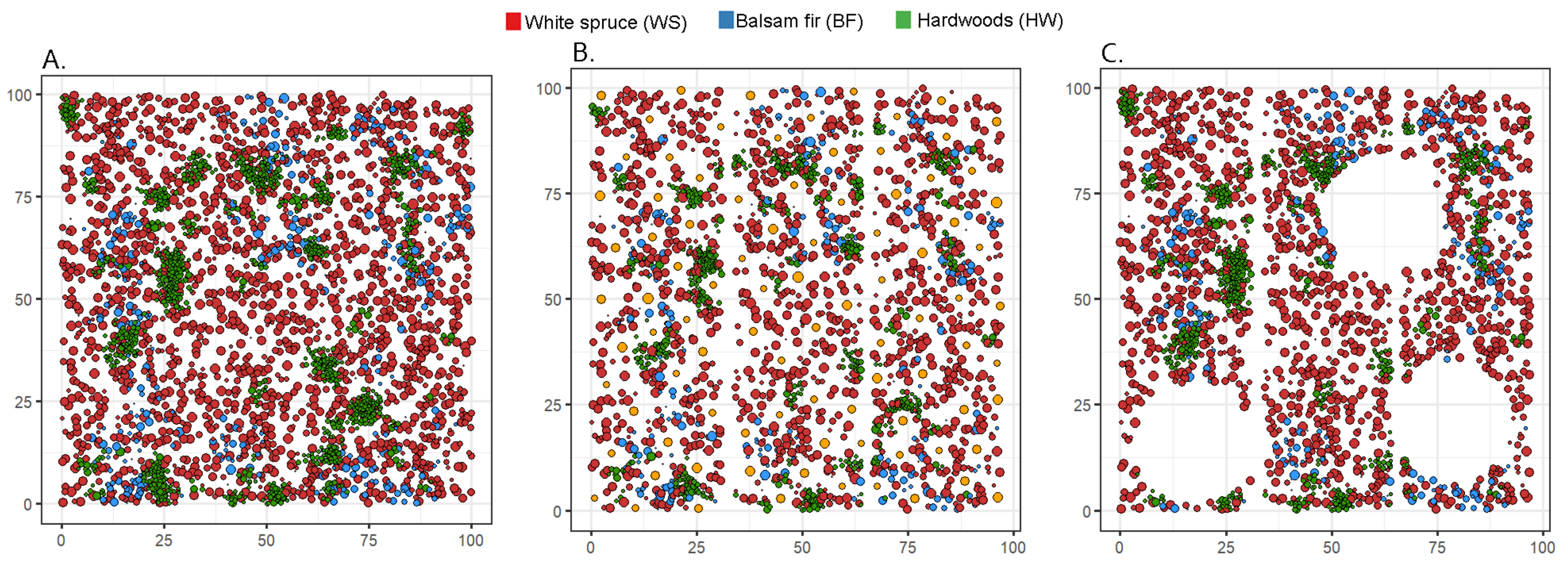
3.2.1. Performance Tests of the “Spatialiser”

Based on the Clark and Evans index calculated after the simulations, we observed that the “spatialiser” worked better than randomly assigning coordinates to trees to generate a realistic spatial stand distribution (Figure 4). We measured the correlation and bias between observed and simulated data. On average, for the “spatialiser,” R² was 0.63 and RMSE was 0.19, whereas for the random simulations, R² was 0.01 and RMSE was 0.30. However, we observed disparities between Gsp (Figure 4). For WS, R² was 0.29 and RMSE was 0.18 with the “spatialiser,” (R² = 0.01 and RMSE = 0.36 for the random simulations); for BF, R² was 0.28 and RMSE was 0.18 with the “spatialiser” (R² = 0.02 and RMSE = 0.31 for the random simulations). For HW, R² was 0.69 and RMSE was 0.21 with the “spatialiser” (R² = 0.10 and RMSE = 0.43 for the random simulations).

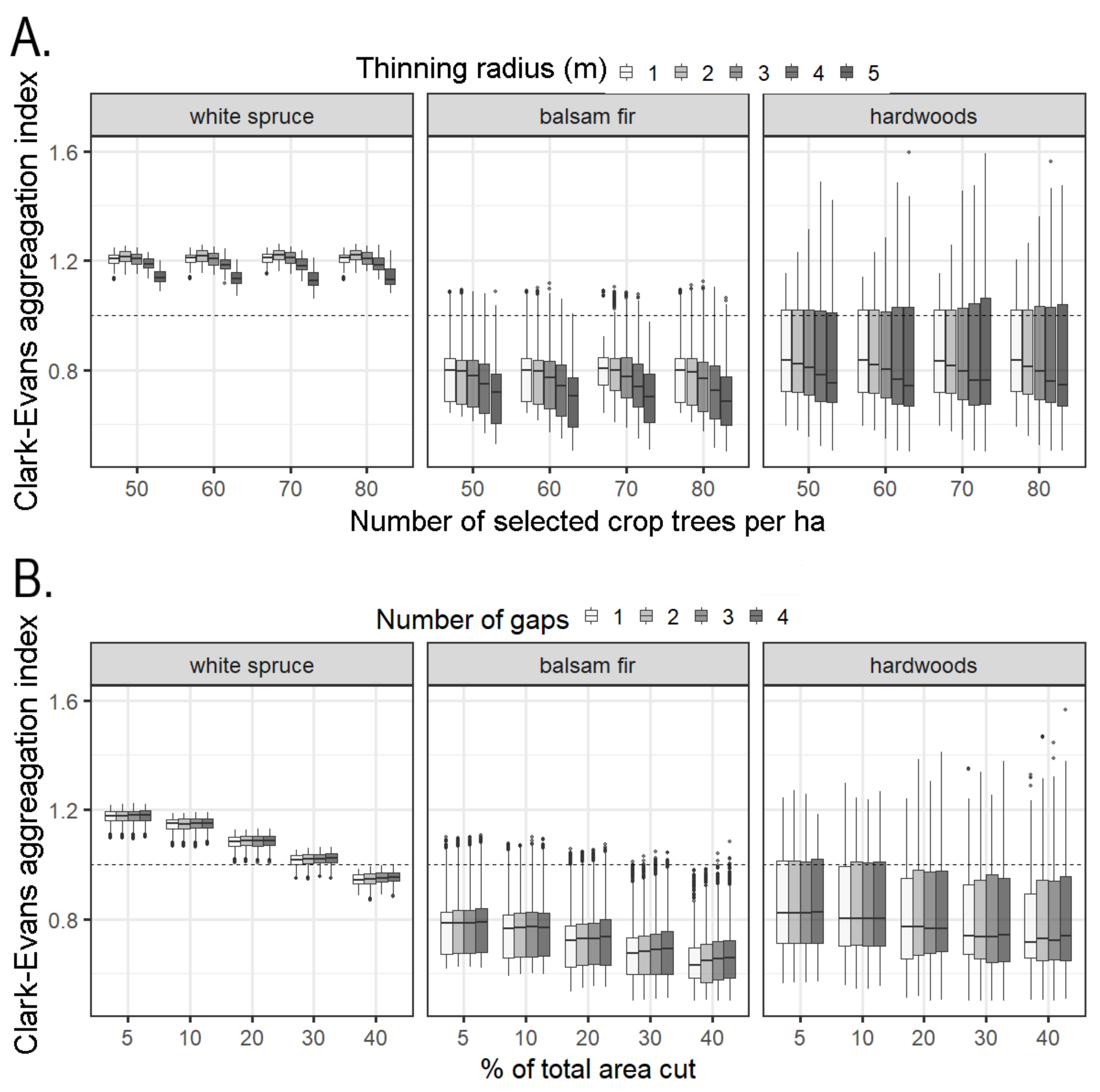
3.2.2. Thinning Treatment Simulations

Figure 5 presents the results of one simulation over a 1-hectare area before treatment and after applying either the TrT_CT or gap creation treatment.

With the TrT_CT treatment, an increase of the thinning radius around each tree and the number of trees freed from competition significantly affected the aggregation index value. The link between the aggregation index and these two parameters was negative, except in WS, for which there were slight positive effects on the number of crop trees (R_WS = 0.0001 for the number of crop trees and −0.0158 for thinning radius, R_BF = −0.0004 for the number of crop trees and −0.0026 for thinning radius, and R_HW = −0.0002 for the number of crop trees and −0.0136 for thinning radius). These negative parameters indicated that greater treatment intensity decreased the aggregation index value. However, the effect on spatial structure at the stand level was very limited (Figure 6A).

With gap creation treatment, increases in both the number of gaps and the total percentage of the area that was cut had significant effects on the aggregation index value. The link was positive with the number of gaps but negative with the percentage of the surface cut (R_WS = 0.0001 for the number of crop trees and −0.6415 for the percentage of surface cut, R_BF = 0.0044 for the number of crop trees and −0.3965 for the percentage of surface cut, and R_HW = 0.0040 for the number of crop trees and −0.3049 for the percentage of surface cut). Despite its significance, the effect of the number of gaps was found to be very small at the stand scale. By comparison, increasing the cut surface had a much greater effect on stand spatial structure, especially for WS (Figure 6B).

4. Discussion

4.1. Modelling Spatial Stand Structure

A stand’s spatial structure results from interactions between trees; it is one of the most important ecological characteristics influencing its development. In plantations, human actions such as (initial spacing and thinning) can be added and modify these processes. The model we developed describes local intra- and interspecific interactions and links point patterns with ecological/silvicultural processes. Despite the absence of precise biological information such as crown characteristics, which are known to strongly influence the behaviour between two closely located trees, it was possible to develop a “spatialiser” that can reproduce attractive behaviours among trees of the same species and repulsive behaviours among trees that are too close. Choi et al. [55] showed that adding more detailed competition variables provided only slightly better predictions of spatial patterns for hardwoods. In addition, in most situations where data are limited to standard inventories (e.g., species, DBH, and height), the “spatialiser” would need to rely on allometric relationships to predict the needed crown attributes [56]. This would generate a source of uncertainty and error propagation. Hence, coupling a “spatialiser” to standard inventory data could be an interesting alternative to measuring the location of trees in the field and would allow for the use of models working with spatially explicit plantation growth simulators. The spatial information could also be used to calculate structural habitat characteristics and shed light on the stand community structure and relative abundance of animal species [57].

Some limitations and simplifications of this spatial simulator should be considered. The models were calibrated on plantations that have less complex structures than natural stands, even if plantations in eastern Quebec have a high proportion of regeneration by other species [58]. In addition, we chose to group all the different hardwood species together and to remove some species of coniferous very rarely present as well as non-commercial species from the analysis. These species, however, could have a significant effect on competition or be of great interest to understand the diversity of species. Additionally, saplings and merchant trees were studied together. However, saplings are generally present in large numbers, whereas merchant trees are the result of competition over a longer term. These differences could be reflected in the spatial distribution of these two groups (Table 1). However, despite these limitations, the combination of tree-scale models considering DBH and species of neighbouring trees, as well as a plot-scale model describing the type of aggregation of a species, seems flexible enough to adapt to different types of stands.

4.2. Spatial Interactions between Individual Trees

The construction of the “spatialiser” using several models has the advantage of allowing for a direct interpretation of inter- and intraspecific interactions. At the stand level, the Clark and Evans aggregation index (R) [47] showed that in the studied plantations, WS had a regular structure while BF and HW tended to aggregate. For the planted WS seedlings, this was expected. However, for the WS saplings that were naturally established later on, the structure was more aggregated (Table 1). The Clark and Evans index that was chosen here is a simple and easy to measure variable for analysing the spatial behaviour of a species at the plot scale. The simulator models were of the tree scale. The unique value of the index then allowed us to simply assess the results of the simulation at the plot level. In order to apply the simulation approach to other types of stands with more species involved or used as surrogate measures to quantify biodiversity, some other indexes could be used to describe or validate the stand spatial structure [59].

The grouping of hardwood species in our analysis prevented us from examining the behaviour of each individual hardwood species. Some of these, such as paper birch, tended to aggregate. In the case of aspen, vegetative reproduction by suckering could explain its tendency to group [10]. Other species, such as red maple and sugar maple, appear to be less aggregated, although red maple can form clusters in cases where it forms stump sprouts [60]. Both BF and HW tended to aggregate; however, the observed clusters were different. For BF, clusters were fewer, but they tended to include both merchantable-sized trees and saplings. For HW, clusters were smaller, more numerous, and consisted mainly of saplings.

Currently, in the Bas-Saint-Laurent region, natural stands are mainly dominated by BF and HW, to the detriment of WS [58]. In plantations, BF and HW can represent up to 25% of the trees. In order to limit competition and to favour the growth of WS, a species that is becoming rarefied [34], good knowledge regarding this species’ spatial behaviour and natural regeneration, as well as the development of competing species, is needed. The tendency to BF and HW to cluster can help managers choose approaches that limit their spread to the detriment of WS when they prescribe clearing, precommercial thinning, or commercial thinning treatments.

4.3. Thinning Treatment Simulations

At the tree level, species and DBH were the most important parameters influencing the distribution of BF and HW. At the stand scale, however, thinning caused only slight changes in the aggregation index, except for TrT_BF. This was normal, because the purpose of these treatments was to reduce competition in order to increase mean tree wood production. In addition, TrT_CT could be considered as a first step to convert plantation structure from regular/even-aged to irregular/uneven-aged if the objective is to reduce the differences between natural and managed forests [61]. However, after five years, this treatment had no significant effect on diameter distribution or spatial structure. Dupont-Leduc [61] suggested that a five-year interval is probably too short to observe such differences. The lack of structural change may also suggest that the thinning intensity of the TrT_CT treatment was not sufficient or too evenly applied [61]. Indeed, for the two other thinning treatments, cuts were only done around 50–100 dominant trees with a clearance limited between 2.5 and 3 m (TrT_CT) or mainly with the aim of promoting dominated trees (TrT_1/3). Nevertheless, TrT_CT could also allow for the long-term development of seed trees and thus the maintenance of WS rather than its replacement by BF. Though it is unclear whether the small observed differences in stand structure compared to the control will be conserved or will evolve in time, the reduction of the number of trees per hectare and of competition could help trees to grow faster and create more heterogeneous forests. Gauthier et al. [62] showed that with a TrT_1/3 thinning, stand structural heterogeneity increased 10 years after the harvest as a result of the better growth of bigger trees and retention of saplings. However, according to Schütz [29], many entries are necessary for the conversion effect to become apparent from regular/even-aged stands to irregular/uneven-aged stands. Thus, several years of stand monitoring will be required to evaluate the real long-term impact of these anthropic disturbances [63].

The “spatialiser” can be used to generate control stands with localised trees where “silvicultural“ treatments can be simulated. This would allow for the evaluation of the chosen approach’s effectiveness and the testing of silvicultural treatments [64]. Such an exercise suggests that, for example, TrT_CT could be applied with a larger clearance distance around targeted trees, since simulations showed that the current TrT_CT treatment had a fairly limited impact and that a rather large clearance around trees was needed to modify the spatial distribution at the stand scale. Hence, to emulate natural disturbances, the treatment should create larger gaps. According to the simulations, the creation of larger gaps (e.g., cut area: 5–40% of the total) could be another effective approach to modify stand spatial structure. However, for both these examples, the thinning effect was observed directly after application. An evaluation of the long-term effectiveness of the chosen approach is also required. To do this, the “spatialiser” could be harnessed for a growth model and help forecast evolution at both the individual tree and stand scales.

5. Conclusions

This study shows that the spatial structure of WS plantations in eastern Quebec, Canada can be modelled and simulated. The diameter and species of the neighbour trees were the most important factors that explained the observed distances between trees. A point process model proved effective at representing inter-tree interactions through repulsive and attractive processes. Analysing all hardwood species in a single group limits the understanding of each species’ spatial behaviour. However, since BF and hardwoods together could represent 30–40% of a stand’s basal area, the models allow for the better understanding of their interactions with WS.

Our results showed that thinning treatments can have slightly significant and short-term effects on spatial structure. If the objective is to convert to another stand structure type, linking this “spatialiser” to growth models would allow for the simulation of treatments over larger areas and longer periods. It would also allow for parameters to be modified in order to evaluate the effectiveness of the chosen approach. Thus, silvicultural treatments could be adjusted to better reach management objectives.

References

1. Batista, J.L.F.; Maguire, D.A. Modelling the spatial structure of tropical forests. For. Ecol. Manag. 1998, 110, 293–314. [Google Scholar] [CrossRef]
2. Pommerening, A.; Stoyan, D. Reconstructing spatial tree point patterns from nearest neighbour summary statistics measured in small subwindows. Can. J. For. Res. 2008, 38, 1110–1122. [Google Scholar] [CrossRef] [Green Version]
3. Weiskittel, A.R.; Hann, D.W.; Kershaw, J.A.; Vanclay, J.K. Forest Growth and Yield Modelling; John Wiley & Sons: Chichester, UK, 2011; ISBN 9781119998518. [Google Scholar]
4. Vanclay, J.K. Modelling Forest Growth and Yield: Applications to Mixed Tropical Forests; CAB International: Wallingford, UK, 1994; p. 537. [Google Scholar]
5. Pommerening, A. Evaluating structural indices by reversing forest structural analysis. For. Ecol. Manag. 2006, 224, 266–277. [Google Scholar] [CrossRef]
6. Pretzsch, H. Analysis and modeling of spatial stand structures. Methodological considerations based on mixed beech-larch stands in Lower Saxony. For. Ecol. Manag. 1997, 97, 237–253. [Google Scholar] [CrossRef]
7. Lim, K.; Treitz, P.; Wulder, M.; St-Onge, B.; Flood, M. LiDAR remote sensing of forest structure. Prog. Phys. Geogr. 2003, 27, 88–106. [Google Scholar] [CrossRef] [Green Version]
8. Pacala, S.W.; Deutschman, D.H. Details That Matter: The Spatial Distribution of Individual Trees Maintains Forest Ecosystem Function. Oikos 2017, 74, 357–365. [Google Scholar] [CrossRef]
9. Law, R.; Illian, J.; Burslem, D.F.R.P.; Gratzer, G.; Gunatilleke, C.V.S.; Gunatilleke, I. Ecological information from spatial patterns of plants: Insights from point process theory. J. Ecol. 2009, 97, 616–628. [Google Scholar] [CrossRef]
10. Bärring, U. On the reproduction of aspen (Populus tremula L.) with emphasis on its suckering ability. Scand. J. For. Res. 1988, 3, 229–240. [Google Scholar] [CrossRef]
11. Hibbs, D.E.; Fischer, B.C. Sexual and vegetative reproduction of striped maple (Acer pensylvanicum L.). Bull. Torrey Bot. Club 1979, 106, 222–227. [Google Scholar] [CrossRef]
12. Koop, H. Vegetative reproduction of trees in some European natural forests. Vegetatio 1987, 72, 103–110. [Google Scholar] [CrossRef]
13. Gray, A.N.; Spies, T.A. Microsite controls on tree seedling establishment in conifer forest canopy gaps. Ecology 1997, 78, 2458–2473. [Google Scholar] [CrossRef]
14. Yamamoto, S.-I. Forest gap dynamics and tree regeneration. J. For. Res. 2000, 5, 223–229. [Google Scholar] [CrossRef]
15. Wiegand, T.; Moloney, K.A. Handbook of Spatial Point-Pattern Analysis in Ecology; CRC: Boca Raton, FL, USA, 2013; ISBN 1420082558. [Google Scholar]
16. Diggle, P.J. Statistical Analysis of Spatial and Spatio-Temporal Point Patterns; CRC: Boca Raton, FL, USA, 2013; ISBN 146656024X. [Google Scholar]
17. Fortin, M.; Dale, M.R.T.; Ver Hoef, J.M. Spatial analysis in ecology. Wiley StatsRef Stat. Ref. Online 2014. [Google Scholar] [CrossRef]
18. Genet, A.; Grabarnik, P.; Sekretenko, O.; Pothier, D. Incorporating the mechanisms underlying inter-tree competition into a random point process model to improve spatial tree pattern analysis in forestry. Ecol. Model. 2014, 288, 143–154. [Google Scholar] [CrossRef]
19. Diggle, P.J.; Fiksel, T.; Grabarnik, P.; Ogata, Y.; Stoyan, D.; Tanemura, M. On parameter estimation for pairwise interaction point processes. Int. Stat. Rev. 1994, 62, 99–117. [Google Scholar] [CrossRef]
20. Grabarnik, P.; Särkkä, A. Interacting neighbour point processes: Some models for clustering. J. Stat. Comput. Simul. 2001, 68, 103–125. [Google Scholar] [CrossRef]
21. Obiang, N.L.E.; Ngomanda, A.; Mboma, R.; Nzabi, T.; Ngoye, A.; Atsima, L.; Ndjélé, L.; Mate, J.; Lomba, C.; Picard, N. Spatial pattern of central African rainforests can be predicted from average tree size. Oikos 2010, 119, 1643–1653. [Google Scholar] [CrossRef]
22. Grabarnik, P.; Särkkä, A. Modelling the spatial and space-time structure of forest stands: How to model asymmetric interaction between neighbouring trees. Procedia Environ. Sci. 2011, 7, 62–67. [Google Scholar] [CrossRef] [Green Version]
23. Franklin, J.F.; Van Pelt, R. Remote sensing of structural complexity indices for habitat and species distribution modeling. J. For. 2004, 3, 22–28. [Google Scholar]
24. Estes, L.D.; Reillo, P.R.; Mwangi, A.G.; Okin, G.S.; Shugart, H.H. Remote sensing of structural complexity indices for habitat and species distribution modeling. Remote Sens. Environ. 2010, 4, 792–804. [Google Scholar] [CrossRef]
25. Gouvernement du Québec. Du Loi sur L’Aménagement Durable du Territoire Forestier; Gouvernement du Québec: Quebec, QC, Canada, 2015.
26. Gauthier, S.; Vaillancourt, M.-A.; Leduc, A.; De Grandpré, L.; Kneeshaw, D.; Morin, H.; Drapeau, P.; Bergeron, Y. Ecosystem Management in the Boreal Forest; Presses de l’Université du Québec: Québec, QC, Canada, 2009; ISBN 2760523829. [Google Scholar]
27. Harvey, B.D.; Leduc, A.; Gauthier, S.; Bergeron, Y. Stand-landscape integration in natural disturbance-based management of the southern boreal forest. For. Ecol. Manag. 2002, 155, 369–385. [Google Scholar] [CrossRef]
28. Franklin, J.F.; Mitchell, R.J.; Palik, B. Natural Disturbance and Stand Development Principles for Ecological Forestry; US Department of Agriculture: Washington, DC, USA, 2007.
29. Schütz, J. Silvicultural tools to develop irregular and diverse forest structures. Forestry 2002, 75, 329–337. [Google Scholar] [CrossRef] [Green Version]
30. Ruel, J.-C.; Roy, V.; Lussier, J.-M.; Pothier, D.; Meek, P.; Fortin, D. Mise au point d’une sylviculture adaptée à la forêt boréale irrégulière. For. Chron. 2007, 83, 367–374. [Google Scholar] [CrossRef] [Green Version]
31. Boucher, Y.; Arseneault, D.; Sirois, L.; Blais, L. Logging pattern and landscape changes over the last century at the boreal and deciduous forest transition in Eastern Canada. Landsc. Ecol. 2009, 24, 171–184. [Google Scholar] [CrossRef]
32. Dupuis, S.; Arseneault, D.; Sirois, L. Change from pre-settlement to present-day forest composition reconstructed from early land survey records in eastern Québec, Canada. J. Veg. Sci. 2011, 22, 564–575. [Google Scholar] [CrossRef]
33. Boucher, Y.; Arseneault, D.; Sirois, L. Logging-induced change (1930–2002) of a preindustrial landscape at the northern range limit of northern hardwoods, eastern Canada. Can. J. For. Res. 2006, 36, 505–517. [Google Scholar] [CrossRef] [Green Version]
34. Grondin, P.; Cimon, A. Les Enjeux de Biodiversité Relatifs à la Composition Forestière; Gouvernement du Québec, Ministère des Ressources Naturelles, de la Faune et des Parcs: Quebec, QC, Canada, 2003.
35. Eriksson, S.; Hammer, M. The challenge of combining timber production and biodiversity conservation for long-term ecosystem functioning—A case study of Swedish boreal forestry. For. Ecol. Manag. 2006, 237, 208–217. [Google Scholar] [CrossRef]
36. O’Hara, K.L. The historical development of uneven-aged silviculture in North America. Forestry 2002, 75, 339–346. [Google Scholar] [CrossRef]
37. Pretzsch, H. Transitioning Monocultures to Complex Forest Stands in Central Europe: Principles and Practice; Burleigh Dodds Science Publishing Limited: Cambridge, UK, 2019. [Google Scholar]
38. Schütz, J.-P. Opportunities and strategies of transforming regular forests to irregular forests. For. Ecol. Manag. 2001, 151, 87–94. [Google Scholar] [CrossRef]
39. Robitaille, A.; Saucier, J.-P. Forestiers, Québec (Province). Direction de la gestion des stocks; [Québec]. In Paysages Régionaux Du Québec Méridional; Gouvernement du Québec, Ministère des Ressources naturelles: Quebec, QC, Canada, 1998. [Google Scholar]
40. Grondin, F.; Drouin, N. Optitek Sawmill Simulator-User’s Guide; Forintek Canada Corporation: Québec, QC, Canada, 1998. [Google Scholar]
41. Gagné, L.; Sirois, L.; Lavoie, L. Comparaison du volume et de la valeur des bois résineux issus d’éclaircies par le bas et par dégagement d’arbres-élites dans l’Est du Canada. Can. J. For. Res. 2016, 11, 1320–1329. [Google Scholar] [CrossRef] [Green Version]
42. Dassot, M.; Constant, T.; Fournier, M. The use of terrestrial LiDAR technology in forest science: Application fields, benefits and challenges. Ann. For. Sci. 2011, 68, 959–974. [Google Scholar] [CrossRef] [Green Version]
43. Trochta, J.; Krůček, M.; Vrška, T.; Král, K. 3D Forest: An application for descriptions of three-dimensional forest structures using terrestrial LiDAR. PLoS ONE 2017, 12, e0176871. [Google Scholar] [CrossRef] [PubMed] [Green Version]
44. R Core Team. R: A Language and Environment for Statistical Computing; R Foundation for Statistical Computing: Vienna, Austria, 2019. [Google Scholar]
45. Roussel, J.R.; Auty, D.; Coops, N.C.; Tompalski, P.; Goodbody, T.R.H.; Sánchez Meador, A.; Bourdon, J.F.; De Boissieu, F.; Achim, A. lidR: An R package for analysis of Airborne Laser Scanning (ALS) data. Remote Sens. Environ. 2020, 251, 112061. [Google Scholar] [CrossRef]
46. Hahsler, M.; Piekenbrock, M.; Arya, S.; Mount, D. dbscan: Density Based Clustering of Applications with Noise (DBSCAN) and Related Algorithms. R Package Version. 2019. Available online: https://CRAN.R-project.org/package=dbscan (accessed on 28 May 2021).
47. Clark, P.J.; Evans, F.C. Distance to nearest neighbour as a measure of spatial relationships in populations. Ecology 1954, 35, 445–453. [Google Scholar] [CrossRef]
48. O’brien, R.M. A Caution Regarding Rules of Thumb for Variance Inflation Factors. Qual. Quant. 2007, 41, 673–690. [Google Scholar] [CrossRef]
49. Burnham, K.P.; Anderson, D.R. Model Selection and Multimodel Inference: A Practical Information-Theoretic Approach; Springer: Berlin/Heidelberg, Germany, 2002; Volume 172, p. 488. [Google Scholar]
50. Arya, S.; Mount, D.; Kemp, S.E.; Jefferis, G. RANN: Fast Nearest Neighbour Search (Wraps ANN Library) Using L2 Metric. R Package Version 2.6.1. 2019. Available online: https://CRAN.R-project.org/package=RANN (accessed on 28 May 2021).
51. Faraway, J.J. Extending the Linear Model with R: Generalized Linear, Mixed Effects and Nonparametric Regression Models; CRC Press: Boca Raton, FL, USA, 2016; Volume 124, ISBN 1498720986. [Google Scholar]
52. Frey, B.J. Clustering by passing messages between data points. Science 2007, 315, 972–976. [Google Scholar] [CrossRef] [Green Version]
53. Rodriguez, J.D.; Perez, A.; Lozano, J.A. Sensitivity Analysis of k-Fold Cross Validation in Prediction Error Estimation. IEEE Trans. Pattern Anal. Mach. Intell. 2010, 32, 569–575. [Google Scholar] [CrossRef]
54. Coates, K.D. Tree recruitment in gaps of various size, clearcuts and undisturbed mixed forest of interior British Columbia, Canada. For. Ecol. Manag. 2002, 155, 387–398. [Google Scholar] [CrossRef]
55. Choi, J.; Lorimer, C.G.; Vanderwerker, J.; Cole, W.G.; Martin, G.L. A crown model for simulating long-term stand and gap dynamics in northern hardwood forests. For. Ecol. Manag. 2001, 152, 235–258. [Google Scholar] [CrossRef]
56. Schneider, R.; Berninger, F.; Ung, C.H.; Bernier, P.Y.; Swift, D.E.; Zhang, S.Y. Calibrating jack pine allometric relationships with simultaneous regressions. Can. J. For. Res. 2008, 38, 2566–2578. [Google Scholar] [CrossRef]
57. St-Laurent, M.H.; Ferron, J.; Hins, C.; Gagnon, R. Effects of stand structure and landscape characteristics on habitat use by birds and small mammals in managed boreal forest of eastern Canada. Can. J. For. Res. 2007, 37, 1298–1309. [Google Scholar] [CrossRef]
58. Duchateau, E.; Schneider, R.; Tremblay, S.; Dupont-Leduc, L. Density and diameter distributions of saplings in naturally regenerated and planted coniferous stands in Quebec after various approaches of commercial thinning. Ann. For. Sci. 2020, 77, 38. [Google Scholar] [CrossRef]
59. Pommerening, A. Approaches to quantifying forest structures. Forestry 2002, 75, 305–324. [Google Scholar] [CrossRef]
60. Wilson, B.F. Red Maple Stump Sprouts: Development the First Year; Harvard University: Harvard, MA, USA, 1968; Volume 10. [Google Scholar]
61. Dupont-Leduc, L.; Schneider, R.; Sirois, L. Preliminary results from a structural conversion thinning trial in Eastern Canada. J. For. 2020, 118, 515–533. [Google Scholar] [CrossRef]
62. Gauthier, M.-M.; Barrette, M.; Tremblay, S. Commercial thinning to meet wood production objectives and develop structural heterogeneity: A case study in the spruce-fir forest, Quebec, Canada. Forests 2015, 6, 510–532. [Google Scholar] [CrossRef]
63. Pretzsch, H. Diversity and productivity in forests: Evidence from long-term experimental plots. In Forest Diversity and Function; Springer: Berlin/Heidelberg, Germany, 2005; pp. 41–64. ISBN 3540221913. [Google Scholar]
64. Greene, D.F.; Kneeshaw, D.D.; Messier, C.; Lieffers, V.; Cormier, D.; Doucet, R.; Coates, K.D.; Groot, A.; Grover, G.; Calogeropoulos, C. Modelling silvicultural alternatives for conifer regeneration in boreal mixedwood stands (aspen/white spruce/balsam fir). For. Chron. 2002, 78, 281–295. [Google Scholar] [CrossRef] [Green Version]
Figure 1. Tree map of the 3 groups of species for one of the 900 m2 plots of the second experiment.
Forests 12 00740 g001
Figure 2. Example of intraspecific clustering throughout a stand for (A) balsam fir and (B) hardwoods. All the trees within a given cluster are connected by a set of lines of the same colour. The coloured surface was added afterward to facilitate the viewing of clusters.
Forests 12 00740 g002
Figure 3. Box plots of observed (dark grey bars) and predicted (light grey bars) values of the Clark and Evans aggregation index, by species group (Gsp) and silvicultural treatment, for all trees. See Table 2 for definitions of Gsp and treatment abbreviations.
Forests 12 00740 g003
Figure 4. Comparison between Clark and Evans indexes observed for the 3 species groups (Gsp: see Table 2 for definitions) and the indexes predicted from the “spatialiser” simulations and from random simulations.
Forests 12 00740 g004
Figure 5. Example of simulations on a 1-hectare area for (A) initial spatial stand structure; (B) TrTCT: 80 crop trees (orange dots) selected per hectare, with a 3 m thinning radius over all sides; and (C) gap creation (3 gaps; cut area: 30% of the total). The vertical spaces visible on plots (B,C) are skidding trails, which essential for commercial thinning operations.
Forests 12 00740 g005
Figure 6. Variation of the Clark and Evans aggregation index for each species group (Gsp) after simulating (A) the number of crop trees selected per hectare, with various clearance distances (thinning radii) around each tree, and (B) the proportion of the total area that was cut, with a variable number of gaps. See Table 2 for definitions of Gsp and treatment abbreviations.
Forests 12 00740 g006