Author Contributions
Conceptualization, P.C. and D.K.; methodology, P.C., D.K., I.L., and B.H.; software, P.C.; validation, P.C.; formal analysis, P.C.; investigation, P.C. and D.K.; resources, P.C., D.K., and I.L.; data curation, P.C.; writing—original draft preparation, P.C.; writing—review and editing, P.C., D.K., I.L., and B.H.; visualization, P.C.; supervision, D.K.; project administration, P.C. and D.K.; funding acquisition, P.C., D.K., and I.L. All authors have read and agreed to the published version of the manuscript.
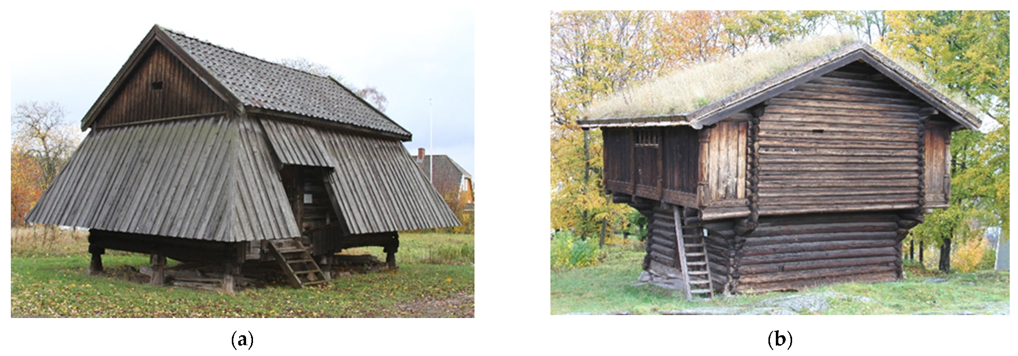
Figure 1.
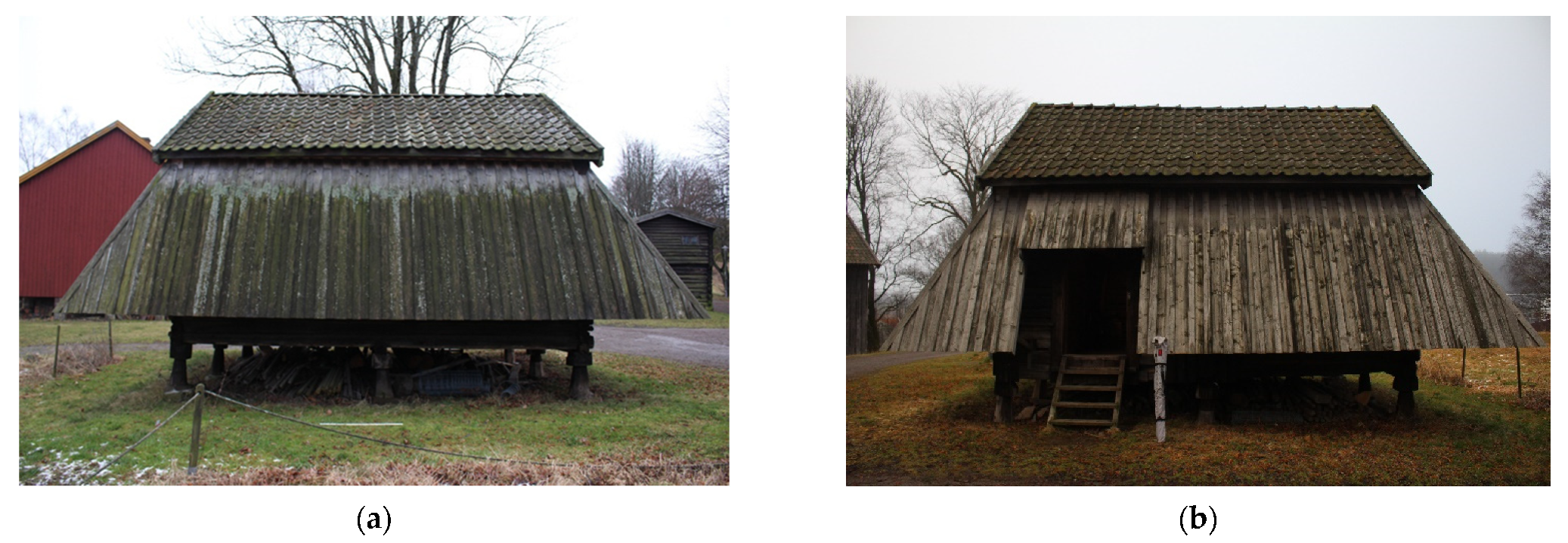
Photographs of (a) the Fadum storehouse and (b) the Heierstad loft taken from south-west.
Figure 1.
Photographs of (a) the Fadum storehouse and (b) the Heierstad loft taken from south-west.
Figure 2.
The building components have been grouped in four homogeneous categories, highlighted with different colors, based on the type and age of wood that they are made of. The positions of the installed sensors are also highlighted with green color for the air temperature and humidity sensors (A, C, F, G, I, K), blue color for the moisture content sensors (B, D, H, J), and red color for the sensor monitoring the temperature inside the timber (E).
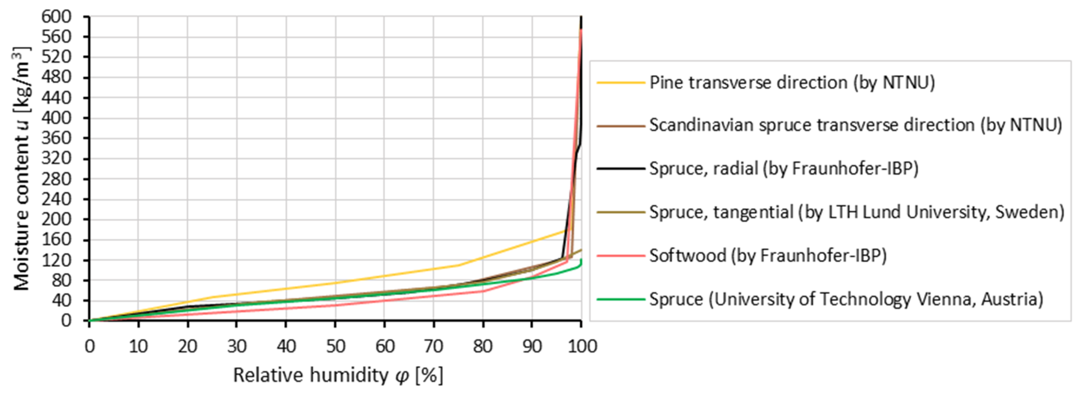
Figure 3.
Moisture storage functions of the wood species that were tested for the selection of proper material properties for the two case studies. The data derive from the WUFI® database.
Figure 3.
Moisture storage functions of the wood species that were tested for the selection of proper material properties for the two case studies. The data derive from the WUFI® database.
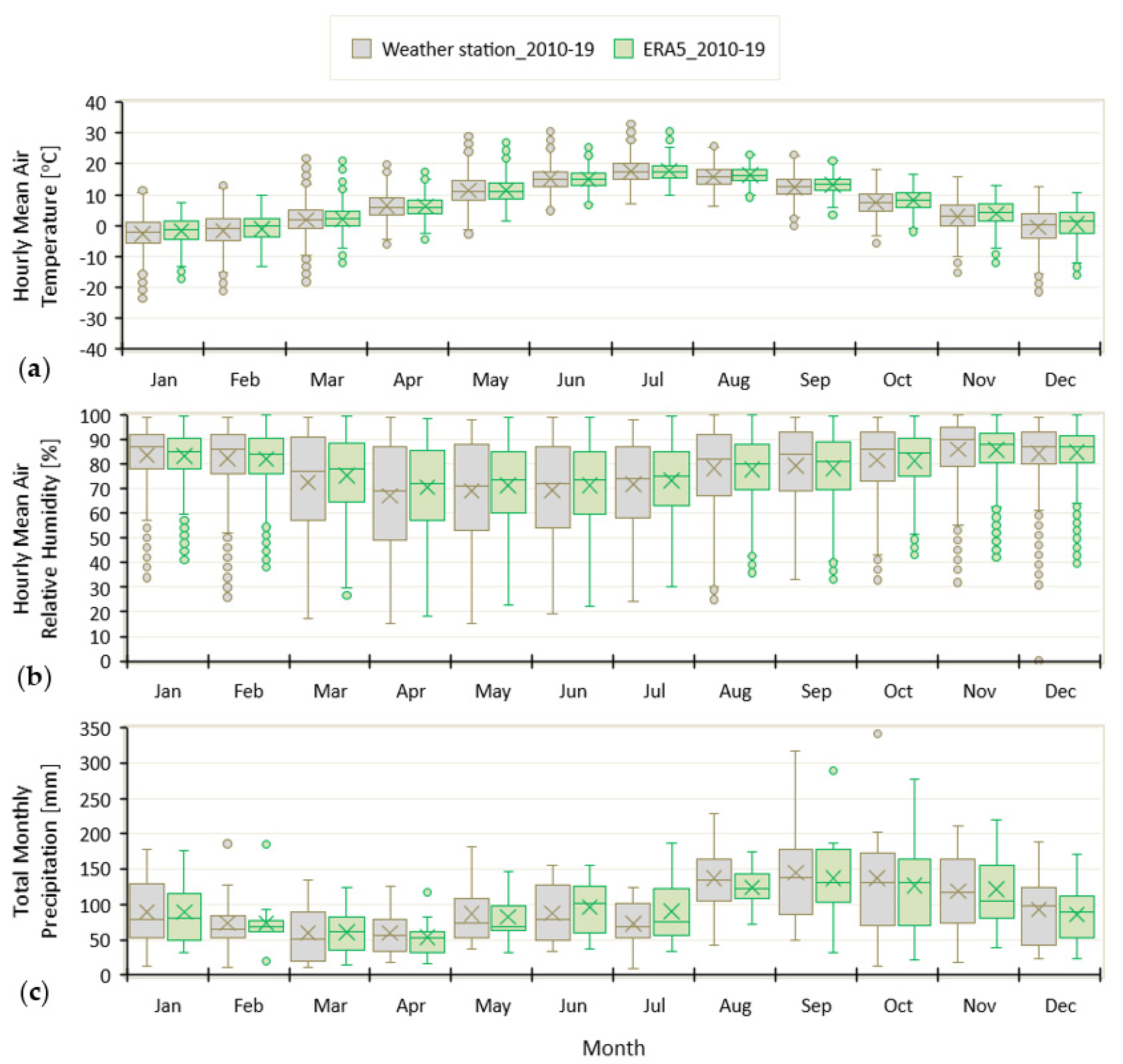
Figure 4.
Comparison between (a) air temperature, (b) air relative humidity and (c) precipitation data derived from the Melsom weather station that is located 5 km from the study site, and from the ERA5 reanalysis. In the boxplots the box shows 50% of the data, with median represented as a horizontal bar and the average value highlighted with the ‘x’ symbol. The whisker extends to two standard deviations of the data and the circles represent the outliers.
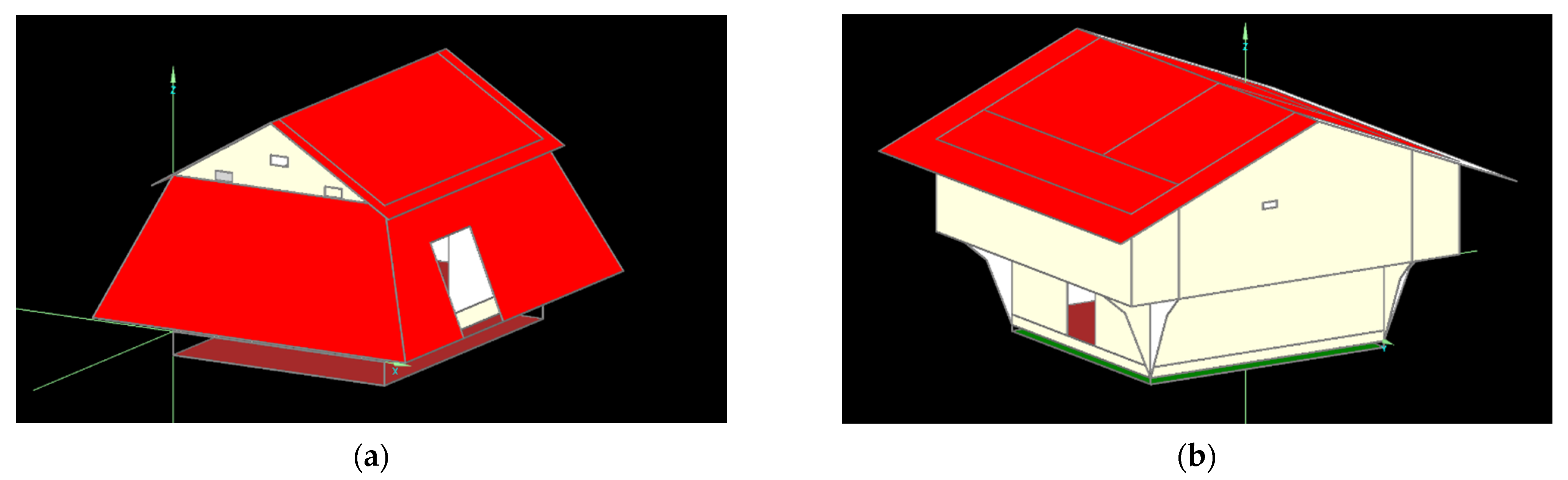
Figure 5.
The whole-building simulation models of (a) the Fadum storehouse and (b) the Heierstad loft.
Figure 5.
The whole-building simulation models of (a) the Fadum storehouse and (b) the Heierstad loft.
Figure 6.
At the Fadum storehouse, the growth of biological organisms is more intense on (a) the north façade than on (b) the south façade.
Figure 6.
At the Fadum storehouse, the growth of biological organisms is more intense on (a) the north façade than on (b) the south façade.
Figure 7.
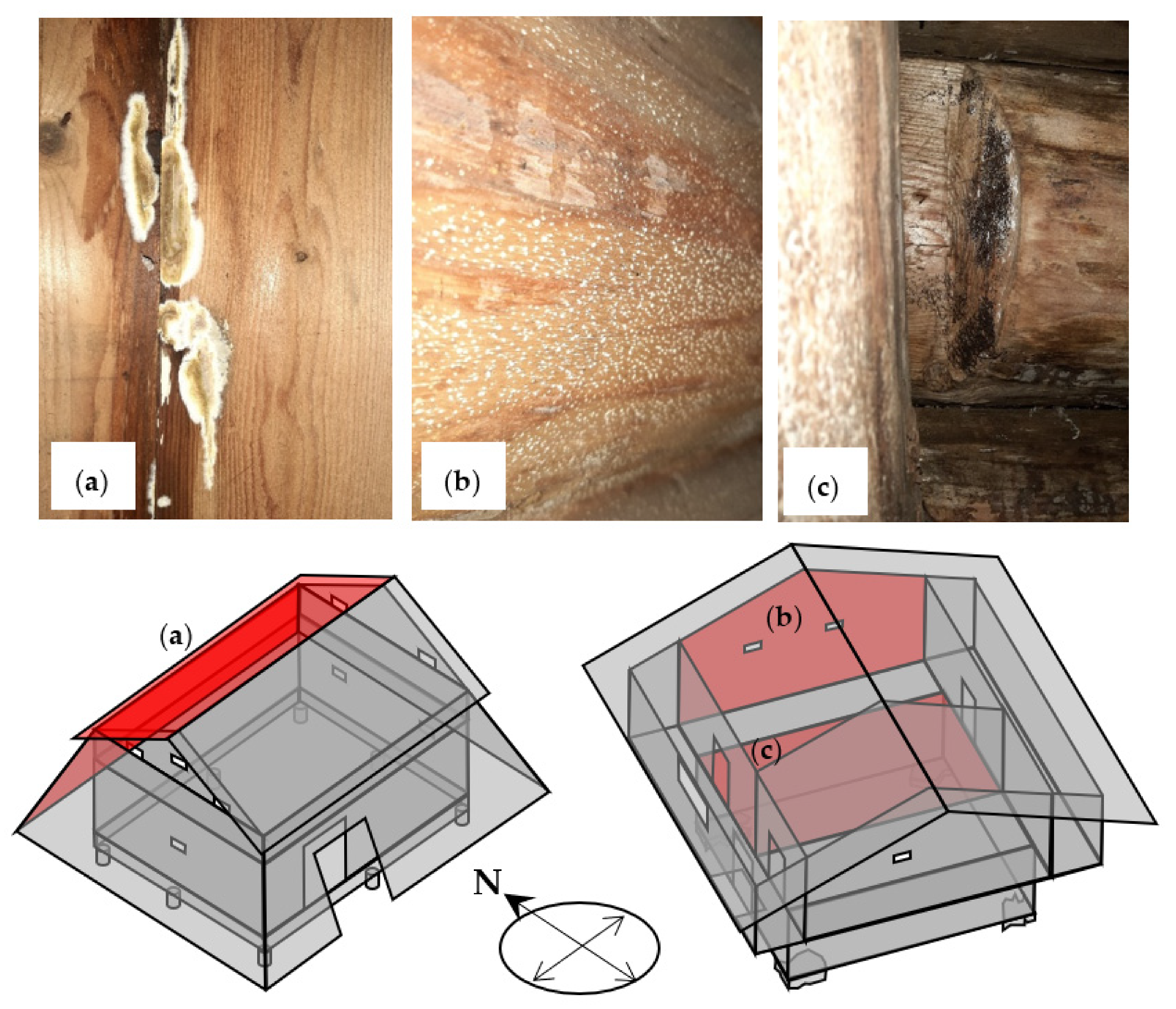
(a) Brown-rot fungi (Coniophora puteana) detected at the positions highlighted with red color at the Fadum storehouse. (b) Scopulariopsis colonies and (c) Myxomycetes detected at the positions highlighted with red color at the Heierstad loft.
Figure 7.
(a) Brown-rot fungi (Coniophora puteana) detected at the positions highlighted with red color at the Fadum storehouse. (b) Scopulariopsis colonies and (c) Myxomycetes detected at the positions highlighted with red color at the Heierstad loft.
Figure 8.
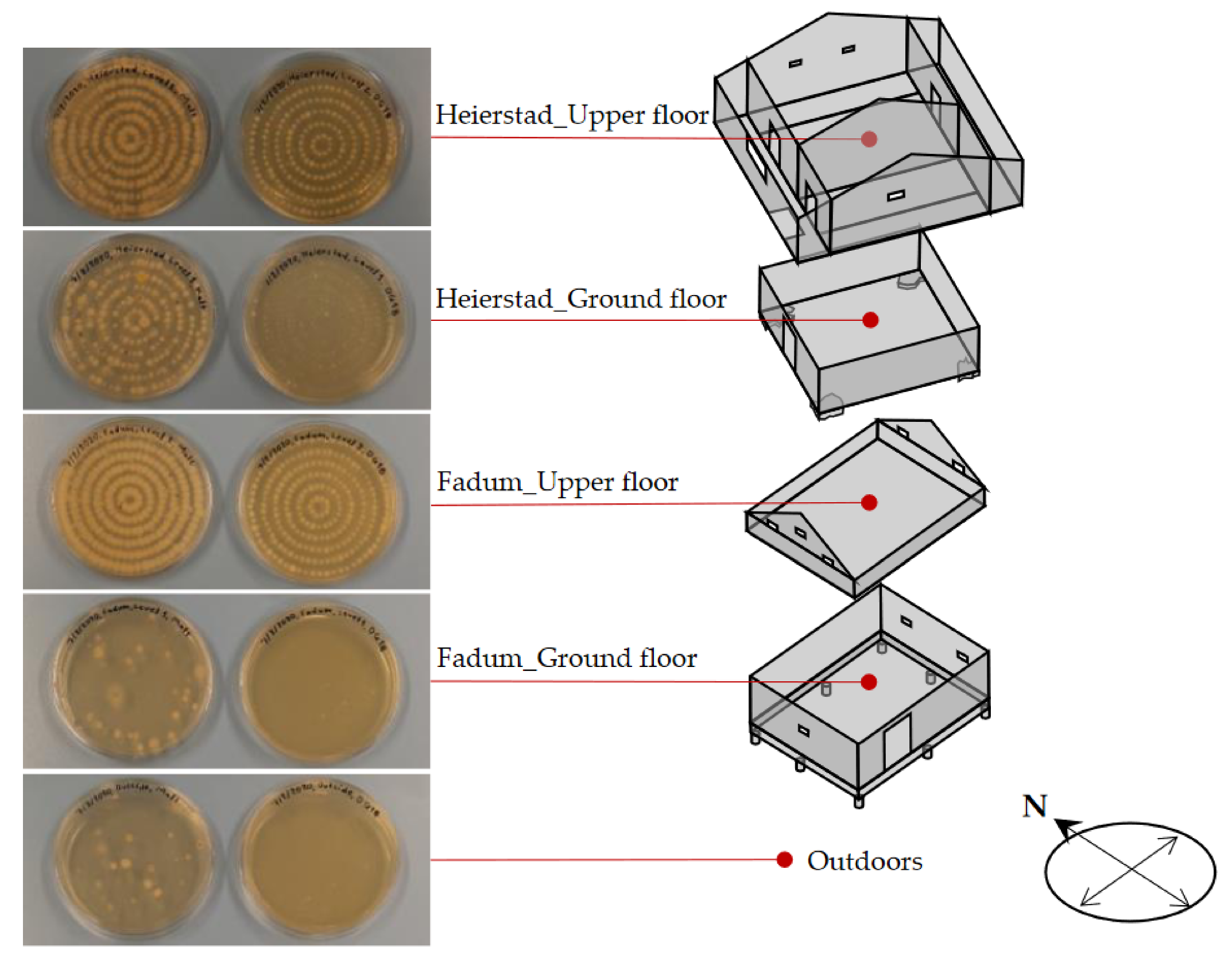
Positions of aerosol sampling and fungi colonies grown after 3 days at 25 °C on malt agar (plates on the left side of the pictures) and on DG-18 agar (plates on the right side of the pictures).
Figure 8.
Positions of aerosol sampling and fungi colonies grown after 3 days at 25 °C on malt agar (plates on the left side of the pictures) and on DG-18 agar (plates on the right side of the pictures).
Figure 9.
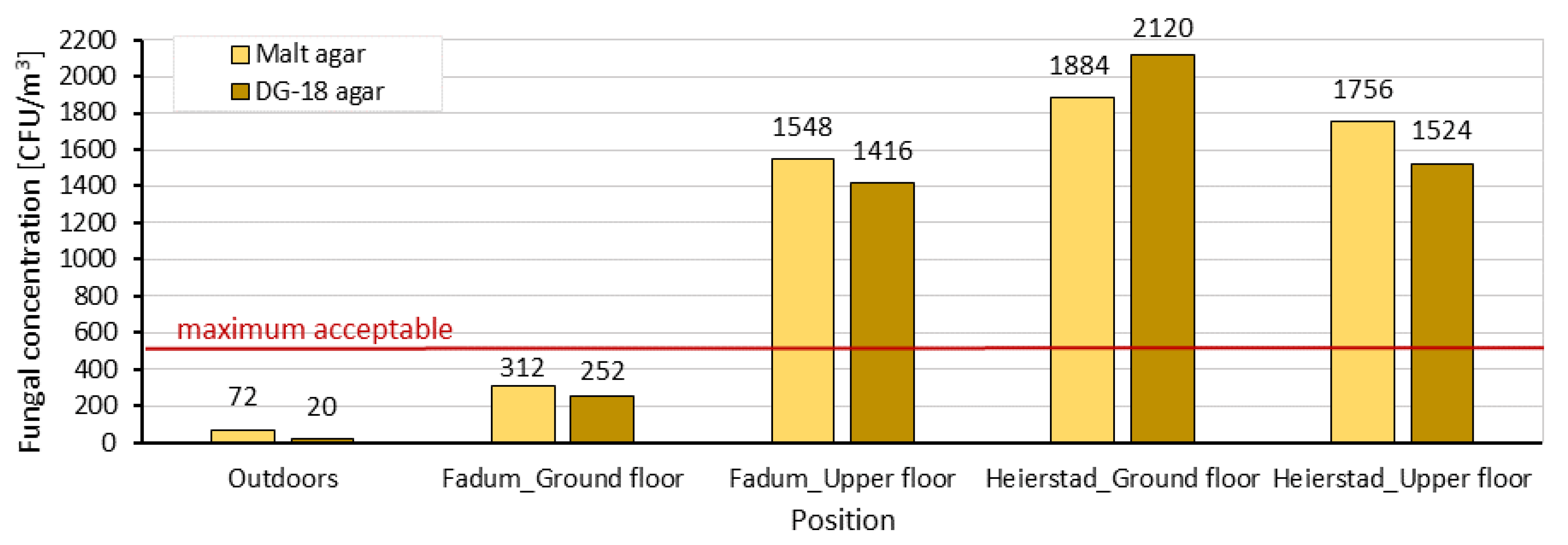
Fungal concentration in the two case studies considering the number of colony forming units found on the plates. The maximum acceptable value of 500 CFU/m
3 for noncontaminated indoor environments [
43] is highlighted with the red line.
Figure 9.
Fungal concentration in the two case studies considering the number of colony forming units found on the plates. The maximum acceptable value of 500 CFU/m
3 for noncontaminated indoor environments [
43] is highlighted with the red line.
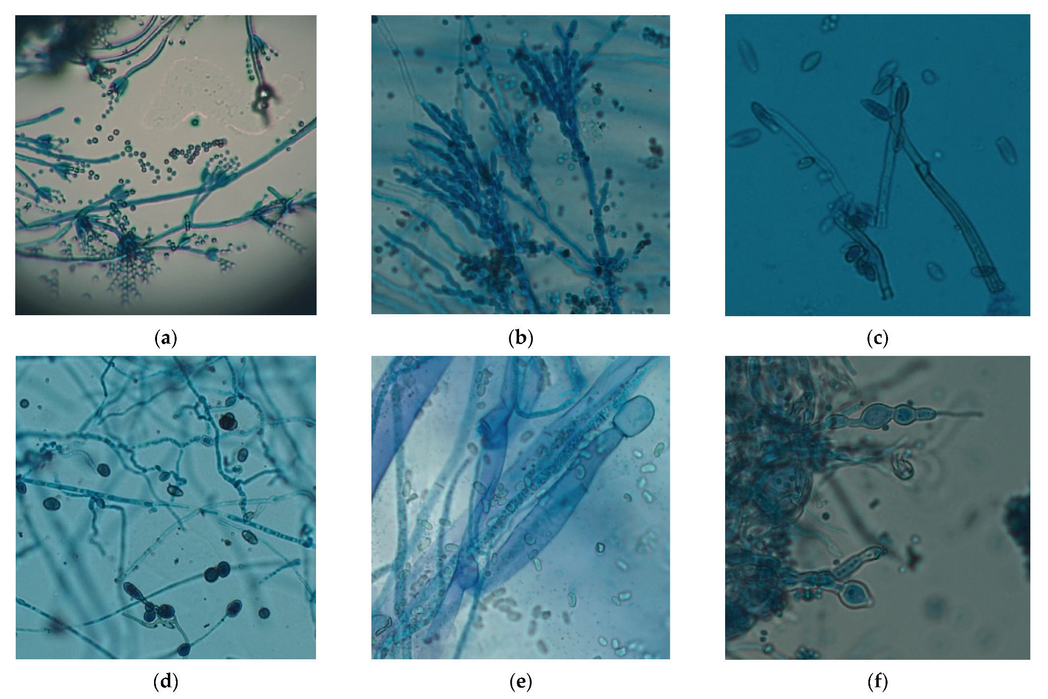
Figure 10.
Fungal structures of (a) Penicillium spp., (b) Aureobasidium spp., (c) Cladosporium spp., (d) Alternaria spp., (e) Mucor spp., and (f) Scopulariopsis spp. after methylene blue staining.
Figure 10.
Fungal structures of (a) Penicillium spp., (b) Aureobasidium spp., (c) Cladosporium spp., (d) Alternaria spp., (e) Mucor spp., and (f) Scopulariopsis spp. after methylene blue staining.
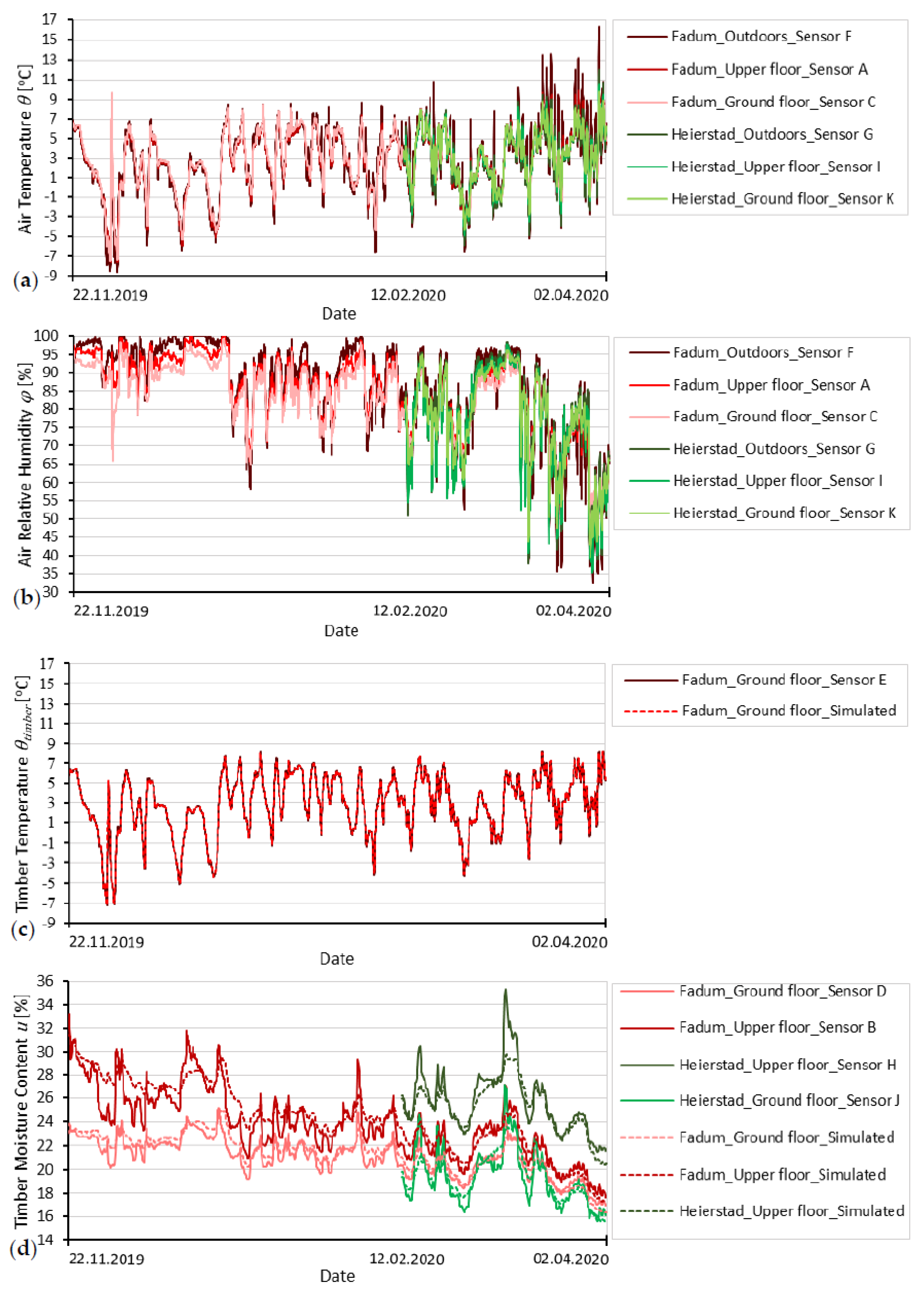
Figure 11.
Measurements of the (a) air temperature and (b) relative humidity, which have been used as boundary conditions in the hygrothermal models, and both measured and simulated (c) temperature and (d) moisture content in the timber building components.
Figure 11.
Measurements of the (a) air temperature and (b) relative humidity, which have been used as boundary conditions in the hygrothermal models, and both measured and simulated (c) temperature and (d) moisture content in the timber building components.
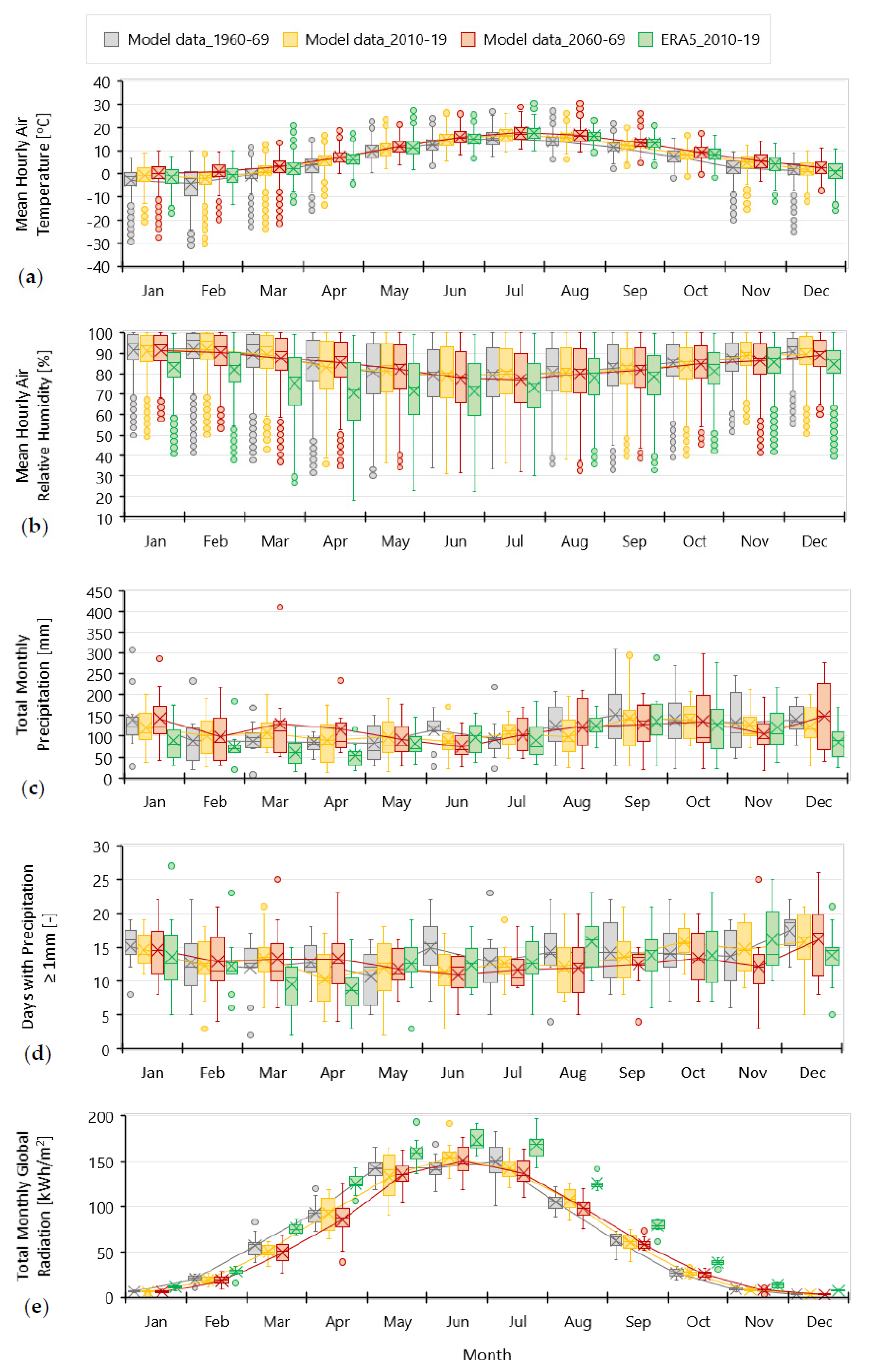
Figure 12.
Comparison among (a) air temperature, (b) air relative humidity, (c,d) precipitation and (e) radiation data derived from the MPI-ESM-LR_REMO2015 model and ERA5 reanalysis. In the boxplots the box shows 50% of the data, with median represented as a horizontal bar and the average value highlighted with the ‘x’ symbol. The whisker extends to two standard deviations of the data and the circles represent the outliers.
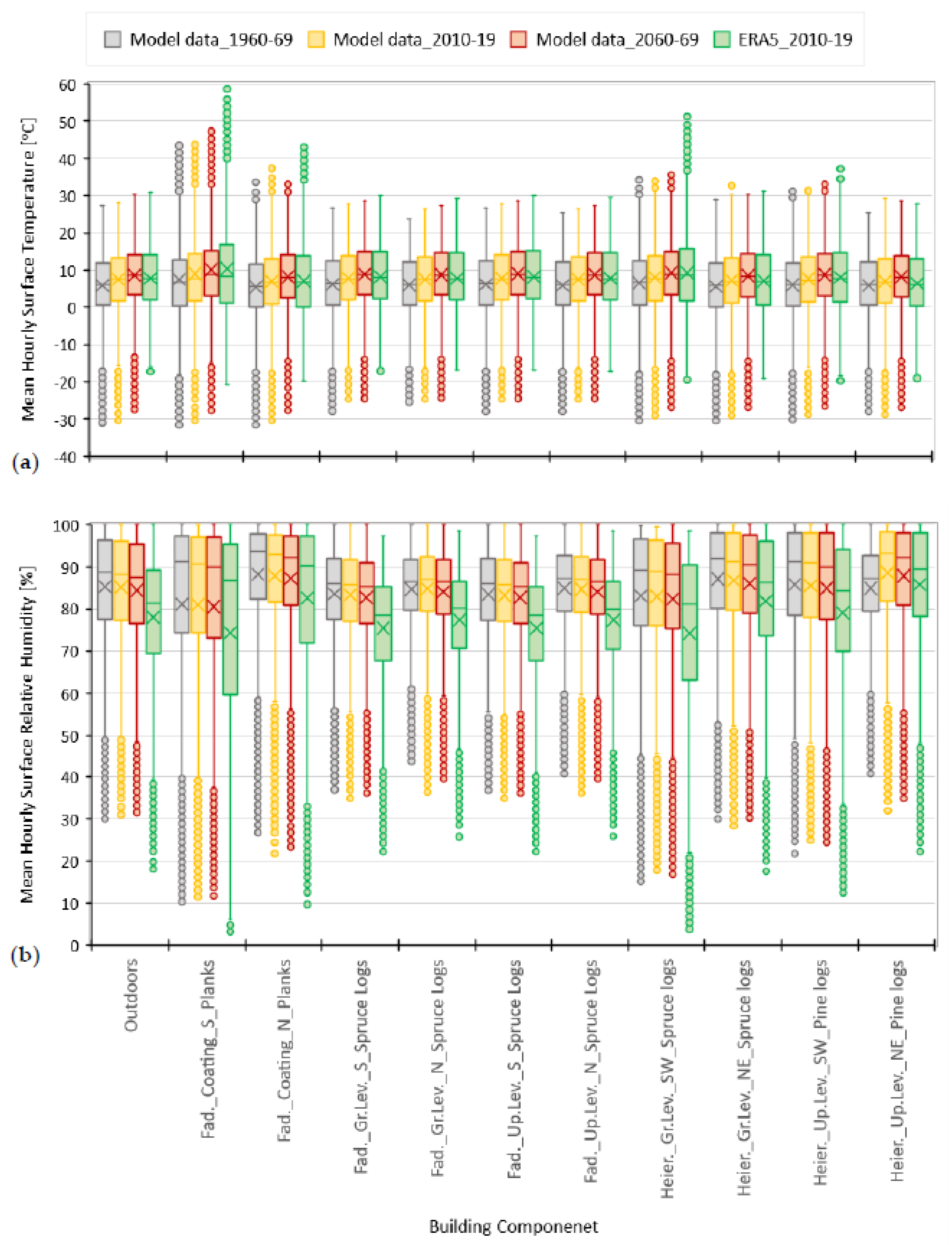
Figure 13.
Distribution of (a) hourly surface temperature and (b) hourly surface relative humidity for the exterior surface of selected building components. In the boxplots the box shows 50% of the data, with median represented as a horizontal bar and the average value highlighted with the ‘x’ symbol. The whisker extends to two standard deviations of the data, and the circles represent the outliers.
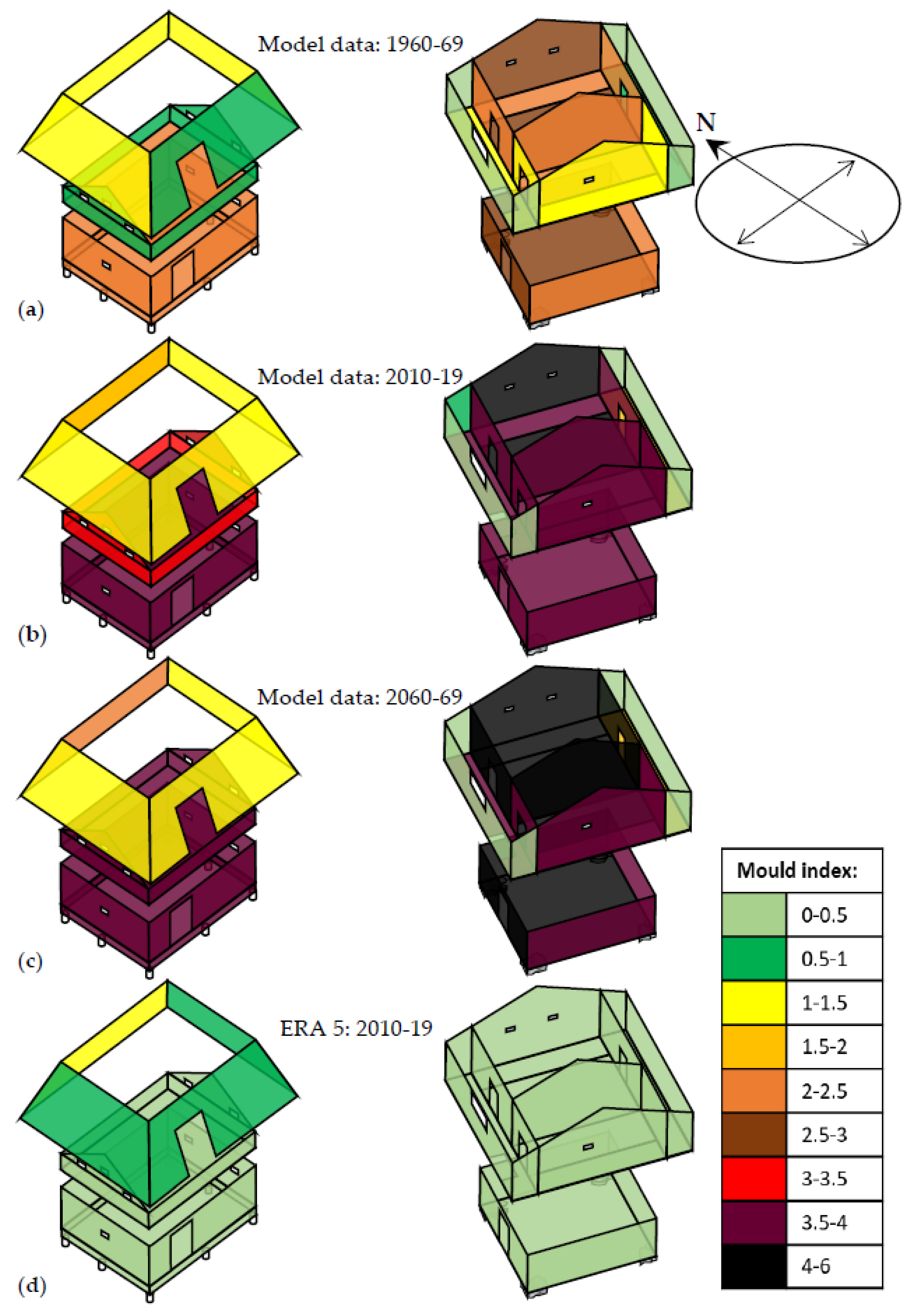
Figure 14.
Average values of annually maximum mold indices under (a) past, (b) current, and (d) future climate conditions, considering climate data from MPI-ESM-LR_REMO2015 model. (d) Respective results for the current conditions by considering climate data from the ERA5 reanalysis. The results refer to the interior surfaces of the building components, with the exception of the coating of the Fadum storehouse where the exterior side is taken into account.
Table 1.
Inputs, outputs, and origin of the measurements to validate the outputs of the simulated hygrothermal performance of selected building components.
Table 1.
Inputs, outputs, and origin of the measurements to validate the outputs of the simulated hygrothermal performance of selected building components.
| Group | 1D Hygrothermal Simulations | Origin of Measurements to Validate the Output |
|---|
| Component | Input Climate | Output |
|---|
| Interior θ, φ | Exterior θ, φ |
|---|
| II | Log at the southern wall of the ground level of the Fadum storehouse | Sensor C | Sensor F | θtimber 1 | Sensor E |
| u 1 | Sensor D |
| Log at the southern wall of the upper level of the Fadum storehouse | Sensor A | Sensor F | u 1 | Sensor B |
| III | Log at the northwest wall of the ground level of the Heierstad loft | Sensor K | Sensor G | u 1 | Sensor J |
| IV | Log at the northwest wall of the upper level of the Heierstad loft | Sensor I | Sensor G | u 1 | Sensor H |
Table 2.
Description of the mold growth index [
41].
Table 2.
Description of the mold growth index [
41].
| Index | Growth Rate | Description |
|---|
| 0 | No growth | Spores not activated |
| 1 | Small amounts of mold on surface (microscope) | Initial stages of growth |
| 2 | <10% coverage of mold on surface (microscope) | - |
| 3 | 10–30% coverage of mold on surface (visual) | New spores produced |
| 4 | 30–70% coverage of mold on surface (visual) | Moderate growth |
| 5 | >70% coverage of mold on surface (visual) | Plenty of growth |
| 6 | Very heavy and tight growth | Coverage around 100% |
Table 3.
Parametrization of the updated VTT mold model based on the features of the examined surfaces.
Table 3.
Parametrization of the updated VTT mold model based on the features of the examined surfaces.
| Surface Description | W | SQ | k1 | k2 (Mmax) | Cmat |
|---|
| M < 1 | M ≥ 1 | A | B | C | φmin [%] |
|---|
| Log/plank treated with tar | 0 | 0 | 0.072 | 0.097 | 0.0 | 5 | 1.5 | 85 | 1 |
| Log without treatment | 0 | 0 | 1.000 | 2.000 | 1.0 | 7 | 2.0 | 80 | 1 |
| Plank without treatment | 0 | 0 | 0.578 | 0.386 | 0.3 | 6 | 1.0 | 80 | 1 |
| Degraded surface (positions with cracks, splits, etc.) | 0 | 1 | 1.000 | 2.000 | 1.0 | 7 | 2.0 | 80 | 1 |
Table 4.
Fungi genera identified from the samples collected from the two case studies.
Table 4.
Fungi genera identified from the samples collected from the two case studies.
| Fungi Genera | Fadum Storehouse | Heierstad Loft |
|---|
| Penicillium spp. | ✓ | ✓ |
| Aureobasidium spp. | ✓ | ✓ |
| Cladosporium spp. | ✓ | ✓ |
| Alternaria spp. | ✓ | ✓ |
| Scopulariopsis spp. | ✓ | ✓ |
| Mucor spp. | ✓ | |
Table 5.
Selection of material properties for the logs of the two case studies by examining the goodness of fit between measured and simulated hygrothermal performance.
Table 5.
Selection of material properties for the logs of the two case studies by examining the goodness of fit between measured and simulated hygrothermal performance.
| Group | Group Description | Test Component | Test Parameter | Goodness of Fit |
|---|
| a 1 | b 1 | c 1 | d 1 | e 1 |
|---|
| II | Logs forming the walls and floors of the Fadum storehouse | Log at the southern wall of the ground level | θtimber | 92.9 | 92.9 | 93.5 | 94.1 | 90.2 |
| u | 44.5 | 31.1 | 57.4 | 24.5 | 1.74 |
| Log at the southern wall of the upper level | u | 56.9 | 17.7 | 57.2 | 38.7 | 4.3 |
| III | Logs forming the walls and floors of the ground level of the Heierstad loft | Log at the northwest wall of the ground level | u | 28.3 | 20.7 | 43.0 | 44.2 | 7.7 |
| IV | Logs forming the walls and floors of the upper level of the Heierstad loft | Log at the northwest wall of the upper level | u | 7.2 | 0.3 | 8.29 | 13.2 | 48.3 |
Table 6.
Average values of annually maximum mold indices by taking into account all different substrate surfaces of the case studies, the atmospheric temperature, and the relative humidity under four different climatic excitations.
Table 6.
Average values of annually maximum mold indices by taking into account all different substrate surfaces of the case studies, the atmospheric temperature, and the relative humidity under four different climatic excitations.
| Surface Description | Climate Model Data | ERA5 |
|---|
| 1960–69 | 2010–19 | 2060–69 | 2010–19 |
|---|
| Log/plank treated with tar | 0.0 | 0.0 | 0.0 | 0.0 |
| Log without treatment | 5.7 | 5.7 | 5.8 | 1.1 |
| Plank without treatment | 1.1 | 1.3 | 1.5 | 0.2 |
| Degraded surface (positions with cracks) | 5.8 | 5.8 | 5.9 | 4.5 |


